Assessment of Water Quality in Lake Qaroun Using Ground-Based Remote Sensing Data and Artificial Neural Networks

Abstract

Monitoring and managing water quality parameters (WQPs) in water bodies (e.g., lakes) on a large scale using sampling-point techniques is tedious, laborious, and not highly representative. Hyperspectral and data-driven technology have provided a potentially valuable tool for the precise measurement of WQPs. Therefore, the objective of this work was to integrate WQPs, derived spectral reflectance indices (published spectral reflectance indices (PSRIs)), newly two-band spectral reflectance indices (NSRIs-2b) and newly three-band spectral indices (NSRIs-3b), and artificial neural networks (ANNs) for estimating WQPs in Lake Qaroun. Shipboard cruises were conducted to collect surface water samples at 16 different sites throughout Lake Qaroun throughout a two-year study (2018 and 2019). Different WQPs, such as total nitrogen (TN), ammonium (NH₄⁺), orthophosphate (PO₄³⁻), and chemical oxygen demand (COD), were evaluated for aquatic use. The results showed that the highest determination coefficients were recorded with the NSRIs-3b, followed by the NSRIs-2b, and then followed by the PSRIs, which produced lower R² with all tested WQPs. The majority of NSRIs-3bs demonstrated strong significant relationships with three WQPs (TN, NH₄⁺, and PO₄³⁻) with (R² = 0.70 to 0.77), and a moderate relationship with COD (R² = 0.52 to 0.64). The SRIs integrated with ANNs would be an efficient tool for estimating the investigated four WQPs in both calibration and validation datasets with acceptable accuracy. For examples, the five features of the SRIs involved in this model are of great significance for predicting TN. Its outputs showed high R² values of 0.92 and 0.84 for calibration and validation, respectively. The ANN-PO₄³⁻VI-17 was the highest accuracy model for predicting PO₄³⁻ with R² = 0.98 and 0.89 for calibration and validation, respectively. In conclusion, this research study demonstrated that NSRIs-3b, alongside a combined approach of ANNs models and SRIs, would be an effective tool for assessing WQPs of Lake Qaroun.

1. Introduction

The quality of surface water is a critical worldwide environmental concern, since it is essential for long-term economic progress and environmental protection. The status of water quality is based on several physicochemical parameters [1]. Therefore, WQPs are essentially concerned with carefully constructed water quality metrics that are difficult to effectively interpret, since the condition of water quality status is dependent on several physiochemical properties [2,3]. Furthermore, the typically huge amounts of water quality data provided by monitoring systems sometimes creates difficulties for water managers in performing effective evaluations [4]. Contamination of surface water resources has become a serious environmental issue on a worldwide scale, requiring regular assessment and observation throughout all altitudes for ecosystem sustainability [5,6,7].

According to the US Environmental Protection Agency’s (USEPA) [8] most current national water quality surveys, more than a third of our lakes, as well as nearly half of our rivers and streams, are polluted. According to the United Nations (UNEP) [9], over 80% of the world’s wastewater is dumped into the environment without being cleaned or repurposed. In certain developing nations, the ratio is as high as 95%. On average, most cities in developing countries generate 30–70 mm³ of wastewater per person every year [10].

Shallow lakes are necessary ecological and socio-economic resources worldwide. However, human activities have caused deterioration for the ecological status of sallow lakes in many regions of the world. Thus, there is a crucial interest in the precise evaluation and careful monitoring of ecological status in shallow lakes [11]. Multiple contamination sources are observed along the lake’s southern shore, comprising agricultural and industrial wastewater flows from the El-Fayoum region, as well as fisheries [12,13,14].

The term WQPs refers to the identification of various chemical, physical, and biological properties of water bodies, as well as determining the possible pollution sources that lead to the deterioration of water quality in these bodies [15]. The WQPs should be monitored and assessed, not just to evaluate the influence of different pollutants, but also to conserve aquatic life and follow efficient water management strategies [16]. Water quality status can be evaluated for aquatic environment using several parameters, such as total dissolved solids (TDS), temperature (T °C), hydrogen ion concentration (pH),total nitrogen (TN), ammonium (NH₄⁺), orthophosphate (PO₄³⁻), and chemical oxygen demand (COD). The physicochemical characteristics of surface water are considered significant parameters of contamination in aquatic environments. For example, major nutritional components such as TN, NH₄⁺, and PO₄³⁻ also play a vital role in aquatic environmental quality by maintaining the food chain of phytoplankton, zooplankton, and fish [17]. Nutritional constituents have always been considered as an indicator of the prospective fertility of water sources, reflecting both natural processes and human activities and their influence on the quality of lake water [18]. Furthermore, COD is commonly utilized to determine industrial, domestic, and agricultural waste contents, and the quantity of abiotic oxidizable substances in water, as well as the levels of total oxygen consumption in water [19].

Analytical analyses employed to determine and assess water quality characteristics are costly, complex, and time consuming. The monitoring data of the contaminant indicates the types of contaminants and their trends in an aquatic ecosystem, allowing water quality regulators to provide suggestions for future forecasting [20,21]. New approaches and procedures for monitoring water quality are being developed as technology advances and its functions are extended. Water quality may be investigated utilizing cutting-edge methods such as geospatial (GIS) spectral analysis of water, and statistical modeling to save money and time while increasing accuracy [22]. In this regard, the efficient resolving and panoramic data obtained by various remote sensing platforms and GIS may be a robust tool in the construction of highly effective strategies for assessing and monitoring ecological status in shallow lakes system, and also provide insights into the functions of various ecosystems, showing how they respond to environmental changes [21].

Remote sensing or ground-based remote sensing technologies can offer a sensible significant contribution to the monitoring of shallow lakes, since they may be able to provide quantitative large-scale panoramas of water quality status in shallow lakes [23]. The properties of spectral reflectance of the water surface at different wavebands along the electromagnetic spectrum can be used as indicators for the change in chemical and physical constituents of water [24,25]. t Many previous studies revealed that many WQPs, such as TN, chlorophyll concentration, turbidity, total dissolved solids (TDS), and PO₄³⁻, can be estimated via remotely sensed data [26,27,28,29,30]. Therefore, remotely sensed data would be an effective tool for decision makers to assess water-bodies more efficiently. To enhance the efficiency of remotely sensed data for monitoring and assessing lake systems, efforts are vital to determine the optimum algorithm formulations for estimating different WQPs [31]. Therefore, it may be useful to further demonstrate the efficacy of various methods to the formulation of remotely sensed based algorithms for the quantification of WQPs of shallow lakes. In this study, the optimized newly two- and three-band of spectral reflectance indices (SRIs) were calculated from two- and three-dimensional slice maps.

The prediction of WQPs in shallow lakes is a serious issue in maintaining the ecosystem at a safe level. In this regard varying deterministic models have been employed in the past decades [32]. However, practically, the statistical efficiency of different deterministic models is normally weak, since actual natural ecosystems tend to be too complex for these state-of-the-art models. Artificial Neural Networks (ANNs) may provide a fast and reliable technique for creating models for the estimation of different WQPs in lake systems. ANNs are able to generalize non-linear patterns within a dataset, and can solve complicated problems [33]. Methods based on machine learning, such as ANNs, are increasingly being applied to solve environmental challenges. These data-driven strategies can be used to solve problems that are extremely nonlinear [34]. ANNs have been successfully applied to assess the accuracy of water quality constituent prediction [35].

There is a scarcity of data on the effectiveness of ANNs models integrated with SRIs for estimating WQPs (TN, NH4⁺, PO4³⁻, and COD). The major purpose of this research was to develop effective tools for making informed judgments about Lake Qaroun’s water quality in order to ensure efficient management, identify pollution sources, and provide a clear picture of how sampling strategies should be redesigned. This research study was based on the hypothesis that ground-based remotely sensed data and machine learning modeling would be effective tools for assessing WQPs in Lake Qaroun.

Therefore, the specific objectives of this research study were to: (i) assess the water quality status of Lake Qaroun using four WQPs (TN, NH₄⁺, PO₄³⁻, and COD) integrated with geospatial techniques; (ii) build the two- and three-dimensional slice map based on spectral bands to detect the optimized NSRIs-2b and NSRIs-3b; (iii) evaluate the accuracy of three different groups of SRIs (PSRIs, NSRIs-2b, and NSRIs-3b) in quantifying WQPs; and (iv) evaluate the performance of ANNs models linked with SRIs in quantifying the WQPs.

2. Materials and Methods

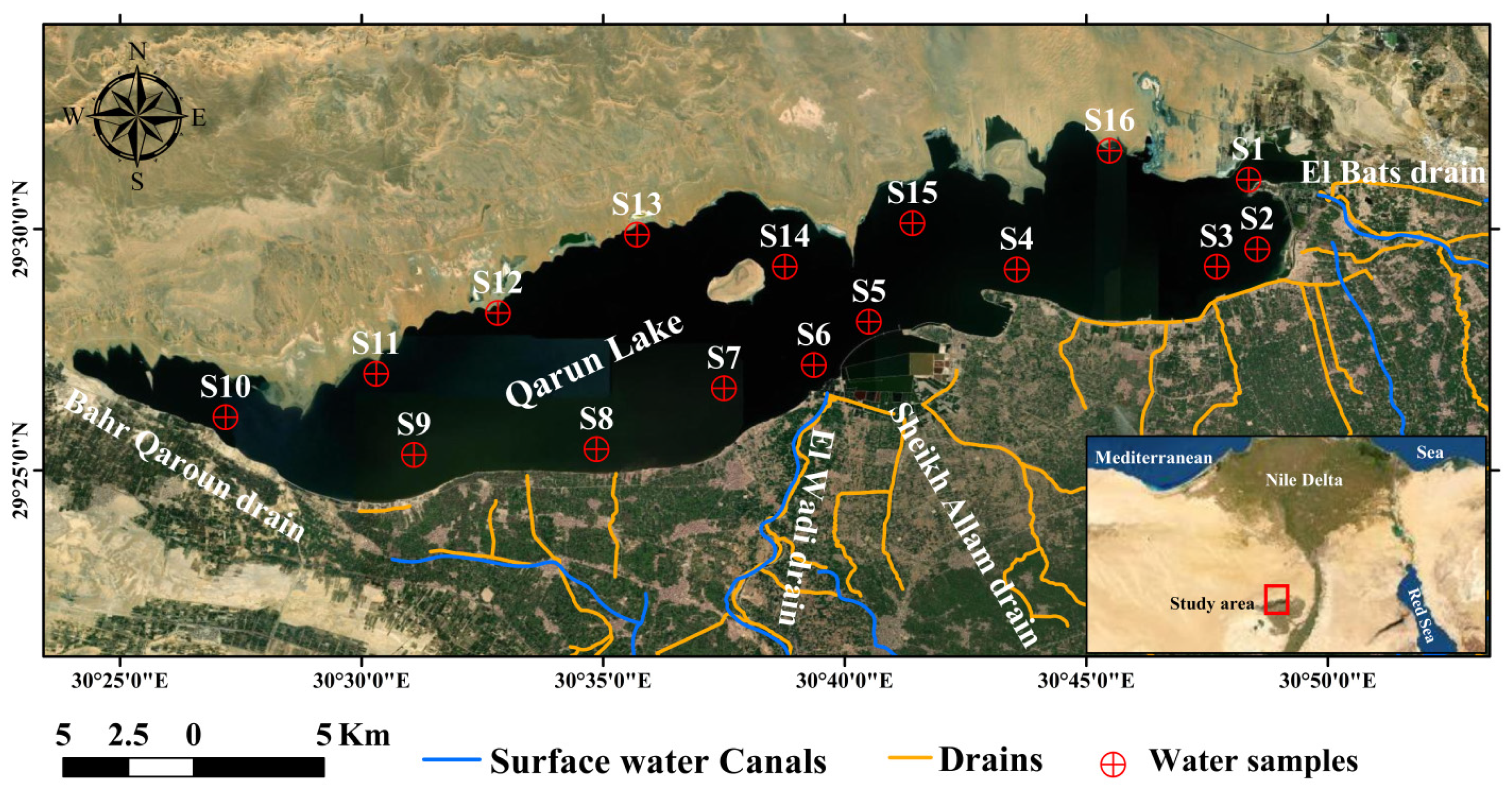
2.1. Study Site and Description

Lake Qaroun is an important inland aquatic environment with a total area of approximately 200 km², located in Egypt’s Western Desert, between the latitudes of 29°24′ and 29°33′ N and longitudes of 30°24′ and 30°50′ E (Figure 1). The lake’s peripheries have water depths ranging from 2 to 5 m, while the central area has an 8 m depth [36]. The minimum and maximum values of annual mean temperatures, rainfall, and evaporation rate are 14.5 °C and 31.0 °C, 0.6 mm and 4 mm, and 1.9 mm/day and 7.3 mm/day, respectively [37]. The research area is more or less rectangular and elongated in design, measuring an average of 45 km long, 5.7 km wide, and 4.2 m deep, acting as a natural discharge zone for the El-Fayoum area [17]. Furthermore, the lake is significant for fishing, salt manufacturing, tourism, and migrating birds [38]. Therefore, Lake Qaroun has been classified as a natural restricted area, although it has recently been safeguarded from various contaminating factors [12,36,39]. It is well known that contamination of surface water by inorganic and organic compounds is a severe danger to aquatic ecosystems, as a result of increasing industrialization and urbanization [12,17,36]. The lake is mainly encompassed by urban and agricultural regions to the south and east, and by uninhabited desert lands to the north and west. Lake Qaroun acts as a large natural reservoir for varying wastes (agricultural, domestic, sewage, and industrial wastes) coming from a large area of El Fayoum Province that flows through the eastern and southern drains (El-Bats, El-Wadi, Sheikh Allam, and Bahr Qaroun), as well as a number of narrower drains that go into the lake [40]. The research site is a confined shallow brackish lake with no discharge exits.

2.2. Sampling and Analyses

Over the course of a two-year investigation, water samples were gathered (2018 and 2019). Water samples were collected from 16 sites to cover the whole lake (Figure 1). Using a hand-held GPS device (MAGELLAN GPS 315, U.S.), each sampling location was pinpointed, with an accuracy of approximately 7 m in both vertical and horizontal directions. The accuracy of determining locations was maintained by repeatedly identifying the location of fixed points with respect to the sources of pollution. Sampling locations were selected carefully across Lake Qaroun in order to have a good representation of the spatial variability of WQPs throughout the entire lake. A mobile calibrated glass electrode multi-parameter (YSI Professional Plus, Portugal) was used to determine several physicochemical parameters, including TDS, pH, and temperature in water samples, with an accuracy of approximately 10 mg/L, 0.02 and 0.2 °C, respectively. Water samples were collected in polyethylene bottles, labeled, kept in an ice box, and were taken to the laboratory for various analyses within 48 h. Total nitrogen (TN) was measured in unfiltered water samples in the lab using the 2,6-dimethylphenol procedure after persulfate digestion. A UV/Visible multiparameter bench photometer (HI 81226, Romania) was used to determine the concentration of NH₄⁺, PO₄³⁻, and COD, with an accuracy of approximately 0.01 mg/L, 0.01 mg/L, and 1 mg/L, respectively. Water sample tests were carried out using established techniques for water-wastewater analysis. To enhance data confidence of the analytical technique, duplicates of samples were conducted during quality assurance and quality control (QA/QC) analysis. Authenticated reference materials were used to ensure procedural accuracy (ERM-CA713).

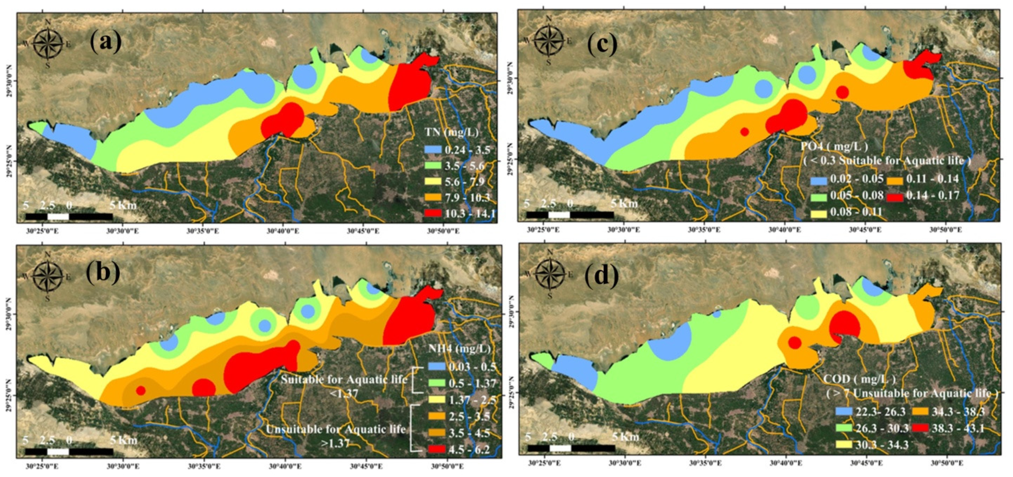
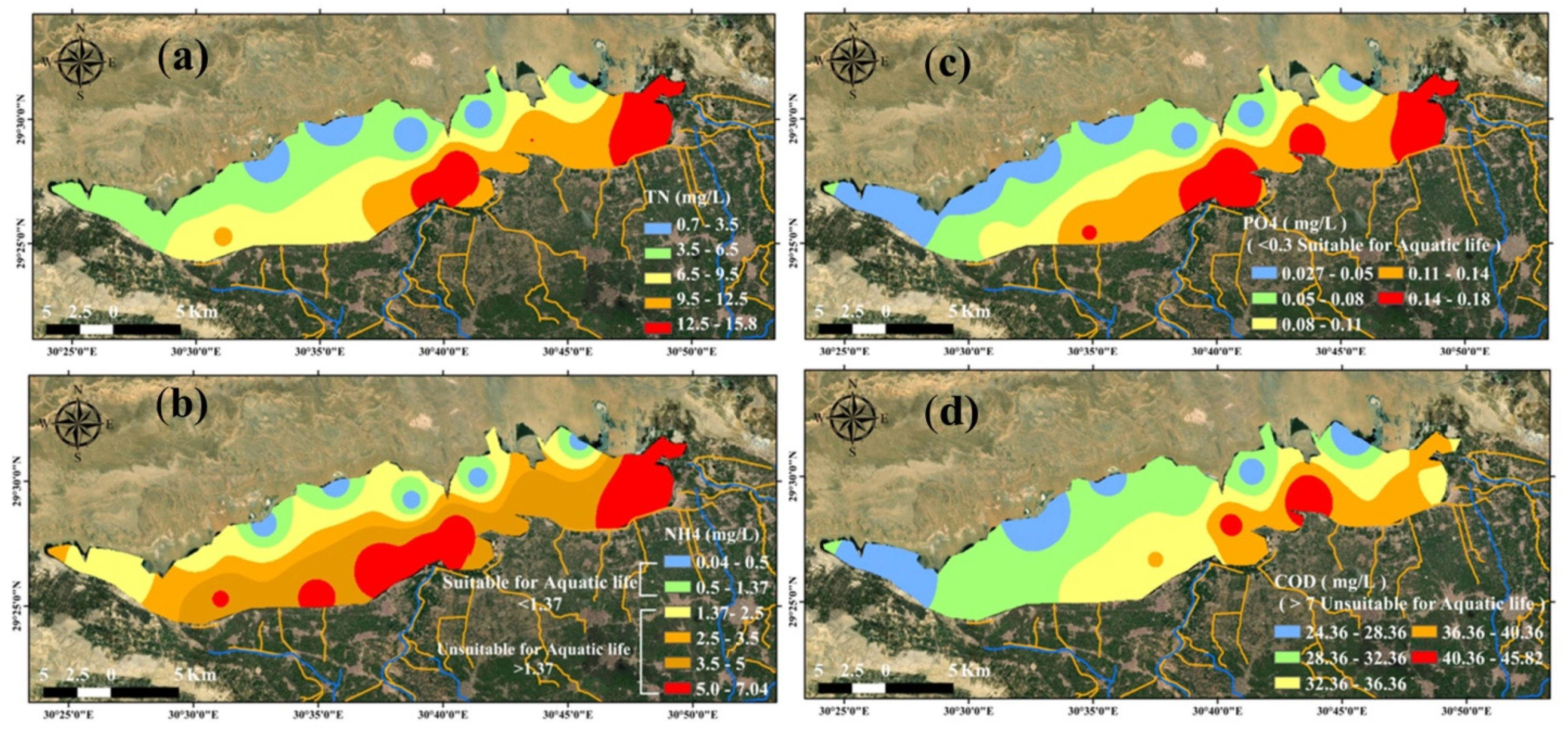
2.3. Spatial Distributions of WQPs

The ArcGIS Spatial Analyst package v.10.2.1 has various tools for analysis of spatial data that utilize statistical theory, and methodologies to model spatially referenced data. The interpolation methods in ArcGIS Spatial Analysis were utilized to identify the intervening values for the four tested WQPs. GIS was used to establish the maps of different tested WQPs through the inverse distance weighted interpolation (IDW) procedure, which is well famed as one of the simplest and most commonly used interpolation procedures to map varying water quality parameters. Using the records at certain stations, the results can be extrapolated to determine the value at non-sampled locations [41,42,43,44]. An efficient method to specify the most suitable interpolation method or the studied parameters is the calculation of the root mean square error (RMSE) by running an aggregate error analysis on the interpolation, following across the validation routine. It can be performed by removing one data point at a time, and it estimates the value using the interpolation method and all other data points. This method generates a residual error at each data point location (residual error = measured data value at the point—estimated value). This technique was applied on all collected samples. The RMSE was calculated from the collection of residual errors.

2.4. Spectral Reflectance Measurements

The spectral measurements of the above- surface radiance were made at each sampling point across Lake Qaroun using a handheld spectrometer, according to Elsayed [30,45]. The instrument has a spectral band which ranged from 302 to 1148 nm. The measurements of the reflectance from water surfaces was restricted between 11:00 and 13:00 p.m. in order to minimize the effect of solar zenith changes. The detector was adjusted at nadir position at approximately 0.25 m above the water surface at all sampling sites, with a 0.05 m² scanning area. A calibration factor derived from a white reference standard was used to correct the reflectance data. Each water sample’s spectral reflectance was repeated three times, and then the mean spectrum was calculated. Lastly, the obtained spectra were smoothed to reduce the electromagnetic spectrum’s noise.

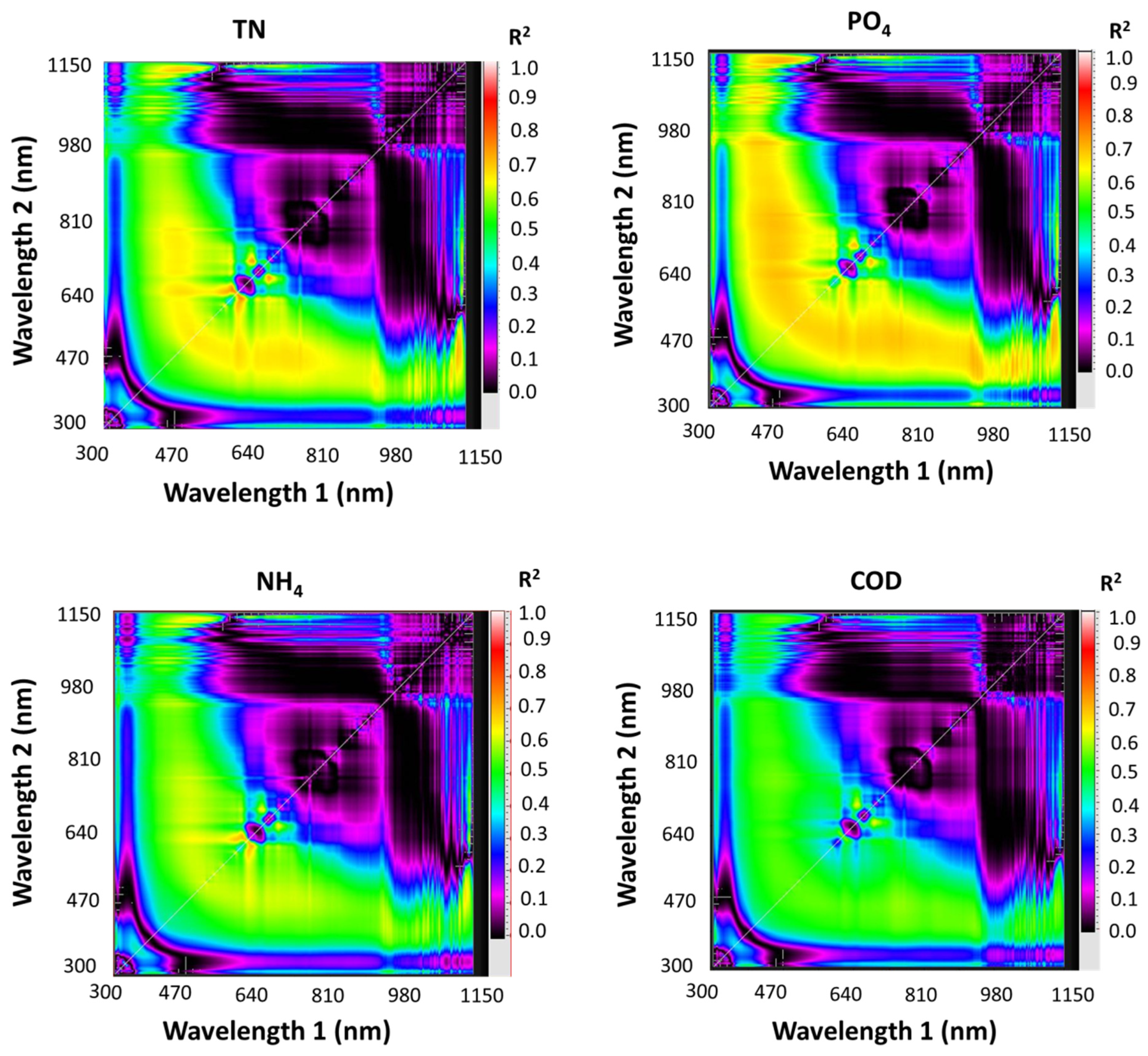
2.5. Selection of Published, Newly Two and Three Band SRIs

Five commonly band-ratio and band combinations used indices, and 13 newly extracted SRIs were chosen in this study for the estimation of four WQPs (Table 1). To identify the best combination of two-band (2-D) and three-band (3-D) SRIs for identifying WQPs, all possible combinations of bands ranging from 302 nm to 1148 nm were calculated based on correlation matrices [30], which were established using the pooled data of both investigated years for each water quality indicator (n = 32). The 2D and 3D slice maps of determination coefficient (R²) values were constructed, which showed sequential linear regression between different spectral indices and various WQPs. The SRIs with the highest R² were selected.

The two-band ratio SRIs were calculated as a ratio spectral index (RSI) from all potential two-band ratio combinations covering the wavelengths from 302 nm to 1148 nm, according to the following equation:

RSI = R₁/R₂

(1)

where R₁ and R₂ are the spectral reflectance values at wavelengths ranging from 302 nm to 1148 nm.

3-D slice maps of R² that were determined for the relationship between different WQPs and the normalized spectral index (NSI) that was quantified to the greatest extent possible combination of three bands over spectral bands from 390 to 750 nm were based on the following equation:

NSI = (R₁ − R₂ − R₃)/(R₁ + R₂ + R₃)

(2)

where R₁, R₂, and R₃ are the spectral reflectance values at wavelengths ranging from 390 nm to 750 nm.

The lattice package in R statistics v. 3.0.2 (R Foundation for Statistical Computing, 2013) was used to extract different 2-D correlogram maps, while MATLAB 7.0 (The MathWorks, Inc., Natick, MA, USA) was used to derive 3-D slice maps.

2.6. Artificial Neural Networks Technique

2.6.1. Back-Propagation Neural Network (BPNN)

The backpropagation neural network (BPNN) model is among the most predominantly used artificial neural networks [46]. The BPNN is mainly constructed based on three layers: (1) the input layer is basically a primitive dataset for the neural network; (2) the unseen layer is a medium layer between both independent variables and dependent output layers; and (3) the output layer ends up with the results of the specified inputs. The ANN is a type of machine learning mathematical technique that employs multiple layers to obtain high-advanced features from basic input data. Input layers are noted as vector I. The network has one hidden layer, and the number of nodes is estimated according to regression precision. The concealed layers symbolize the “activation” nodes, and are usually seen as weight. The final circle symbolizes the output layer that demonstrates the predicted value of a measured parameter. The model’s hyperparameters were the number of neurons in two hidden layers (1 to 25), and different activation functions (identity, logistic, tanh, and ReLu). A learning rule is a mathematical logic or technique that increases the performance and training time of an artificial neural network [22]. This rule is usually applied repeatedly across the network. The network was tried for at least 1500 iterations, or until the error measurement reached (10⁻⁴). To select the number of neurons in the unseen layer for this model, the cross-validation manner with the leave-one-out validation (LOOV) method was run on the training data set. The parameter of limited memory Broyden–Fletcher–Goldfarb–Shanno (lbfgs) was employed as a weight optimizer to effectively apply the algorithm [47]. To enhance the predictive capacity of the regression model and diminish hyperspectral image dimensionality, the following equation was used to estimate the most informative feature [48]:

$$M=\frac{{\sum }_{j=1}^{n_H}\left[\left({\left|I\right|}_{P_j}/{\sum }_{k=1}^{n_p}{\left|I\right|}_{{\mathrm{P}}_{j,k}}\right){\left|O\right|}_j\right]}{{\sum }_{i=1}^{n_p}\left({\sum }_{j=1}^{n_H}\left[\left({\left|I\right|}_{P_{i,j}}/{\sum }_{k=1}^{n_p}{\left|I\right|}_{P_{i,j,k}}\right){\left|O\right|}_j\right]\right)}$$

(3)

where M refers to the necessary parameter for the input variable, $n_p$ refers to the number of input variables, $n_H$ is the number of unseen layer nodes, ${\left|I\right|}_{P_j}$ represents the absolute value of the concealed layer rating corresponding to the pth input variable and the jth concealed layer, and ${\left|O\right|}_j$ refers to the absolute account of the output layer rating corresponding to the jth concealed layer.

The ANN model was optimized by selecting the best hyperparameters (number of neurons in two hidden layers, and activation function). Generally, the spectral indices of three SRIs groups were fed randomly to the model in the first loop, the low-level features were dropped during each loop, and the superb features were organized in an ascending order concerning the highest contribution. During looping, the best hyperparameters were adopted, and the rest were excluded. Subsequently, the ANN outputs were compared to identify high-ranking variants and superior hyperparameters at minimum RMSECV that could improve the prediction of WQP. More details about the CODs can be found in Table S1.

2.6.2. Model Evaluation

To assess the performance of a regression model, the following statistical parameters have been quantified: RMSE, and R² [49,50]. All parameters are explicated as follows: F_act is the real value that was estimated based on laboratory calculations, F_p is the predicted or simulated value, F_ave is the average value, and N is the total number of data points.

RMSE was calculated according to the following formula:

$$\mathrm{RMSE}=\sqrt{\frac{1}{N}{\sum }_{i=1}^N{\left(F_{ act}-F_{ p}\right)}^2}$$

(4)

Coefficient of determination:

$${\mathrm{R}}^2=\frac{\sum {\left(F_{ act}-F_{ p}\right)}^2}{\sum {\left(F_{ act}-F_{ ave}\right)}^2}$$

(5)

2.7. Data Analysis

The estimates of WQPs were subjected to statistical analysis to identify differences between the WQPs. Duncan’s test at a p value of ≤0.05 was run to compare the significant variations between the mean values of TN, NH₄⁺, PO₄³⁻, and COD, as well as different tested SRIs among 16 sampling points. A simple linear model was investigated to assess the relationships between the four assessed WQPs and varying types of SRIs across the two-year study. SPSS package (v. 12.0, SPSS Inc., Chicago, IL, USA) was used to perform the above statistical analysis of WQPs, and to calculate the values of WQPs (e.g., min, max, mean, and standard deviation).

Table 1. Description of the previously published and newly constructed spectral indices tested in this work.

SRIs	Formula	References
PSRIs
Ratio spectral index (RSI700,560)	R700/R560	[51]
Ratio spectral index (RSI700,675)	R700/R675	[52]
Normalized difference spectral index (NDSI699,705,670,677) (NDSI699,705,670,677)	(R699 − R705)/(R670 − R677)	[53]
Ratio spectral index (RSI833,1004)	R833/R1004	[54]
Normalized difference spectral index (NDSI560,520)	(R560 − R520)/(R560 − R520)	[55]
NSRIs-2b
Ratio spectral index
(RSI622,602)	R622/R602	This work
(RSI690,650)	R690/R650	This work
(RSI760,484)	R760/R484	This work
(RSI700,650)	R700/R650	This work
(RSI1130,500)	R1130/R500	This work
NSRIs-3b
Normalized difference spectral index
NDSI620,610,622	(R620 − R610 − R622)/(R620 + R610 + R622)	This work
NDSI700,650,712	(R700 − R650 − R712)/(R700 + R650 + R712)	This work
NDSI700,648,712	(R700 − R648 − R712)/(R700 + R648 + R712)	This work
NDSI648,712,696	(R648 − R712 − R696)/(R648 + R712 + R696)	This work
NDSI698,650,712	(R698 − R650 − R712)/(R698 + R650 + R712)	This work
NDSI620,614,602	(R620 − R614 − R602)/(R620 + R614 + R602)	This work
NDSI620,600,614	(R620 − R600 − R614)/(R620 + R600 + R614)	This work
NDSI696,710,652	(R696 − R710 − R652)/(R696 + R710 + R608)	This work

Table 1. Description of the previously published and newly constructed spectral indices tested in this work.

SRIs	Formula	References
PSRIs
Ratio spectral index (RSI700,560)	R700/R560	[51]
Ratio spectral index (RSI700,675)	R700/R675	[52]
Normalized difference spectral index (NDSI699,705,670,677) (NDSI699,705,670,677)	(R699 − R705)/(R670 − R677)	[53]
Ratio spectral index (RSI833,1004)	R833/R1004	[54]
Normalized difference spectral index (NDSI560,520)	(R560 − R520)/(R560 − R520)	[55]
NSRIs-2b
Ratio spectral index
(RSI622,602)	R622/R602	This work
(RSI690,650)	R690/R650	This work
(RSI760,484)	R760/R484	This work
(RSI700,650)	R700/R650	This work
(RSI1130,500)	R1130/R500	This work
NSRIs-3b
Normalized difference spectral index
NDSI620,610,622	(R620 − R610 − R622)/(R620 + R610 + R622)	This work
NDSI700,650,712	(R700 − R650 − R712)/(R700 + R650 + R712)	This work
NDSI700,648,712	(R700 − R648 − R712)/(R700 + R648 + R712)	This work
NDSI648,712,696	(R648 − R712 − R696)/(R648 + R712 + R696)	This work
NDSI698,650,712	(R698 − R650 − R712)/(R698 + R650 + R712)	This work
NDSI620,614,602	(R620 − R614 − R602)/(R620 + R614 + R602)	This work
NDSI620,600,614	(R620 − R600 − R614)/(R620 + R600 + R614)	This work
NDSI696,710,652	(R696 − R710 − R652)/(R696 + R710 + R608)	This work

3. Results and Discussion

3.1. Water Quality Parameters

During a two-year investigation, the WQPs of Lake Qaroun were assessed. The statistical analysis of the WQPs is presented in

Table 2. Statistical analysis of WQPs in Lake Qaroun over two years (2018–2019).

WQPs	TDS (mg/L)	pH	Temp.	TN	NH4+	PO43−	COD
(Unit)	(mg/L)		(°C)	(mg/L)	(mg/L)	(mg/L)	(mg/L)
	First year 2018 (n = 16)
Minimum	27,704.74	7.70	28.80	0.24	0.04	0.022	22.32
Maximum	38,797.87	8.30	32.30	14.24	6.24	0.175	43.22
Mean	35,616.34	8.08	30.94	6.79	3.250	0.092	31.08
Standard deviation	2627.96	0.13	0.85	5.03	2.60	0.0612	5.82
	Second year 2019 (n = 16)
Minimum	28,891.94	7.80	29.40	0.77	0.04	0.027	24.36
Maximum	39,067.53	8.40	34.20	15.83	7.04	0.184	45.82
Mean	35,815.22	8.24	31.35	8.38	3.60	0.097	32.69
Standard deviation	2434.93	0.14	1.167	5.68	2.81	0.063	6.37
	Data across two years (n = 32)
Minimum	27,704.74	7.70	28.80	0.24	0.039	0.022	22.32
Maximum	39,067.53	8.40	34.20	15.83	7.04	0.184	45.82
Mean	35,715.78	8.17	31.15	7.59	3.43	0.094	31.89
Standard deviation	2494.14	0.156	1.026	5.34	2.67	0.061	6.06

.

According to the results obtained over two years, the TDS levels in the water varied from 27,704.74 to 39,067.53 mg/L, with an average of 35,715.78 mg/L, showing a significant spatial variance extending from the lowest records at site 1 in the exit of the El Bats drain to the greatest records in the western part at site 12. One of Lake Qaroun’s environmental challenges is high salinity, which is mostly caused by the lake’s huge evaporation rate, and massive amounts of wastewater being released. According to Taha and Abd El-Monem [56], high salinity has a detrimental influence on phytoplankton metabolisms, which has ramifications across the food supply chain. In Lake Qaroun, weak alkaline water samples were recorded, with pH values ranging from 7.7 at site 6 to 8.3 at site 11, with a mean of 8.0 over both years (Table 2), indicating an increase in planktonic phytoplankton metabolic activity [57,58]. To protect aquatic life, the CCME [58] advised a pH range of 6.5–9.0, which is appropriate for Lake Qaroun water. The average value of water temperatures was 31.5 °C over the two years of study, despite the fact that water is the appropriate point for most aquatic species. The high temperature variations, according to CCME [58], can have direct detrimental consequences on fish for aquatic consumption, affecting the oxygen level of the water.

The nutrients of Lake Qaroun were represented by TN, NH₄⁺, and PO₄³⁻, which are necessary components for any healthy aquatic ecosystem (Bhateria and Jain 2016). In the present study, the concentrations of TN ranged from 0.24 mg/L to 15.83 mg/L, with an average of 7.59 mg/L (Table 2). The highest concentration of TN across two years was recorded at site 2, while the lowest concentration was remarked at site 14, as presented in

Table 3. Statistical analysis of four WQPs in Lake Qaroun over two years (2018–2019).

WQPs	TN	NH4+	PO43−	COD
	(mg/L)	(mg/L)	(mg/L)	(mg/L)
Site 1	13.83 ab	5.82 b–d	0.171 a	36.46 c
Site 2	14.70 a	6.64 a	0.146 bc	35.8 c
Site 3	11.95 a–c	5.98 a–c	0.140 c	35.01 c
Site 4	11.37 b,d	4.60 e	0.150 bc	44.52 a
Site 5	14.16 ab	5.33 c–e	0.178 a	40.82 b
Site 6	13.98 ab	6.24 ab	0.163 ab	34.36 c
Site 7	9.69 c–e	6.13 ab	0.136 c	35.39 c
Site 8	7.80 e	5.13 de	0.141 c	33.43 cd
Site 9	8.76 d,e	4.90 e	0.075 d	27.80 e
Site 10	3.78 fg	1.95 f	0.031 e	25.97 ef
Site 11	4.34 f	1.79 f	0.030 e	28.83 e
Site 12	1.53 f–h	0.08 g	0.033 e	23.88 f
Site 13	1.02 gh	0.06 g	0.025 e	26.75 ef
Site 14	0.51 h	0.04 g	0.031 e	30.02 de
Site 15	1.54 f–h	0.05 g	0.032 e	27.12 ef
Site 16	2.56 f–h	0.08 g	0.034 e	23.96 f

The same letters are not statistically different from one another, according to Duncan’s test at a p-value of 0.05.

. Spatial distribution map of TN concentrations in Lake Qaroun presented closed areas with high peaks of TN in the southern part, in front of the El Wadi and El Bats drain exits, which decrease gradually towards the north and northwest (Figure 2a and Figure 3a). The results of the TN concentrations presented remarkable changes due to the influence of anthropogenic activities [59,60].

According to the obtained results, the concentrations of NH₄⁺ in Lake Qaroun at site 14 were recorded to be the lowest (0.04 mg/L), while the highest value 6.24 mg/L was recorded at site 6 over the two years (Table 2 and Table 3), with an average of 3.426 mg/L. These NH₄⁺ values showed the unsuitability of Lake Qaroun for aquatic utilization, according to CCM [58] (

Table 4. Classification of surface water in Lake Qaroun compared to guidelines of drinking utilization and aquatic life protection, according to WQPs over two years.

WQPs	Drinking Water a	Aquatic Live b	Water Quality Class for Aquatic Live	Number of Samples (%)
				2018	2019	Across Two Years
TN (mg/L)	-	-	-	-	-	-
			-	-	-	-
NH4+ (mg/L)	0.2	1.37	Suitable (<1.37)	5 (31.0%)	5 (31.0%)	10 (31.0%)
			Unsuitable (>1.37)	11 (69.0%)	11 (69.0%)	22 (69.0%)
PO43− (mg/L)	-	0.3	Suitable (<0.3)	16 (100.0%)	16 (100.0%)	32 (100.0%)
			Unsuitable (>0.3)	0.0%	0.0%	0.0%
COD (mg/L)	11	7	Suitable (<7)	0.0%	0.0%	0.0%
			Unsuitable (>7)	16 (100.0%)	16 (100.0%)	32 (100.0%)

^a WHO, 2017 (World Health Organization).^b CCME, 2007 (Canadian Council of Ministers of the Environment).(-) means that the parameter isn’t utilized to categorize surface water quality.

). NH₄⁺ is the main nitrogenous final product of organic matter decomposition produced by heterotrophic bacteria, and is easily absorbed by plants in the trophogenic zone [61]. Due to consumption by plants in the photic zone and nitrification to N oxidized forms, NH₄⁺ contents are typically low in oxygenated waters of oligotrophic to mesotrophic deep lakes. According to the levels of NH₄⁺, it could be concluded that Lake Qaroun suffers from high levels of NH₄⁺ contents and eutrophication due to high amounts of effluents discharge from the El Bats and El-Wadi drains, with negative impacts for aquatic utilization, according to CCM [58] (Table 4). Spatial distribution of NH₄⁺ contents showed closed areas with high concentrations of NH₄⁺ in the southern part, which decrease gradually to the north and northwest (Figure 2b and Figure 3b). According to the spatial variations of NH₄⁺ in the lake, high concentrations were measured close to the El Bats and El Wadi drains exits, which reflect the untreated industrial, domestic, and urban waste water discharged into the lake, as well as, agricultural activities in the study site. Therefore, the high concentrations of NH₄⁺ may indicate the existence of contamination, and are largely responsible for eutrophic conditions, which occur naturally and through human impact on the surrounding environment [62,63]. The obtained results indicated that most of the collected surface water samples from the lake (69.0%) were unsuitable for drinking usages and aquatic life protection across two years according to the WHO [64] and CCM [58] (Table 4). The discharge of wastes containing high amounts of NH₄⁺ can cause problems in water quality issues such as dissolved oxygen depletion and fish deaths in receiving bodies of water [65].

Regarding PO₄³⁻, the highest values were recorded over the two years 2018 and 2019 at sites 1, 5, and 6 (0.171, 0.178, and 0.163 mg/L, respectively) near the southern border of the lake, while the lowest values were recorded at sites 11, 13, and 14 (0.030, 0.025, and 0.031 mg/L, respectively), which were near the northern border of the lake (Table 3; Figure 2c and Figure 3c). The values of the PO₄³⁻ results showed the suitability of Lake Qaroun for aquatic utilization to be high, according to CCM [58] (Table 4). Despite the fact that orthophosphate did not exceed the limit, the absence of orthophosphates in water is attributable to consumption by aquatic organisms [61] Nutrient data such as TN, NH4⁺, and PO4³⁻ have been utilized in much research on water pollution and water quality monitoring to improve knowledge on the fate of physiochemical pollutants in water systems, and to assist those managing water supply reservoirs [66,67]. These investigations found that nutrient concentrations in the Sabalan dam reservoir (SDR) in northwest Iran were higher than those found in the current study, which revealed high nutrient concentrations which primarily migrated from bottom sediments to the water column, resulting in eutrophication.

In addition, the COD is mainly an estimate of the total quantity of oxygen required to oxidize all organic compounds into carbon dioxide and water. During the present study, the lake’s COD exhibited that all surface water samples recorded high values, ranging from 22.23 to 45.82 mg/L (Table 2). Over the two years, the highest values were recorded at sites 4 and 5 in front of Sheikh Allam drain (Table 3), which gradually decreased towards the north and northwest (Figure 2d and Figure 3d), showing the degrading impact of dissolved organic materials discharged through the drains. This finding indicated the unsuitability of the lake water for drinking and the aquatic environment (Table 4), according to the WHO [64] (COD > 10) and CCM [58] (COD > 7), respectively. High concentrations of COD in the lake could be attributed to the different wastes discharged as domestic sewage, industrial effluents, and agricultural runoff [68,69].

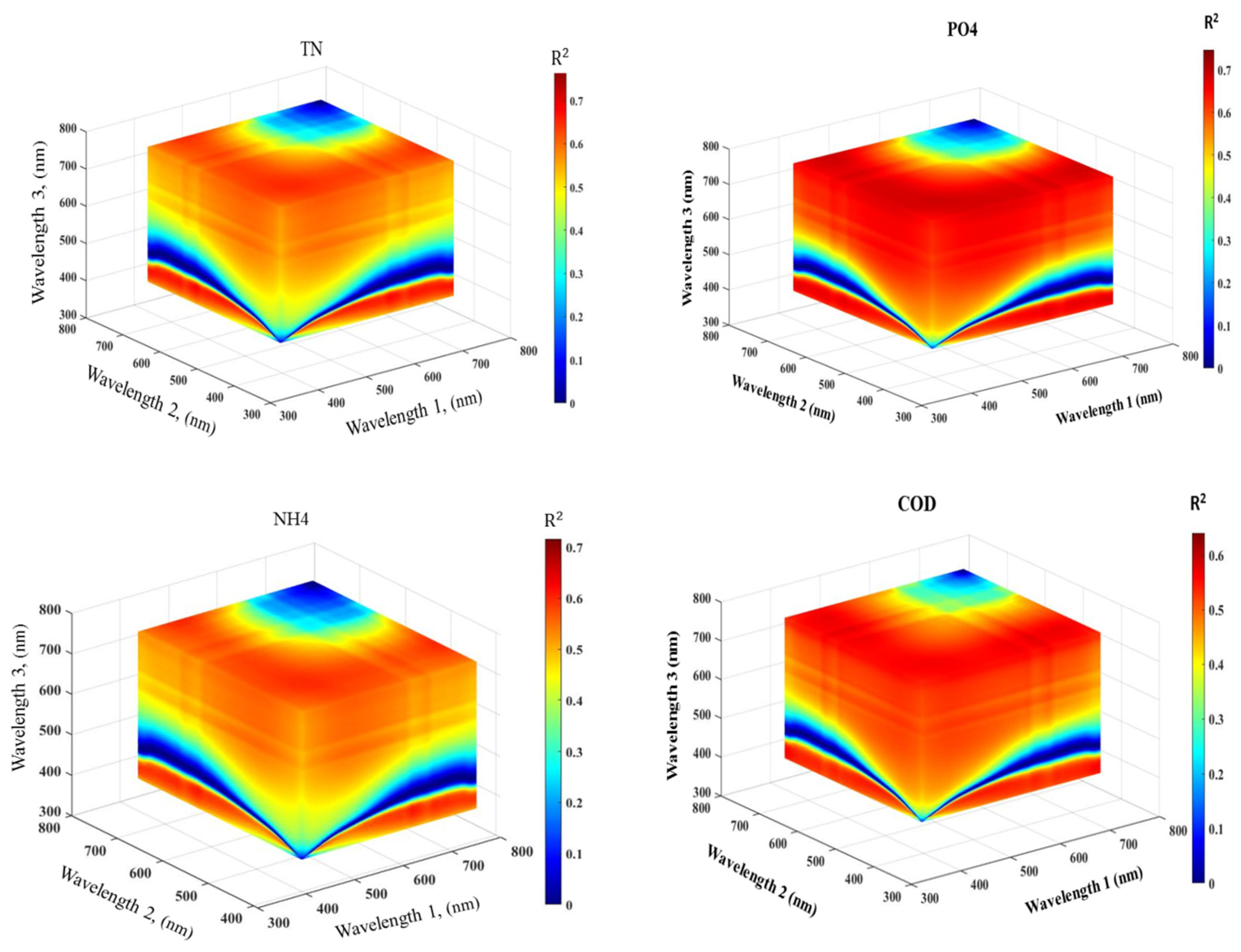
3.2. Variation Values of Different Types of Spectral Reflectance Indices

Changes in shallow lake systems may be detected by means of remotely sensed data in a non-destructive manner in order to estimate spatial variations across the entire lake. In the literature, several previous studies suggested that spectral-based indices derived from ground-based remote sensing measurements can be used to estimate spatial variations in WQPs [26,27,28,29,30]. Here, we investigate whether different groups of SRIs would be a useful tool for determining the water quality status of Lake Qaroun in terms of various WQPs. We also explored the efficiency of newly derived and published indices for the identification of WQPs at different stations in a two-year investigation (2018 and 2019).

The characteristics of the light reflected from water bodies at different wavebands along the magnetic spectrum can be used as indicators for the changes in the water’s physical and chemical composition [25,30,70,71]. Surprisingly, these changes cause significant shifts in the SRIs acquired from the water samples across the whole spectral range at specific bands. All tested spectral indices (PSRIs, NSRIs-2b, and NSRIs-3b), extracted as indicators of various WQPs, are presented in

Table 5. Variation values of 18 SRIs of water samples as averaged over two years for sixteen surface water samples.

	RSI700,560	RSI700,675	NDSI699,705,670,677	RSI833,1004	NDSI560,520	RSI622,602	RSI690,650	RSI760,484	RSI700,650
Site1	0.947 a–c	0.977 a–c	−5.689 a	2.938 a	0.022 a–c	0.9991 a–e	0.991 ab	0.798 a–c	0.972 a–c
Site2	0.971 a	0.988 a	3.295 a	2.294 ab	0.034 ab	1.010 a	0.9928 a	0.849 a	0.979 a
Site3	0.940 a–d	0.971 b–d	9.377 a	1.460 b–d	0.026 a–c	1.000 a–d	0.982 a–d	0.762 a–d	0.962 c–e
Site4	0.944 a–d	0.981 ab	−3.519 a	2.0432 bc	0.026 a–c	1.003 a–c	0.993 a	0.815 ab	0.978 ab
Site5	0.973 a	0.973 b–d	6.741 a	1.491 b–d	0.036 a	1.009 ab	0.987 a–c	0.820 ab	0.964 b–d
Site6	0.950 a–c	0.975 a–d	8.117 a	1.355 bc	0.024 a–c	1.003 a–c	0.983 a–d	0.776 a–d	0.965 b–d
Site7	0.958 ab	0.972 b–d	7.993 a	1.335 bc	0.029 a–c	1.002 a–c	0.980 b–e	0.785 a–d	0.960 c–f
Site8	0.881 c–e	0.967 b–d	4.082 a	1.866 b–d	0.007 cd	0.995 b–f	0.977 c–f	0.677 c–e	0.954 d–g
Site9	0.910 a–e	0.966 cd	4.291 a	1.273 bc	0.011 b–d	0.9999 a–e	0.979 c–f	0.702 b–e	0.955 d–g
Site10	0.840 e	0.962 d	3.251 a	1.178 bc	−0.013 d	0.990 c–f	0.971 d–f	0.587 e	0.946 fg
Site11	0.870 d,e	0.966 cd	5.669 a	1.260 bc	−0.007 d	0.991 c–f	0.971 d–f	0.617 e	0.949 e–g
Site12	0.899 a–e	0.971 b–d	8.000 a	1.666 b–d	0.006 cd	0.986 ef	0.969 ef	0.670 de	0.950 e–g
Site13	0.893 b–e	0.968 b–d	4.651 a	1.308 bc	0.008 cd	0.992 c–f	0.974 c–f	0.685 c–e	0.953 d–g
Site14	0.857 e	0.966 cd	4.569 a	1.057 d	−0.009 d	0.984 f	0.969 ef	0.606 e	0.947 fg
Site15	0.851 e	0.964 cd	4.901 a	1.176 bc	−0.010 d	0.986 ef	0.968 ef	0.594 e	0.945 g
Site16	0.842 e	0.962 d	4.341 a	0.984 d	−0.011 d	0.984 f	0.967 f	0.583 e	0.943 g
	RSI1130,500	NDSI620,610,622	NDSI700,648,712	NDSI648,712,696	NDSI698,650,712	NDSI620,614,602	NDSI620,600,614	NDSI620,600,614	NDSI696,710,652
Site1	1.125 a–c	−0.3332 a–c	−0.331 a-c	−0.3315 ab	−0.3277 ab	−0.3293 ab	−0.3335 a–d	−0.3338 a–d	−0.3328 e
Site2	1.145 ab	−0.3322 a	−0.3301 a	−0.3303 a	−0.3271 a	−0.3284 a	−0.3309 a	−0.3311 a	−0.3327 de
Site3	1.102 a–c	−0.3332 a–c	−0.3326 b–e	−0.3327 a–d	−0.3284 a–c	−0.3303 a–d	−0.3333 a–c	−0.3336 a–d	−0.3325 de
Site4	1.101 a–c	−0.333 ab	−0.3306 ab	−0.3307 b	−0.3274 ab	−0.3289 a	−0.3328 ab	−0.3331 a–c	−0.3324 de
Site5	1.175 a	−0.3327 ab	−0.3317 a–d	−0.332 a–c	−0.3274 ab	−0.3294 a–c	−0.3313 a	−0.3312 a	−0.3324 de
Site6	1.085 a–d	−0.3329 ab	−0.3325 b–e	−0.3327 a–d	−0.3288 a–d	−0.3304 a–e	−0.3325 ab	−0.3327 ab	−0.3322 c–e
Site7	1.118 a–c	−0.3333 a–c	−0.333 c–f	−0.3333 b–e	−0.3287 a–d	−0.3307 a–e	−0.333 a–c	−0.333 a–c	−0.3319 c–e
Site8	1.046 b–e	−0.3338 b–d	−0.3341 eg	−0.3346 c–g	−0.3295 b–e	−0.3317 c–f	−0.335 b–f	−0.335 b–e	−0.331 b–e
Site9	1.077 a–d	−0.3339 b–e	−0.3338 d–g	−0.3343 c–f	−0.3292 a–e	−0.3313 b–f	−0.334 a–e	−0.334 a–d	−0.3305 a–d
Site10	0.997 de	−0.3345 c–f	−0.3356 g	−0.3362 fg	−0.331 de	−0.3331 f	−0.3366 c–f	−0.337 c–e	−0.3302 a–c
Site11	0.986 de	−0.3340 b–f	−0.3352 fg	−0.3354 e–g	−0.3307 c–e	−0.3327 ef	−0.3361 b–f	−0.3367 b–e	−0.3301 a–c
Site12	0.995 de	−0.3348 d–f	−0.3355 g	−0.3359 fg	−0.3312 e	−0.3332 f	−0.3371 d–f	−0.3377 de	−0.3301 a–c
Site13	1.029 c–e	−0.3341 b–f	−0.3349 eg	−0.3353 d–g	−0.3305 c–e	−0.3325 d–f	−0.3357 b–f	−0.336 b–e	−0.3291 ab
Site14	0.966 e	−0.3352 ef	−0.3358 g	−0.3364 fg	−0.3312 e	−0.3333 f	−0.3381 f	−0.3386 e	−0.329 ab
Site15	0.966 e	−0.3349 d–f	−0.3359 g	−0.3364 fg	−0.3314 e	−0.3334 f	−0.3376 ef	−0.3382 e	−0.329 ab
Site16	0.986 de	−0.3354 f	−0.3362 g	−0.3369 g	−0.3314 e	−0.3336 f	−0.3383 f	−0.3387 e	−0.3286 a

The same letters are not statistically different from one another, according to Duncan’s test at a p-value of 0.05.

. The values of different SRIs demonstrated remarkable significant changes at different points of the shipboard survey throughout the entire lake (stations 1 to 16). Generally, when derived SRIs were linked to assess WQPs, the SRIs presented significant differences among nominated measuring stations. There were obvious differences between SRIs values among different stations, as seen in Table 5, which may have been a result of the great variations in WQPs at the same stations. For example, quantitative analyses revealed that the TN, NH₄⁺, PO₄³⁻ and COD values in Table 3 changed from 0.51 to 14.70, from 0.04 to 6.64, from 0.030 to 0.178, and from 23.88 to 44.52, respectively, and were then followed by changes in the values of NDSI_698,650,712, NDSI_620,614,602, NDSI_620,600,614 and NDSI_696,710,652 from −0.3336 to −0.3284, from −0.3383 to −0.3309, from−0.3387 to −0.3311, and from −0.3328 to −0.3286, as seen in Table 5. A gradual increase or decrease in the SRIs values associated with the variation in the values of WQPs across the lake was clearly noted.

3.3. Performance of Different SRIs to Asess WQPs

The R² for the relationships between the four WQPs and the SRIs was selected from the two and three-band slice map. The 2D maps, depicted in Figure 4, were derived from all potential combinations of binary dual wavelengths in the entire spectral range (302–1148 nm), while the 3D maps, illustrated in Figure 5, were derived using all possible combinations of binary dual wavelengths ranging from 390 to 750 nm. The best associations between the SRIs and WQPs were identified by the hotspot areas, based on the color scale for the best R². Based on the information gathered from the WQPs in the VIS, red-edge, and NIR regions, the NSRIs-2b and NSRIs-3b were selected based on the hotspots (color scale) of the discovered best R².

Table 6. Determination coefficients (R²) values for the relationship among 18 SRIs and total nitrogen (TN), ammonium (NH₄⁺), orthophosphate (PO₄³⁻), and chemical oxygen demand (COD) over two years.

SRIs	TN	NH4+	PO43−	COD
RSI700,560	0.59 ***	0.56 ***	0.62 ***	0.45 **
RSI700,675	0.36 **	0.29 *	0.35 **	0.35 **
NDSI699,705,670,677	0.00	0.00	0.01	0.03
RSI850,550	0.25 *	0.20 *	0.30 *	0.21 *
NDSI560,520	0.62 ***	0.59 ***	0.66 **	0.50 **
RSI622,602	0.73 ***	0.69 ***	0.64 ***	0.51 **
RSI690,650	0.71 ***	0.62 ***	0.68 ***	0.61 ***
RSI760,484	0.65 ***	0.60 ***	0.68 ***	0.55 ***
RSI700,650	0.63 ***	0.54 **	0.62 ***	0.58 ***
RSI1130,500	0.70 ***	0.66 ***	0.70 ***	0.51 **
NDSI610,614,608	0.74 ***	0.71 ***	0.63 ***	0.53 **
NDSI700,650,712	0.75 ***	0.66 ***	0.73 ***	0.64 ***
NDSI700,648,712	0.75 ***	0.65 ***	0.72 ***	0.64 ***
NDSI648,712,696	0.77 ***	0.69 ***	0.74 ***	0.63 ***
NDSI698,650,712	0.77 ***	0.68 ***	0.74 ***	0.64 ***
NDSI620,614,602	0.75 ***	0.72 ***	0.67 ***	0.53 **
NDSI620,600,614	0.74 ***	0.71 ***	0.66 ***	0.52 **
NDSI696,710,652	0.77 ***	0.69 ***	0.75 ***	0.62 ***

Levels of significance: *: p-value < 0.05, **: p-value < 0.01, and ***: p-value < 0.001.

shows the R² values for the association between the four measured WQPs and PSRIs (NSRIs-2b and NSRIs-3b).

Linear regression models revealed the most significant associations for the majority of SRIs combined with TN (R² = 0.25–0. 77), with NH₄⁺ (R² = 0.20–0.72), with PO₄³⁻ (R² = 0.30–0.75), and with COD (R² = 0.21–0.64). In general, the most of the PSRIs showed weak to moderate relationships with the four WQPs (TN, NH₄⁺, PO₄³⁻, and COD) (R² ranging from 0.45 to 0.64), while most of the NSRIs-2b showed moderate to strong relationships with three WQPs (TN, NH₄⁺, and PO₄³⁻) (R² = 0.54 to 0.73), and a moderate relationship with COD (R² = 0.51 to 0.61). The results further showed that the most of NSRIs-3b performed strong significant relationships with three WQPs (TN, NH₄⁺, and PO₄³⁻) (R² = 0.70 to 0.77), and a moderate relationship with COD (R² = 0.52 to 0.64), as detailed in Table 6. The newly constructed NSRIs-2b and NSRIs-3b were comparable to PSRIs, since the lowest R² always recorded with PSRIs for the relationships with WQPs. The relationships observed between TN and different SRIs recorded the highest coefficient of determination (R² = 0.77) with the NSRIs-3b (NDSI_648,712,696, NDSI_698,650,712 and NDSI_696,710,652); for the relationship between NH₄⁺ and different SRIs, the highest coefficient of determination (R² = 0.72) was recorded with the NSRIs-3b (NDSI_620,614,602); for the relationship between PO₄³⁻ and different SRIs, the highest coefficient of determination (R² = 0.75) was recorded with the NSRIs-3b (NDSI_696,710,652); and for the relationship between COD and different SRIs, the highest coefficient of determination (R² = 0.64) was recorded with the NSRIs-3b (NDSI_700,650,712, NDSI_700,648,712 and NDSI_698,650,712) in Table 6. In this study, the spectral index based on the electromagnetic spectrum’s red-edge regions appears to always produce a greater coefficient of determination. This could be explained by the red region of the electromagnetic spectrum being more sensitive to changes in TN. Liu et al. [28] performed a correlation analysis between the hyperspectral reflectance and the measured TN, and discovered that spectral index calculated from wavelengths near 680, 850, and 940 nm could be used as a sensitivity indicator for the inversion of total TN in surface water. Moreover, since the chlorophyll is strongly related to TN, Elhag et al. [28] revealed that the maximum chlorophyll index (MCI) calculated from wavelengths of 665, 705, and 740 nm from the red-edge regions could be utilized to estimate chlorophyll concentrations in water. In addition, Liu et al. [72] found that Band 3 (red region: 630–700 nm) of IKONOS presented a strong relationship with TN in an urban water surface in China, with an R² of 0.87

Orthophosphates are one of the most important plant nutrients, as they aid in the rapid growth of plants and algae. The concentration of Chl-a is proportional to total phosphorus [4]. The NDSI_696,710,652 index, which was used to estimate TN, presented a strong relationship with PO₄³⁻ (R² = 0.75). Shafique et al. [68] reported that the spectral index (R₅₅₄/R₆₇₅), calculated from green and red regions, was sensitive to phosphorus concentrations with R² = 0.59. In this study, most of the indices, including the wavelength from green and red regions, could be used to estimate PO₄³⁻. Other studies have demonstrated that spectral reflectance indices based on the blue (450–510 nm) and green (500–600 nm) regions are very sensitive to variations in total phosphorus concentrations in water [73,74,75]. One of the most important pollutant variables in water (chemical oxygen demand (COD) alters light radiation by changing its absorption and scattering characteristics, resulting in different characteristic absorption spectra that are strongly correlated with pollutant level and spectral reflectance. In this study, the most of spectral indices of two- and three-band presented significant relationships with the R² varied from 0.21 to o.64. the most of NSRIs-2b and NSRIs-3 which included the wavelength from green or red, or both, which could be used to assess COD.

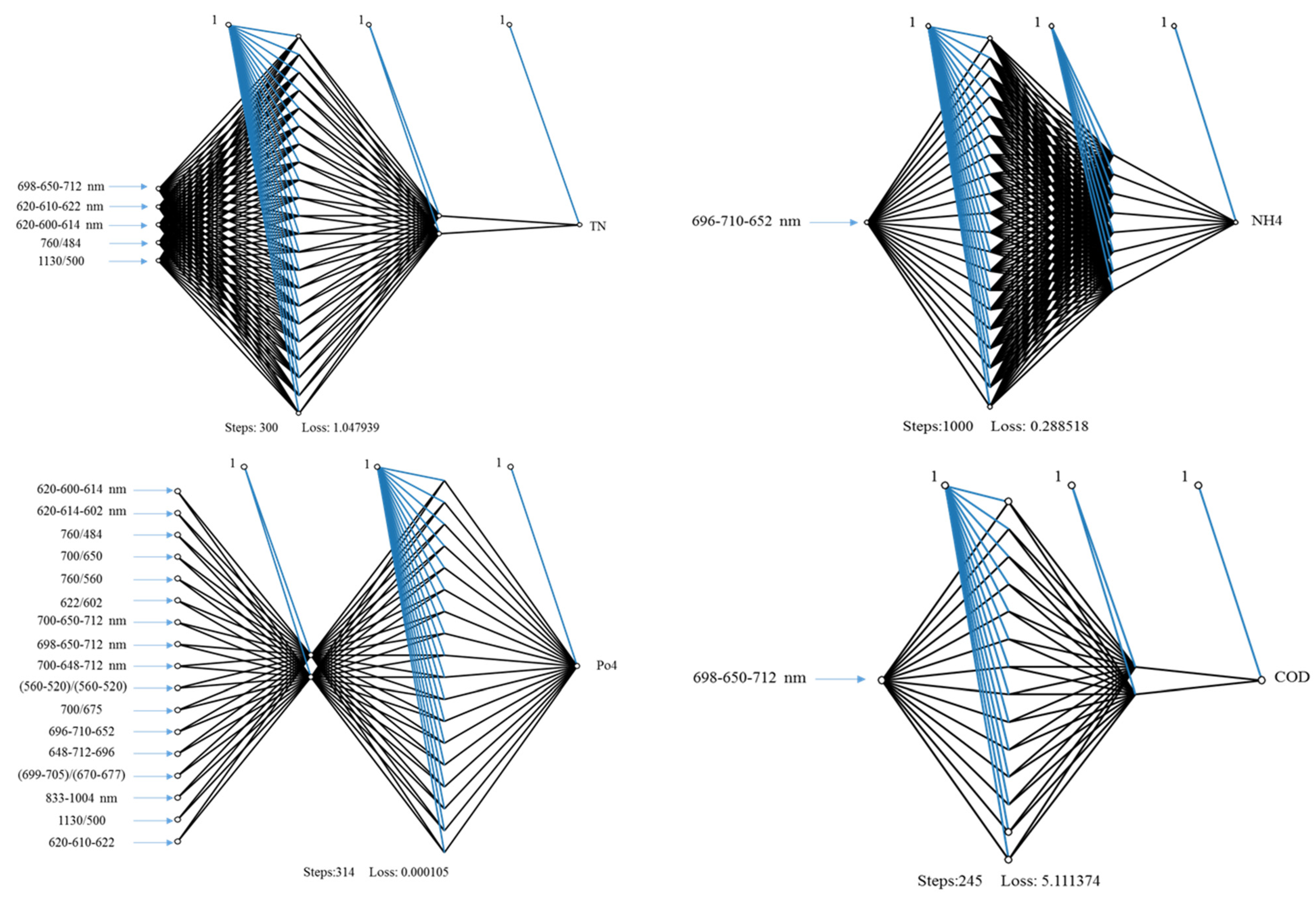
3.4. Performance of Artificial Neural Networks Based on SRIs to Asess WQPs

The neural network architectures after gathering senior 3D-VI features are illustrated in Figure 6. The figure showed the best neural network structure with the variants chosen. Every network topology offers basic data, such as the synaptic weights trained on a range of hidden neuron layers, steps for converging, and the overall errors. The network topology is constructed with a specific combination of input parameters, with a number of hidden neuron layers and different activation functions. For instance, the model of ANN-TN-VI-5 had hidden neuron layers (22, 2) at the ReLu function, ANN- NH₄⁺-VI-1 needed (20, 8) at the logistic function, ANN- PO₄³⁻VI-17 required (2, 18) at the tanh function, and ANN-COD-VI-1 chosen (14, 2) at the tanh function. The layout presented in Figure 6 depicts advanced models for estimating TN, NH₄⁺, PO₄³⁻, and COD. The calibrating process obligated 300, 1000, 314, and 245 steps, respectively for achieving a lower error function. The process has an overall error rate of roughly 1.047, 0.289, 0.00011, and 5.111, respectively. The expected performance was improved as noted by Thawornwong and Enke [76]; to avoid over-fitting, the network was trained by the back-propagation mathematical algorithm with early stopping.

From the results, the 3D vegetation indices (VI) were the premium integration to filter the uppermost variables. These indices had a high ranking for measuring the considered parameters of the water. The neural network was trained with the super indices features (independent variables) for predicting the studied parameters (dependent variable). The expected values were then compared with the reserved values not implemented for the neural network. This study evaluated multivariate methods, and compared the results clearly, so the use of multivariate methods greatly enhanced predictability. Independent validation can also be considered the most reliable method for assessing the accuracy of the regression model, since validation data are not involved in the model development process. The ANN-TN-VI-5 was the optimum predictive model, as evidenced by the performance, and showed a stronger relationship between the superlative features and TN. The five features involved in this model are of great significance for predicting TN. Its outputs with R² were 0.92 (calibration) and 0.84 (validation), as listed in

Table 7. Results of calibration and validation models of artificial neural networks of the association between spectral reflectance indices and total nitrogen (TN), ammonium (NH₄⁺), orthophosphate (PO₄³⁻), and chemical oxygen demand (COD).

WQPs	Parameters	Indices	Calibration	Validation
			R2	R2	RMSE
TN	(22, 2), ReLu	DSI698,650,712; NDSI620,610,622; NDSI620,600,614; RSI760,48; RSI1130,500	0.92 ***	0.84 ***	1.558
NH4+	(20, 8) logistic	DSI696,710,652	0.97 ***	0.80 ***	0.695
PO43−	(2, 18) tanh	NDSI620,600,614; NDSI620,614,602; RSI760,484; RSI700,650; RSI700,560; RSI622,602; NDSI700,650,712; NDSI698,650,712; NDSI700,648,712; NDSI560,520; RSI700,675; NDSI696,710,652; NDSI648,712,696; NDSI699,705,670,677; RSI833,1004; RSI1130,500; NDSI620,610,622	0.98 ***	0.89 ***	0.014
COD	(14, 2) tanh	DSI698,650,712	0.79 ***	0.66 ***	2.644

Levels of significance: ***: p < 0.001.

. The ANN-NH₄⁺-VI-1 model was ranked first in performance to measure NH₄⁺. The R² value was 0.968 and 0.798 in the training and validation datasets, respectively. The ANN-PO₄³⁻-VI-17 was the highest accurate model for observing PO₄³⁻ (R² = 0.98 and 0.89 for calibration and validation, respectively). The model ANN-COD-VI-1 constructed for determining COD had higher performance expectations (R² = 0.79 and 0.66 for calibration and validation, respectively), as presented in Table 7. The expected performance was improved, as demonstrated by Elsherbiny et al. [77]; to upgrade the regression algorithms for robust prediction, some actions were required during training, such as filtering high-level features and optimizing hyperparameters of the model. Lui et al. [72] found that IKONOS imagery data coupled with ANNs models could be used to estimate TN and TP concentrations with R² = 0.98 and 0.94, respectively.

4. Advantages and Limitations of Our Research and Expected Future Work

Among surface water resources, lakes play a vital role in water supply for different purposes (agriculture, industry, and domestic uses) in many regions worldwide. The WQPs of a lake will be drastically altered as a result of predicted global warming, making it necessary to monitor and assess WQPs of the lake ecosystem in order to conserve life across the entire lake, necessitating the use of increasingly advanced monitoring tools. In this regard, it is argued that spatially resolved, regional-scale data obtained using remote sensing techniques would be reliable in lake monitoring. The findings of our research revealed that ground-based spectral indices have been shown as a useful tool for predicting and assessing various WQPs, but this is on a small-scale, and needs to be extrapolated using satellite data. Using ground-based remote sensing data, researchers were able to characterize spatio-temporal variability at the lake scale, allowing point-sampling procedures to be extrapolated to the larger ecosystem. As a result, remote sensing data can make a significant contribution to the interpretation of lake function, and hence will be indirectly valuable to the general public. Using ground-based remote sensing measurements, it was shown that precise estimation of WQPs is possible. One of the limitations to our research was obtaining high spatial and high spectral satellite images in order to extrapolate the results at a regional scale. Due to the lack of spatial and spectral resolution capacities of satellite imagery until the first decade of the 21st century, plus a high total cost, it was not easy to use satellite imagery in assessing WQPs. Clouds can obscure ground features, data may not be captured at important moments, and users may have to sift through a large number of images to obtain meaningful information. The ANN model provides good advantages to increase the prediction of WQPs more than spectral indices, since ANN models can include several spectra bands or several spectral indices derived from different spectrum regions.

For future investigations, a combined methods of ground- and satellite-based remote sensing in the evaluation of water status in lakes would be an efficient technique. With the aid of recently launched hyperspectral satellites, which have a decent number of spectral bands, it would be easy to assess WQPs on a regional scale via calculating the great number of two- and three- band indices, based on satellite data. From an economic standpoint, combining satellite and ground-based datasets will be comparable to the sampling-point technique in terms of overall cost. These technologies may open an avenue for rapid, high-resolution assessments of lakes’ ecological conditions, as well as being equally important for furthering the understanding of lake-scale process and function.

5. Conclusions

This research study examined the efficiency of ground-based remote sensing based spectral indices for the retrieval of different WQPs, including total nitrogen (TN), ammonium (NH₄⁺), orthophosphate (PO₄³⁻), and chemical oxygen demand (COD), using hyperspectral data collected from multi-temporal cruises over a two-year campaign (2018 and 2019). The distribution patterns of four different WQPs using GIS maps demonstrated that the WQPs are contaminated to varying degrees. In the present study, different PSRIs, NSRIs-2b and NSRIs-3b, as well as ANNs were used for the quantification of some WQPs of Lake Qaroun. The results showed that all NSRIs-3b presented stronger relationships for estimating WQPs, compared to other SRIs. For instance, the NSRIs-3b (NDSI_696,710,652) produced the highest relationships with TN and PO₄³⁻, with respective R² values = of 0.77, and 0.75. In both the calibration and validation datasets, the results revealed that ANN algorithm models based on all SRIs performed best for estimating WQPs. For instance, the five features involved in this model are of great significance for predicting TN. Its outputs showed high R² values of 0.92 and 0.84 for calibration and validation, respectively. In conclusion, this research suggests that integrating SRIs with ANNs would be a promising and accurate method for the quantification of different WQPs in Lake Qaroun.

References

1. Poonam, T.; Tanushree, B.; Sukalyan, C. Water quality indices—Important tools for water quality assessment, a review. Int. J. Adv. Chem. 2013, 1, 15–29. [Google Scholar]
2. Ismail, A.H.; Abed, B.S.H.; Abdul-Qader, S. Application of multivariate statistical techniques in the surface water quality assessment of Tigris River at Baghdad stretch, Iraq. J. Babylon Univ./Eng. Sci. 2014, 2, 450–462. [Google Scholar]
3. Herojeet, R.K.; Rishi, M.S.; Lata, R.; Sharma, R. Application of environmetrics statistical models and water quality index for groundwater and water quality index for groundwater quality characterization of alluvial aquifer of Nalagarh Valley, Himachal Pradesh, India. Sustain. Water Resour. Manag. 2016, 2, 39–53. [Google Scholar] [CrossRef] [Green Version]
4. Tirkey, P.; Bhattacharya, T.; Chakraborty, S. Water Quality Indices—Important tools for water quality assessment: A Review. Int. J. Adv. Chem. 2015, 1, 15–29. [Google Scholar]
5. Nagy-Kovács, Z.; Davidesz, J.; Czihat-Mártonné, K.; Till, G.; Fleit, E.; Grischek, T. Water Quality Changes during Riverbank Filtration in Budapest, Hungary. Water 2019, 11, 302. [Google Scholar] [CrossRef] [Green Version]
6. Sandhu, C.; Grischek, T.; Börnick, H.; Feller, J.; Sharma, S.K. A Water Quality Appraisal of Some Existing and Potential Riverbank Filtration Sites in India. Water 2019, 11, 215. [Google Scholar] [CrossRef] [Green Version]
7. El-Batrawy, O.A.; Ibrahim, M.S.; Fakhry, H.; El-Aassar, M.R.; El-Zeiny, A.M.; El-Hamid, H.T.A.; El-Alfy, M.A. Anthropogenic Impacts on Water Quality of River Nile and Marine Environment, Rosetta Branch Using Geospatial Analyses. J. Environ. Sci. 2018, 47, 89–101. [Google Scholar]
8. USEPA. National Recommended Water Quality Criteria; Office of Water, United States Environmental Protection Agency: Washington, DC, USA, 2018.
9. UNEP. United Nations Environment Programme. UNEP Frontiers 2018/19 Report: Emerging Issues of Environmental Concern; UNEP: Nairobi, Kenya, 2019. [Google Scholar]
10. Edokpayi, J.N.; Odiyo, J.O.; Durowoju, O.S. Impact of Wastewater on Surface Water Quality in Developing Countries: A Case Study of South Africa. Water Quality, Hlanganani Tutu. In Water Quality; InTechOpen: Rijeka, Croatia, 2017; pp. 401–416. [Google Scholar]
11. Ssekyanzi, A.; Nevejan, N.; Van der Zande, D.; Brown, M.E.; Van Stappen, G. Identification of Potential Surface Water Resources for Inland Aquaculture from Sentinel-2 Images of the Rwenzori Region of Uganda. Water 2021, 13, 2657. [Google Scholar] [CrossRef]
12. El-Zeiny, A.M.; El Kafrawy, S.B.; Ahmed, M.H. Geomatics based approach for assessing Qaroun Lake pollution, Egypt. J. Remote Sens. Space Sci. 2019, 22, 279–296. [Google Scholar]
13. Ali, M.H.H.; Abdel-Satar, A.M.; Goher, M. Present Status and Long-Term Changes of Water Quality Characteristics in Heavily Polluted Mediterranean Lagoon, Lake Mariut, Egypt. IJRDO-J. Appl. Sci. 2017, 3, 66–82. [Google Scholar]
14. El-Sayed, S.A.; Hassan, H.B.; El-Sabagh, M.E.I. Geochemistry and mineralogy of Qaroun Lake and relevant drain sediments, El-Fayoum, Egypt. J. Afr. Earth Sci. 2021, 185, 104388. [Google Scholar] [CrossRef]
15. Usali, N.; Ismail, M.H. Use of remote sensing and gis in monitoring water quality. J. Sustain. Dev. 2010, 3, 228–238. [Google Scholar] [CrossRef]
16. Varol, M. Use of water quality index and multivariate statistical methods for the evaluation of water quality of a stream affected by multiple stressors: A case study. Environ. Pollut. 2020, 266, 115417. [Google Scholar] [CrossRef] [PubMed]
17. Goher, M.E.; Mahdy, E.M.; Abdo, M.H.; El Dars, F.M.; Korium, M.A.; Elsherif, A.S. Water quality status and pollution indices of Wadi El-Rayan lakes, El-Fayoum, Egypt. Sustain. Water Resour. Manag. 2019, 5, 387–400. [Google Scholar] [CrossRef]
18. Abdel-Satar, A.M.; Ali, M.H.; Goher, M.E. Indices of water quality and metal pollution of Nile River, Egypt. Egypt. J. Aquat. Res. 2017, 43, 21–29. [Google Scholar] [CrossRef]
19. Davis, A.P.; McCuen, R.H. Storm Water Management for Smart Growth, 1st ed.; Springer Science and Business Media: New York, NY, USA, 2005. [Google Scholar]
20. Sutadian, A.D.; Muttil, N.; Yilmaz, A.G.; Perera, B.J.C. Development of river water quality indices—A review. Environ. Monit. Assess. 2016, 188, 58. [Google Scholar] [CrossRef] [Green Version]
21. Abdelmalik, K. Role of statistical remote sensing for Inland water quality parameters prediction. Egypt. J. Remote Sens. Space Sci. 2018, 21, 193–200. [Google Scholar] [CrossRef]
22. Noori, R.; Karbassi, A.R.; Mehdizadeh, H.; Vesali-Naseh, M.; Sabahi, M.S.A. Framework development for predicting the longitudinal dispersion coefficient in natural streams using an artificial neural network. Environ. Prog. Sustain. Energy 2011, 30, 439–449. [Google Scholar] [CrossRef]
23. Modabberi, A.; Noori, R.; Madani, K.; Ehsani, A.H.; Mehr, A.D.; Hooshyaripor, F.; Kløve, B. Caspian Sea is eutrophying: The alarming message of satellite data. Environ. Res. Lett. 2020, 15, 124047. [Google Scholar] [CrossRef]
24. Abd-Elrahman, A.; Croxton, M.; Pande-Chettri, R.; Toor, G.S.; Smith, S.; Hill, J. In situ estimation of water quality parameters in freshwater aquaculture ponds using hyperspectral imaging system. ISPRSJ Photogramm. Remote Sens. 2011, 66, 463–472. [Google Scholar] [CrossRef]
25. Vinciková, H.; Hanuš, J.; Pechar, L. Spectral reflectance is a reliable water-quality estimator for small, highly turbid wetlands. Wetlands Ecol. Manag. 2015, 23, 933–946. [Google Scholar] [CrossRef]
26. Han, L.; Jordan, K.J. Estimating and mapping chlorophyll-a concentration in Pensacola Bay, Florida using Landsat ETM+ data. Int. J. Remote Sens. 2005, 26, 5245–5254. [Google Scholar] [CrossRef]
27. Wang, Z.; Kawamura, K.; Sakuno, Y.; Fan, X.; Gong, Z.; Lim, J. Retrieval of chlorophyll-a and total suspended solids using iterative stepwise elimination partial least squares (ISE-PLS) regression based on field hyperspectral measurements in irrigation ponds in Higashihiroshima, Japan. Remote Sens. 2017, 9, 264. [Google Scholar] [CrossRef] [Green Version]
28. Elhag, M.; Gitas, I.; Othman, A.; Bahrawi, J.; Gikas, P. Assessment of water quality parameters using temporal remote sensing spectral reflectance in arid environments, Saudi Arabia. Water 2019, 11, 556. [Google Scholar] [CrossRef] [Green Version]
29. Liu, C.; Zhang, F.; Ge, X.; Zhang, X.; Chan, N.W.; Qi, Z. Measurement of total nitrogen concentration in surface water using hyperspectral band observation method. Water 2020, 12, 1842. [Google Scholar] [CrossRef]
30. Elsayed, S.; Gad, M.; Farouk, M.; Saleh, A.H.; Hussein, H.; Elmetwalli, A.H.; Elsherbiny, O.; Moghanm, F.S.; Moustapha, M.E.; Taher, M.A.; et al. Using optimized two and three-band spectral indices and multivariate models to assess some water quality indicators of Qaroun Lake in Egypt. Sustainability 2021, 13, 10408. [Google Scholar] [CrossRef]
31. Lindell, T.; Pierson, D.; Premazzi, G.; Zilioli, E. Manual for Monitoring European Lakes Using Remote Sensing Techniques; European Commission Joint Research Centre: Ispra, Italy, 1999. [Google Scholar]
32. Sarkar, A.; Pandey, P. River water quality modelling using artificial neural network technique. Aquat. Procedia 2015, 4, 1070–1077. [Google Scholar] [CrossRef]
33. Isiyaka, H.A.; Mustapha, A.; Juahir, H.; Phil-Eze, P. Water quality modelling using artificial neural network and multivariate statistical techniques. Model. Earth Syst. Environ. 2019, 5, 583–593. [Google Scholar] [CrossRef]
34. Adnan, R.M.; Liang, Z.; El-Shafie, A.; Zounemat-Kermani, M.; Kisi, O. Daily streamflow prediction using optimally pruned extreme learning machine. J. Hydrol. 2019, 577, 123981. [Google Scholar] [CrossRef]
35. Šiljić Tomić, A.; Antanasijević, D.; Ristić, M.; Perić-Grujić, A.; Pocajt, V. Application of experimental design for the optimization of artificial neural network-based water quality model: A case study of dissolved oxygen prediction. Environ. Sci. Pollut. Res. Int. 2018, 25, 9360–9370. [Google Scholar] [CrossRef] [PubMed]
36. Attia, A.H.; El-Sayed, S.A.; El-Sabagh, M.E. Utilization of GIS modeling in geoenvironmental studies of Qaroun Lake, El Fayoum Depression, Egypt. J. Afr. Earth Sci. 2018, 138, 58–74. [Google Scholar] [CrossRef]
37. Rawat, K.S.; Jacintha, T.G.A.; Singh, S.K. Hydro-chemical survey and quantifying spatial variations in groundwater quality in coastal region of Chennai, Tamilnadu, India—A case study. Indones. J. Geog. 2018, 50, 57–69. [Google Scholar] [CrossRef]
38. El-Sayed, S.A.; Moussa, E.M.M.; El-Sabagh, M.E.I. Evaluation of heavy metal content in Qaroun Lake, El-Fayoum, Egypt. Part I: Bottom sediments. J. Radiat. Res. Appl. Sci. 2015, 8, 276–285. [Google Scholar] [CrossRef] [Green Version]
39. Redwan, M.; Elhaddad, E. Heavy metals seasonal variability and distribution in Lake Qaroun sediments, El-Fayoum, Egypt. J. Afr. Earth Sci. 2017, 134, 48–55. [Google Scholar] [CrossRef]
40. Gad, M.; Abou El-Safa, M.M.; Farouk, M.; Hussein, H.; Alnemari, A.M.; Elsayed, S.; Khalifa, M.M.; Moghanm, F.S.; Eid, E.M.; Saleh, A.H. Integration of water quality indices and multivariate modeling for assessing Surface water quality in Qaroun Lake, Egypt. Water 2021, 13, 2258. [Google Scholar] [CrossRef]
41. Singh, S.K.; Srivastava, P.K.; Pandey, A.C.; Gautam, S.K. Integrated assessment of groundwater influenced by a confluence river system: Concurrence with remote sensing and geochemical modelling. Water Resour. Manag. 2013, 27, 4291–4313. [Google Scholar] [CrossRef]
42. Abowaly, M.E.; Belal, A.-A.A.; Abd Elkhalek, E.E.; Elsayed, S.; Abou Samra, R.M.; Alshammari, A.S.; Moghanm, F.S.; Shaltout, K.H.; Alamri, S.A.M.; Eid, E.M. Assessment of soil pollution levels in North Nile Delta, by integrating contamination indices, GIS, and multivariate modeling. Sustainability 2021, 13, 8027. [Google Scholar] [CrossRef]
43. Haykin, S. Neural Networks: A Comprehensive Foundation, 2nd ed.; Prentice Hall: Upper Saddle River, NJ, USA, 1999. [Google Scholar]
44. Li, J.; Yoder, R.; Odhiambo, L.O.; Zhang, J. Simulation of nitrate distribution under drip irrigation using artificial neural networks. Irrig. Sci. 2004, 23, 29–37. [Google Scholar] [CrossRef]
45. Khadr, M.; Gad, M.; El-Hendawy, S.; Al-Suhaibani, N.; Dewir, Y.H.; Tahir, M.U.; Mubushar, M.; Elsayed, S. The Integration of multivariate statistical approaches, hyperspectral reflectance, and data-driven modeling for assessing the quality and suitability of groundwater for irrigation. Water 2021, 13, 35. [Google Scholar] [CrossRef]
46. Schalkoff, J. Artificial Neural Networks; McGraw-Hill Companies Inc.: New York, NY, USA, 1997. [Google Scholar]
47. Byrd, R.H.; Lu, P.; Nocedal, J.; Zhu, C. A limited memory algorithm for bound constrained optimization. Siam J. Sci. Comput. 1995, 16, 1190–1208. [Google Scholar] [CrossRef]
48. Glorfeld, L.W. A methodology for simplification and interpretation of backpropagation-based neural network models. Expert Syst. Appl. 1996, 10, 37–54. [Google Scholar] [CrossRef]
49. Malone, B.P.; Styc, Q.; Minasny, B.; McBratney, A.B. Digital soil mapping of soil carbon at the farm scale: A spatial downscaling approach in consideration of measured and uncertain data. Geoderma 2017, 290, 91–99. [Google Scholar] [CrossRef]
50. Saggi, M.K.; Jain, S. Reference evapotranspiration estimation and modeling of the Punjab Northern India using deep learning. Comput. Electron. Agr. 2019, 156, 387–398. [Google Scholar] [CrossRef]
51. Menken, K.D.; Brezonik, P.L.; Bauer, M.E. Influence of chlorophyll and colored dissolved organic matter (CDOM) on Lake Reflectance Spectra: Implications for Measuring Lake Properties by Remote Sensing. Lake Reserv. Manag. 2006, 22, 179–190. [Google Scholar] [CrossRef] [Green Version]
52. Gitelson, A.; Yacobi, Y. Monitoring Quality of Productive Aquatic Ecosystem: Requirements for Satellite Sensors; BALWOIS: Ohrid, North Macedonia, 2004. [Google Scholar]
53. Kallio, K.; Kutser, T.; Hannonen, T.; Koponen, S.; Pulliainen, J.; Vepsalainen, J.; Pyhalahti, T. Retrieval of water quality from airborne imaging spectrometry of various lake types in different seasons. Sci. Total Environ. 2001, 268, 59–77. [Google Scholar] [CrossRef]
54. Sterckx, S.; Knaeps, E.; Bollen, M.; Trouw, K.; Houthuys, R. Retrieval of suspended sediment from advanced hyperspectral sensor data in the Scheldt estuary at different stages in the tidal cycle. Mar. Geod. 2007, 30, 97–108. [Google Scholar] [CrossRef]
55. Gitelson, A.; Szilagyi, F.; Mittenzwey, K.-H. Improving quantitative remote sensing for monitoring of inland water quality. Water Res. 1993, 27, 1185–1194. [Google Scholar] [CrossRef]
56. Taha, O.E.; Abd El-Monem, A.M. Phytoplankton composition, biomass and productivity in Wadi El-Rayian Lakes, Egypt. Conference on the role of science in the development of Egyptian society and environment. Zaga. Univ. Fac. Sci. 1999, 22, 48–56. [Google Scholar]
57. Khalifa, N. Population dynamics of Rotifera in Ismailia Canal, Egypt. J. Biodivers. Environ. Sci. 2014, 4, 58–67. [Google Scholar]
58. CCME (Canadian Council of Ministers of the Environment). For the protection of aquatic life. In Canadian Environmental Quality Guidelines; Canadian Council of Ministers of the Environment: Winnipeg, MB, Canada, 2007. [Google Scholar]
59. Hamid, A.; Bhat, S.A.; Jehangir, A. Local determinants influencing stream water quality. Appl. Water Sci. 2020, 10, 24. [Google Scholar] [CrossRef] [Green Version]
60. Singh, K.P.; Malik, A.; Mohan, D.; Sinha, S. Multivariate statistical techniques for the evaluation of spatial and temporal variations in water quality of Gomti River (India): A case study. Water Res. 2004, 38, 3980–3992. [Google Scholar] [CrossRef]
61. Wetzel, R.G. Limnology; Academic Press: London, UK, 2001; 1006p. [Google Scholar]
62. Sharip, Z.; Suratman, S. Formulating specific water quality criteria for lakes: A Malaysian perspective. In Water Quality; Tutu, H., Ed.; IntechOpen: Rijeka, Croatia, 2017; pp. 293–313. [Google Scholar]
63. Yazidi, A.; Saidi, S.; Ben Mbarek, N.; Darragi, F. Contribution of GIS to evaluate surface water pollution by heavy metals: Case of Ichkeul Lake (Northern Tunisia). J. Afr. Earth Sci. 2017, 134, 166–173. [Google Scholar] [CrossRef]
64. WHO. Guidelines for Drinking-Water Quality, 4th Edition, Incorporating the 1st Addendum; WHO: Geneva, Switzerland, 2017. [Google Scholar]
65. Penn, M.R.; Pauer, J.J.; Mihelcic, J.R. Environmental and Ecological Chemistry—Vol. II—Biochemical Oxygen Demand; Eolss Publishers: Oxford, UK, 2003. [Google Scholar]
66. Noori, R.; Ansari, E.; Jeong, Y.-W.; Aradpour, S.; Maghrebi, M.; Hosseinzadeh, M.; Bateni, S.M. Hyper-Nutrient Enrichment Status in the Sabalan Lake, Iran. Water 2021, 13, 2874. [Google Scholar] [CrossRef]
67. Noori, R.; Ansari, E.; Bhattarai, R.; Tang, Q.; Aradpour, S.; Maghrebi, M.; Haghighi, A.T.; Bengtsson, L.; Kløve, B. Complex dynamics of water quality mixing in a warm mono-mictic reservoir. Sci. Total Environ. 2021, 777, 146097. [Google Scholar] [CrossRef] [PubMed]
68. Kumar, M.R.; Kumar, R.V.; Sreejani, T.P.; Sravya, P.V.R.; Rao, G.S. Multivariate statistical analysis of water quality of Godavari River at Polavaram for irrigation purposes. In Water Resources and Environmental Engineering II; Springer: Singapore, 2019; pp. 115–124. [Google Scholar]
69. Zhao, Y.; Xia, X.H.; Yang, Z.F.; Wang, F. Assessment of water quality in Baiyangdian Lake using multivariate statistical techniques. Procedia Environ. Sci. 2012, 13, 1213–1226. [Google Scholar] [CrossRef] [Green Version]
70. Maliki, A.A.A.; Chabuk, A.; Sultan, M.A.; Hashim, B.M.; Hussain, H.M.; Al-Ansari, N. Estimation of total dissolved solids in water bodies by spectral indices Case Study: Shatt al-Arab River. Water Air Soil Pollut. 2020, 231, 482. [Google Scholar] [CrossRef]
71. Shafique, N.A.; Fulk, F.; Autrey, B.C.; Flotemersch, J. Hyperspectral remote sensing of water quality parameters for large rivers in the Ohio River Basin. In Proceedings of the First Interagency Conference on Research in the Watersheds, Benson, AZ, USA, 27–30 October 2003. [Google Scholar]
72. Liu, J.; Zhang, Y.; Yuan, D.; Song, X. Empirical estimation of total nitrogen and total phosphorus concentration of urban water bodies in China using high resolution IKONOS multispectral imagery. Water 2015, 7, 6551–6573. [Google Scholar] [CrossRef] [Green Version]
73. Gholizadeh, M.H.; Melesse, A.M.; Reddi, L.A. A Comprehensive review on water quality parameters estimation using remote sensing techniques. Sensors 2016, 16, 1298. [Google Scholar] [CrossRef] [PubMed] [Green Version]
74. Osinska-Skotak, K.; Kruk, M.; Mróz, M. The Spatial Diversification of Lake Water Quality Parameters in Mazurian Lakes in Summertime; Millpress: Rotterdam, The Netherlands, 2007. [Google Scholar]
75. Wu, C.; Wu, J.; Qi, J.; Zhang, L.; Huang, H.; Lou, L.; Chen, Y. Empirical estimation of total phosphorous concentration in the mainstream of the Qiantang River in China using Landsat TM data. Int. J. Remote Sens. 2010, 31, 2309–2324. [Google Scholar] [CrossRef]
76. Thawornwong, S.; Enke, D. The adaptive selection of financial and economic variables for use with artificial neural networks. Neurocomputing 2004, 56, 205–232. [Google Scholar] [CrossRef]
77. Elsherbiny, O.; Zhou, L.; Feng, L.; Qiu, Z. Integration of Visible and Thermal Imagery with an Artificial Neural Network Approach for Robust Forecasting of Canopy Water Content in Rice. Remote Sens. 2021, 13, 1785. [Google Scholar] [CrossRef]
Figure 1. Location map of Lake Qaroun and sampling stations throughout the entire lake. S is abbreviation of the site.
Water 13 03094 g001
Figure 2. WQPs spatial distribution maps of in 2018: (a) total nitrogen (TN), (b) ammonium (NH4+), (c) orthophosphate PO43−, and (d) chemical oxygen demand (COD).
Water 13 03094 g002
Figure 3. Spatial distribution maps of WQPs in 2019: (a) total nitrogen (TN), (b) ammonium (NH4+), (c) orthophosphate PO43−, and (d) chemical oxygen demand COD.
Water 13 03094 g003
Figure 4. Correlation matrices showing the determination coefficients (R2) values for potential combinations of each wavelength from 302 to 1148 nm with total nitrogen (TN), ammonium (NH4+), orthophosphate (PO43−), and chemical oxygen demand (COD) over two years.
Water 13 03094 g004
Figure 5. Three-dimensional slice map of the determination coefficients (R2) values that were obtained for the relationship between total nitrogen (TN), ammonium (NH4+), orthophosphate (PO43−), and chemical oxygen demand (COD) over two years that was calculated for all potential combinations of each three-band from 390–750 nm.
Water 13 03094 g005
Figure 6. Neural network diagrams for this study, including total nitrogen (TN), ammonium (NH4+), orthophosphate (PO43−), and chemical oxygen demand (COD).
Water 13 03094 g006