
Phycocyanin Monitoring in Some Spanish Water Bodies with Sentinel-2 Imagery

 , ,
, ,  , , ,
, , , 
Abstract
:1. Introduction
2. Materials and Methods
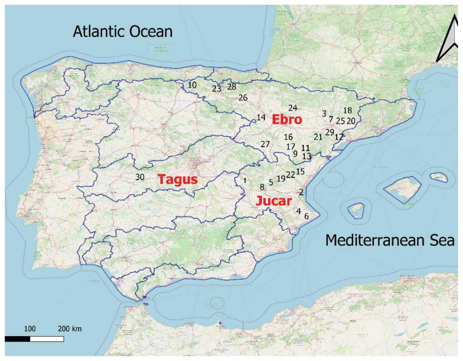
2.1. Study Site
2.2. Sampling Methods
2.3. Image Processing
2.4. Calibration
2.5. Validation
3. Results
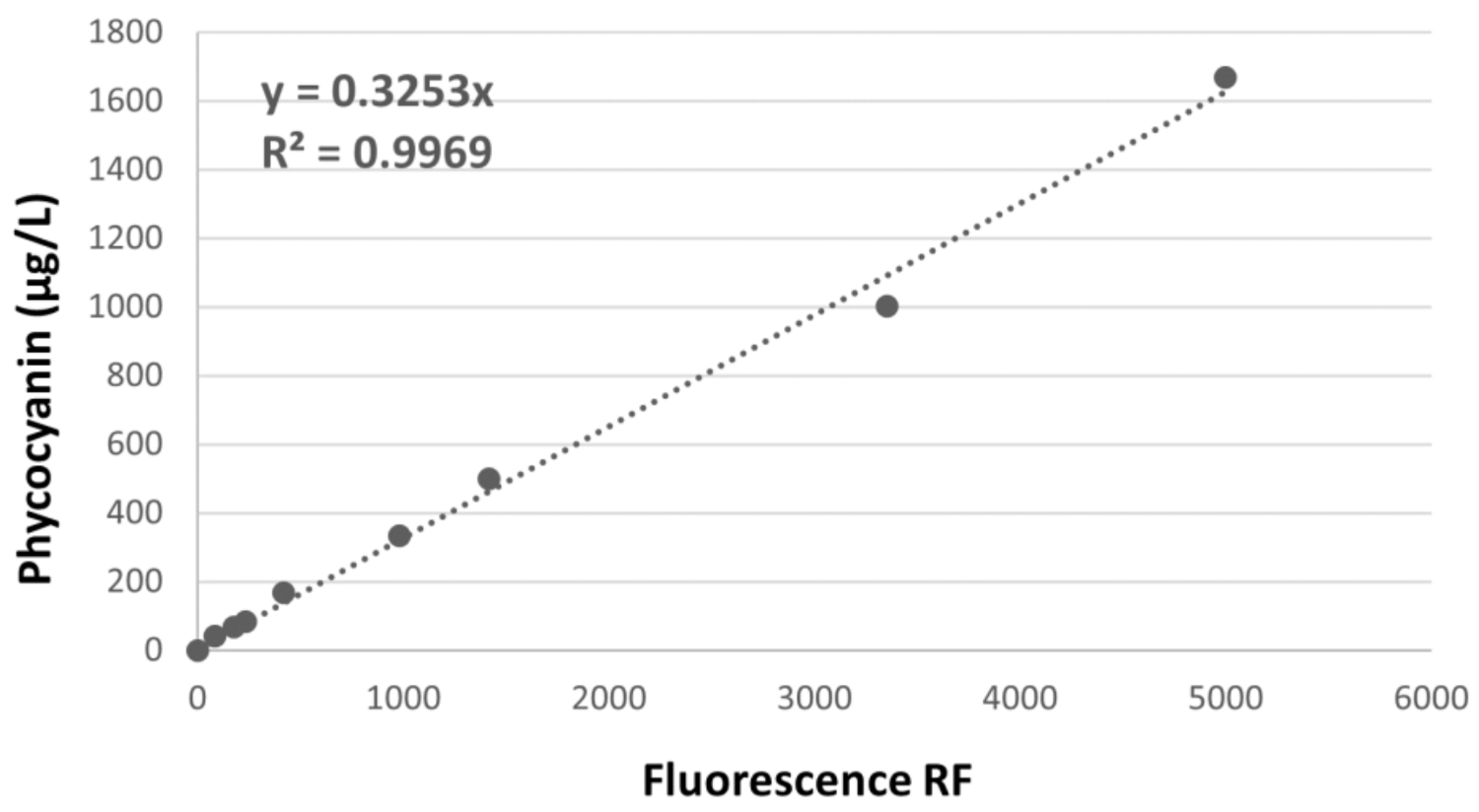
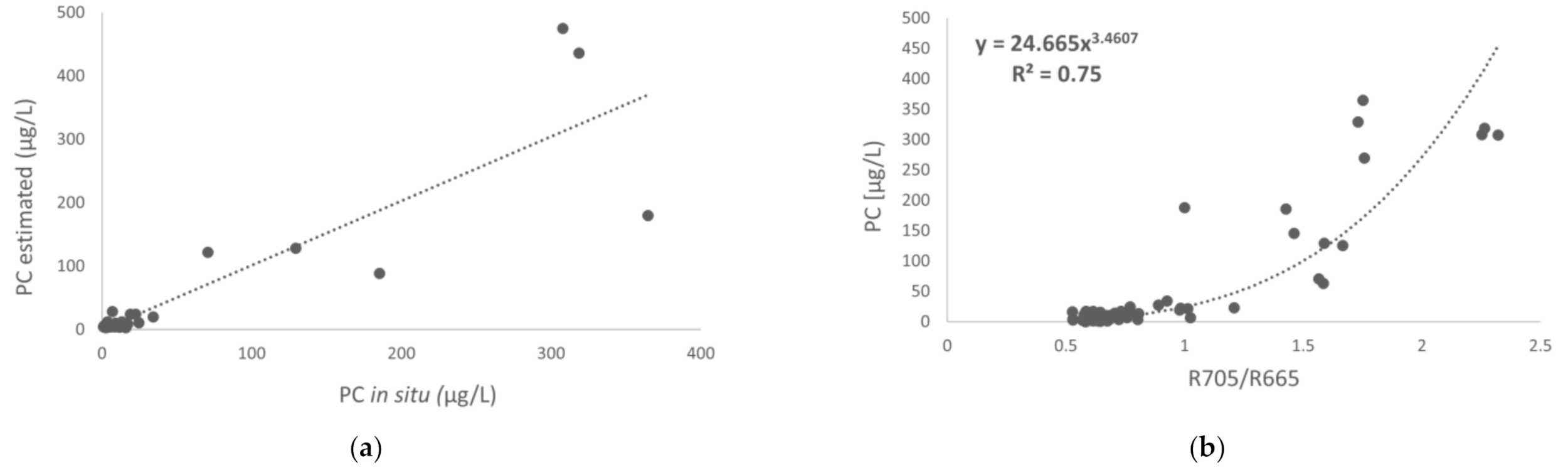
3.1. Calibration
3.2. Validation
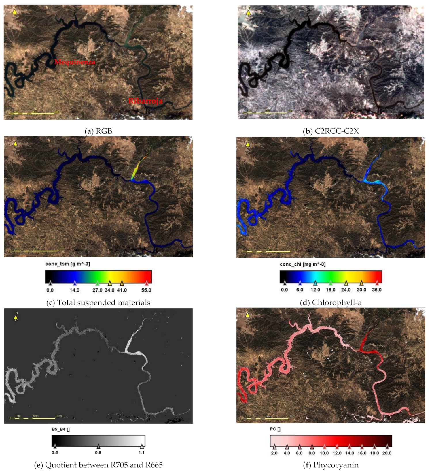
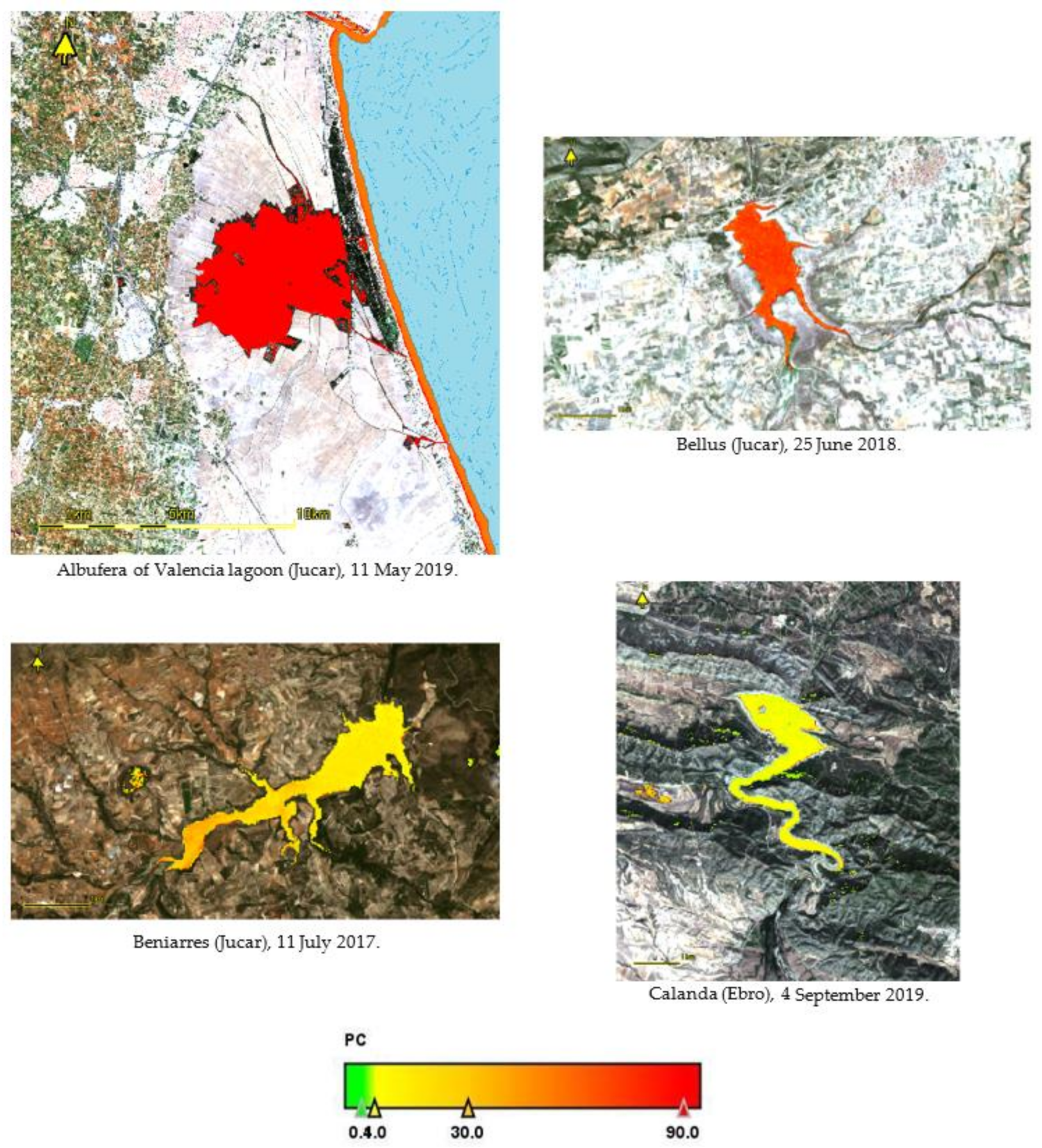
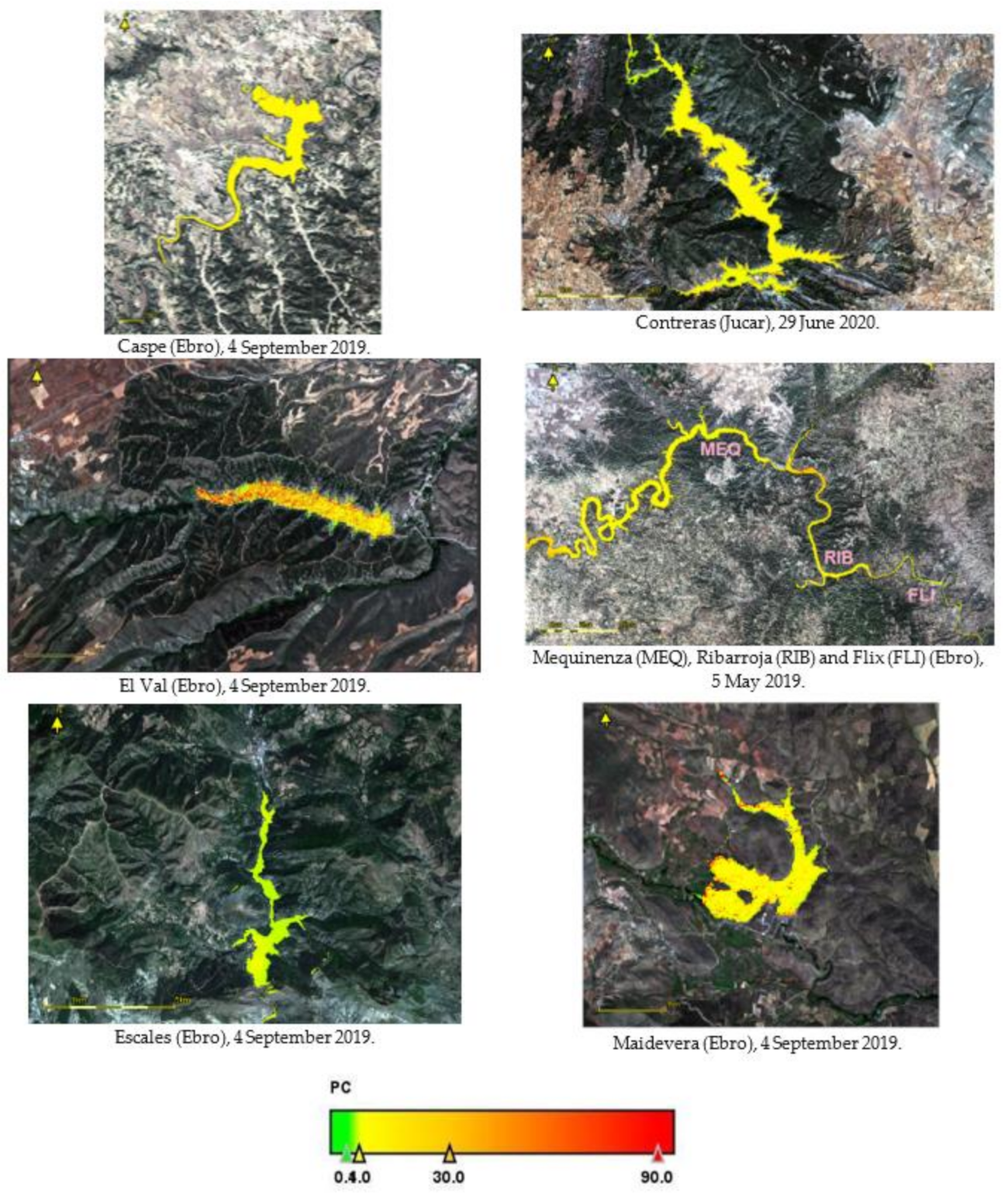
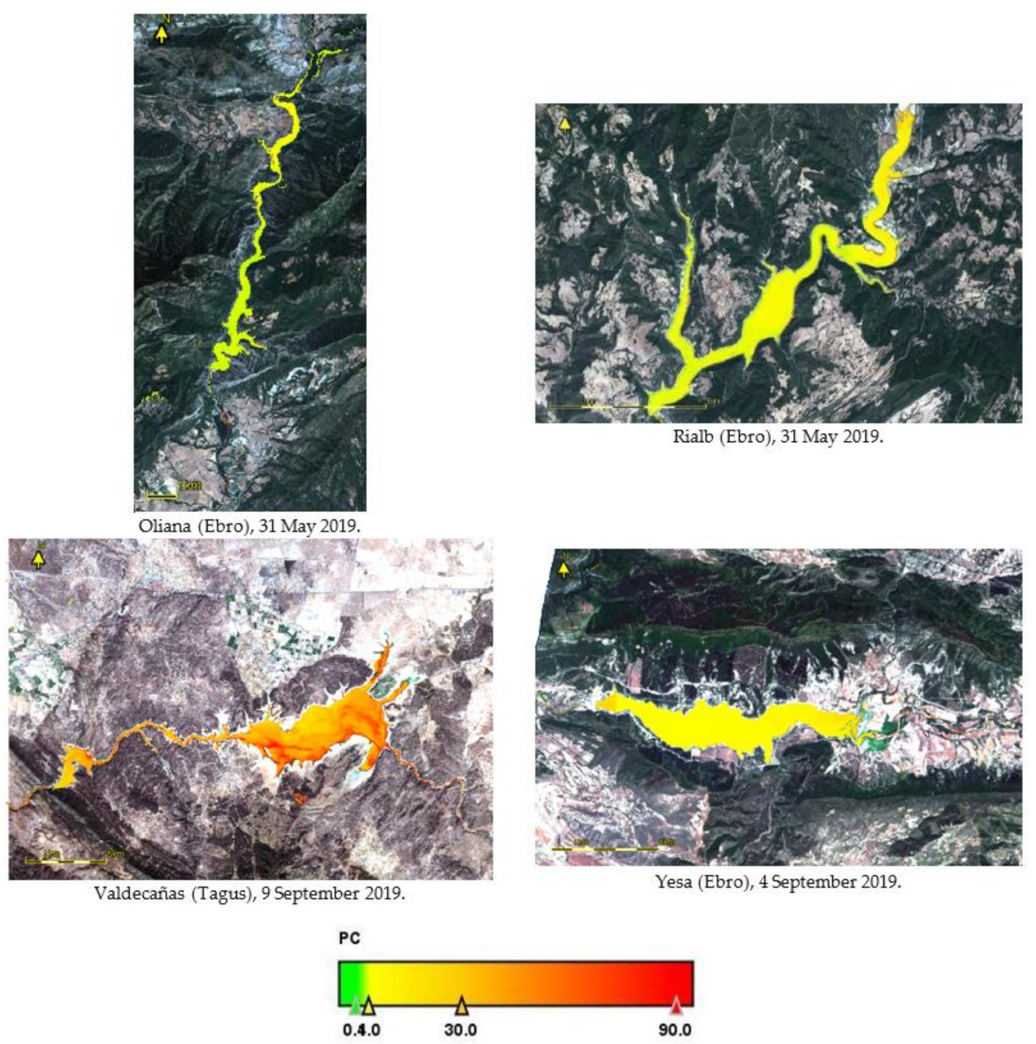
3.3. Thematic Maps
4. Discussion
4.1. Satellite Sensors and Spectral Resolution
4.2. Problems of Cyanobacteria
5. Conclusions
Author Contributions
Funding
Institutional Review Board Statement
Informed Consent Statement
Data Availability Statement
Acknowledgments
Conflicts of Interest
Appendix A

| Name | Position | Max Depth (m) | Volume (×106 m3) | Elevation (m.a.s.l.) | Res. Time (Year) | Climate | ||
|---|---|---|---|---|---|---|---|---|
| Lat. | Lon. | |||||||
| 1 | Alarcón | 39.69 | −2.17 | 71 | 1118 | 806 | 2.15 | Csa |
| 2 | Albufera | 39.34 | −0.35 | 2 | 23 | 1 | 0.15 | Csa |
| 3 | Barasona | 42.14 | 0.33 | 66 | 85 | 448 | 0.24 | Cfa |
| 4 | Bellus | 38.93 | −0.47 | 34 | 69 | 144 | 0.63 | Csa |
| 5 | Benageber | 39.73 | −1.09 | 90 | 221 | 450 | 0.35 | Csb |
| 6 | Beniarres | 38.80 | −0.35 | 53 | 27 | 318 | 1.22 | Csa |
| 7 | Canelles | 42.03 | 0.65 | 150 | 201 | 506 | 1.00 | Cfb |
| 8 | Contreras | 39.62 | −1.53 | 129 | 384 | 669 | 1.48 | Csa |
| 9 | Cueva Foradada | 40.97 | −0.69 | 65 | 22 | 580 | 0.65 | Bsk |
| 10 | Ebro | 42.97 | −4.07 | 34 | 540 | 838 | 1.55 | Cfb |
| 11 | Estanca de Alcañiz | 41.06 | −0.18 | 15 | 7 | 342 | 0.14 | BSk |
| 12 | Flix | 41.23 | 0.53 | 26 | 11 | 41 | 0.01 | BSk |
| 13 | Gallipuen | 40.87 | −0.41 | 36 | 4 | 694 | 0.71 | Cfb |
| 14 | La Loteta | 41.82 | −1.32 | 34 | 100 | 288 | 3.51 | BSk |
| 15 | Maria Cristina | 40.02 | −0.16 | 38 | 18 | 100 | 5.96 | Csa |
| 16 | Mezalocha | 41.42 | −1.07 | 45 | 4 | 473 | 1.17 | Cfa |
| 17 | Moneva | 41.17 | −0.83 | 45 | 8 | 615 | 0.95 | Cfb |
| 18 | Oliana | 42.12 | 1.30 | 102 | 84 | 519 | 0.08 | Cfa |
| 19 | Regajo | 39.89 | −0.52 | 23 | 6 | 407 | 0.14 | Csa |
| 20 | Rialb | 41.97 | 1.23 | 99 | 402 | 430 | 0.36 | Cfa |
| 21 | Ribarroja | 41.33 | 0.36 | 60 | 207 | 70 | 0.03 | Csb |
| 22 | Sitjar | 40.01 | −0.23 | 58 | 49 | 160 | 0.37 | Csa |
| 23 | Sobrón | 42.76 | −3.15 | 39 | 20 | 511 | 0.06 | Cfb |
| 24 | La Sotonera | 42.11 | −0.68 | 31 | 189 | 417 | 0.58 | Cfa |
| 25 | Terradets | 42.05 | 0.88 | 47 | 33 | 372 | 0.04 | Cfa |
| 26 | Tous | 39.13 | −0.65 | 110 | 378 | 135 | 0.28 | Csa |
| 27 | Tranquera | 41.24 | −1.78 | 81 | 84 | 684 | 0.68 | BSk |
| 28 | Urrunaga | 42.98 | −2.65 | 31 | 72 | 547 | 0.31 | Csb |
| 29 | Utchesa | 41.50 | 0.53 | 5 | 4 | 147 | 0.31 | BSk |
| 30 | Valdecañas | 39.82 | −5.42 | 98 | 1446 | 315 | 0.36 | Csb |
| Reservoir and Year | PC (μg/L) | Chl a (μg/L) | Reservoir and Year | PC (μg/L) | Chl a (μg/L) |
|---|---|---|---|---|---|
| Alarcon 2020 | 5.30 | 1.75 | Las Torcas 2017 | 2.98 | 1.72 |
| Alarcon 2020 | 5.60 | 1.80 | Lechago 2019 | 4.30 | 3.01 |
| Alarcon 2020 | 3.75 | 1.94 | Mansilla 2016 | 1.54 | 2.37 |
| Alarcon 2020 | 4.75 | 1.80 | Mansilla 2017 | 1.61 | 2.96 |
| Alarcon 2020 | 5.77 | 1.80 | Mezalocha 2017 | 34.08 | 7.65 |
| Alarcon 2020 | 5.97 | 1.10 | Mezalocha 2018 | 5.96 | 2.62 |
| Albufera 2020 | 188.14 | 30.14 | Moneva 2019 | 6.89 | 11.86 |
| Albufera 2020 | 269.55 | 81.34 | Monteagudo 2018 | 8.70 | 1.59 |
| Albufera 2020 | 329.05 | 91.92 | Oliana 2017 | 1.28 | 3.38 |
| Albufera 2020 | 364.70 | 90.93 | Oliana 2019 | 2.76 | 6.50 |
| Alloz 2017 | 3.10 | 1.34 | Oliana 2019 | 9.04 | 2.58 |
| Barasona 2018 | 2.57 | 1.67 | Regajo 2017 | 11.14 | 8.97 |
| Bellus 2017 | 185.43 | 61.39 | Regajo 2018 | 4.71 | 5.57 |
| Bellus 2018 | 307.93 | 49.09 | Regajo 2018 | 4.94 | 4.58 |
| Bellus 2018 | 318.50 | 51.59 | Regajo 2018 | 6.23 | 4.63 |
| Bellus 2018 | 307.72 | 41.54 | Rialb 2018 | 5.19 | 2.89 |
| Bellus 2020 | 63.15 | 24.59 | Rialb 2018 | 17.18 | 20.07 |
| Bellus 2020 | 70.67 | 25.83 | Rialb 2019 | 5.38 | 4.29 |
| Bellus 2020 | 129.52 | 30.06 | Ribarroja 2017 | 0.64 | 13.17 |
| Bellus 2021 | 125.61 | 29.95 | Santolea 2016 | 4.01 | 1.11 |
| Bellus 2021 | 145.27 | 29.87 | Sitjar 2017 | 3.49 | 0.61 |
| Benageber 2020 | 8.68 | 2.50 | Sitjar 2017 | 3.71 | 0.72 |
| Benageber 2017 | 9.06 | 5.77 | Sobron 2017 | 15.69 | 6.89 |
| Benageber 2017 | 10.53 | 5.47 | Sobron 2019 | 11.60 | 10.31 |
| Benageber 2018 | 8.01 | 4.91 | La Sotonera 2016 | 2.99 | 0.68 |
| Benageber 2018 | 7.26 | 4.85 | La Sotonera 2016 | 1.29 | 2.25 |
| Benageber 2018 | 8.19 | 4.91 | La Sotonera 2016 | 1.58 | 2.33 |
| Benageber 2020 | 7,05 | 2.12 | La Sotonera 2018 | 15.52 | 3.44 |
| Benageber 2020 | 8.80 | 2.44 | La Sotonera 2019 | 7.33 | 2.51 |
| Benageber 2020 | 10.53 | 2.96 | Terradets 2018 | 24.76 | 1.16 |
| Benageber 2020 | 7.37 | 2.38 | Tous 2017 | 1.70 | 1.85 |
| Benageber 2020 | 8.73 | 2.68 | Tous 2017 | 4.01 | 0.69 |
| Beniarres 2017 | 21.70 | 8.50 | Tous 2017 | 4.61 | 0.64 |
| Beniarres 2017 | 19.02 | 17.17 | Urrunaga 2018 | 16.79 | 3.21 |
| Canelles 2016 | 0.84 | 1.16 | Utchesa-Seca 2019 | 16.08 | 9.91 |
| Canelles 2016 | 1.62 | 2.86 | Valdecañas 2020 | 22.70 | 1.78 |
| Canelles 2020 | 1.93 | 1.41 | Valdecañas 2020 | 22.54 | 1.48 |
| Cazalegas 2020 | 230.98 | 6.93 | Yesa 2017 | 2.23 | 3.46 |
| Contreras 2018 | 8.37 | 2.46 | |||
| Cueva Foradada 2017 | 3.70 | 3.43 | |||
| Cueva Foradada 2018 | 13.23 | 14.22 | |||
| Ebro 2019 | 4.38 | 2.34 | |||
| Estanca de Alcañiz 2018 | 11.43 | 3.24 | |||
| Eugui 2017 | 2.93 | 5.95 | |||
| Flix 2018 | 14.29 | 2.28 | |||
| Galipuen 2019 | 27.28 | 3.41 | |||
| Itoiz 2017 | 2.36 | 2.52 | |||
| La Loteta 2019 | 9.10 | 1.83 | |||
| La Peña 2017 | 4.21 | 1.77 | |||
| La Tranquera 2016 | 10.94 | 5.95 | |||
| La Tranquera 2017 | 12.04 | 8.45 | |||
| La Tranquera 2018 | 17.35 | 11.75 |


References
- Soria, J.M.; Montagud, D.; Sòria-Perpinyà, X.; Sendra, M.D.; Vicente, E. Phytoplankton Reservoir Trophic Index (PRTI): A new tool for ecological quality studies. Inland Waters 2019, 9, 301–308. [Google Scholar] [CrossRef]
- Hallegraeff, G.; Anderson, D.M.; Hole, W.; Cembella, A. Harmful algal blooms: A global overview. In Manual on Harmful Marine Microalgae; UNESCO: Paris, France, 2003; Volume 33, pp. 1–22. [Google Scholar]
- World Health Organization (WHO). Guidelines for Drinking-Water Quality, 4th ed.; World Health Organization: Ginebra, Switzerland, 2011; p. 636. [Google Scholar]
- Lehner, B.; Döll, P.; Alcamo, J.; Henrichs, T.; Kaspar, F. Estimating the Impact of Global Change on Flood and Drought Risks in Europe: A Continental, Integrated Analysis. Clim. Chang. 2006, 75, 273–299. [Google Scholar] [CrossRef]
- European Commision. Water Framework Directive. Off. J. Ref. 2000, 327, 1–73. [Google Scholar]
- Castenholz, R.W. General characteristics of the cyanobacteria. In Bergey’s Manual of Systematics of Archaea and Bacteria; Wyley: Hoboken, NJ, USA, 2015; pp. 1–23. [Google Scholar] [CrossRef]
- Chorus, I.; Welker, M. (Eds.) Toxic Cyanobacteria in Water, 2nd ed.; CRC Press: Boca Raton, FL, USA; Geneva, Switzerland, 2021; p. 859. [Google Scholar]
- Huertas, I.E.; Rouco, M.; López-Rodas, V.; Costas, E. Warming will affect phytoplankton differently: Evidence through a mechanistic approach. Proc. R. Soc. B: Boil. Sci. 2011, 278, 3534–3543. [Google Scholar] [CrossRef] [PubMed] [Green Version]
- Whitton, B.A.; Potts, M. Introduction to the Cyanobacteria. In Ecology of Cyanobacteria II; Springer: Dordrecht, Germany, 2012; pp. 1–13. [Google Scholar]
- O’Neil, J.; Davis, T.; Burford, M.; Gobler, C. The rise of harmful cyanobacteria blooms: The potential roles of eutrophication and climate change. Harmful Algae 2012, 14, 313–334. [Google Scholar] [CrossRef]
- Kähler, P.; Koeve, W. Marine dissolved organic matter: Can its C:N ratio explain carbon overconsumption? Deep. Sea Res. Part I: Oceanogr. Res. Pap. 2001, 48, 49–62. [Google Scholar] [CrossRef]
- Hamilton, T.L.; Corman, J.R.; Havig, J.R. Carbon and nitrogen recycling during cyanoHABs in dreissenid-invaded and non-invaded US midwestern lakes and reservoirs. Hydrobiologia 2019, 847, 939–965. [Google Scholar] [CrossRef] [Green Version]
- Carmichael, W.W. The Toxins of Cyanobacteria. Sci. Am. 1994, 270, 78–86. [Google Scholar] [CrossRef]
- Randolph, K.; Wilson, J.; Tedesco, L.; Li, L.; Pascual, D.L.; Soyeux, E. Hyperspectral remote sensing of cyanobacteria in turbid productive water using optically active pigments, chlorophyll a and phycocyanin. Remote. Sens. Environ. 2008, 112, 4009–4019. [Google Scholar] [CrossRef]
- Zanchett, G.; Oliveira-Filho, E.C. Cyanobacteria and Cyanotoxins: From Impacts on Aquatic Ecosystems and Human Health to Anticarcinogenic Effects. Toxins 2013, 5, 1896–1917. [Google Scholar] [CrossRef]
- Glazer, A.N. Light guides. Directional energy transfer in a photosynthetic antenna. J. Biol. Chem. 1989, 264, 1–4. [Google Scholar] [CrossRef]
- Glazer, A.N. Phycobilisome a macromolecular complex optimized for light energy transfer. Biochim. Biophys. Acta Rev. Bioenerg. 1984, 768, 29–51. [Google Scholar] [CrossRef]
- Brient, L.; Lengronne, M.; Bertrand, E.; Rolland, D.; Sipel, A.; Steinmann, D.; Baudin, I.; Legeas, M.; Le Rouzic, B.; Bormans, M. A phycocyanin probe as a tool for monitoring cyanobacteria in freshwater bodies. J. Environ. Monit. 2008, 10, 248–255. [Google Scholar] [CrossRef]
- Damar, A.; Colijn, F.; Hesse, K.-J.; Kurniawan, F. Coastal Phytoplankton Pigments Composition in Three Tropical Estuaries of Indonesia. J. Mar. Sci. Eng. 2020, 8, 311. [Google Scholar] [CrossRef]
- Gomarasca, M.A.; Giardino, C.; Bresciani, M.; De Carolis, G.; Sandu, C.; Tornato, A.; Tonolo, F. Copernicus Sentinel missions for water resources. In Proceedings of the 6th International Conference on Space Science and Communication, Kebangsaan, Malaysia, 28-30 June 2019. [Google Scholar]
- European Space Agency (ESA). Sentinel-2 Spectral Response Functions. 2017. Available online: https://sentinel.esa.int/web/sentinel/user-guides/sentinel-2-msi/document-library/-/asset_publisher/Wk0TKajiISaR/content/sentinel-2a-spectral-responses (accessed on 10 June 2021).
- Shoaf, W.T.; Lium, B.W. Improved extraction of chlorophyll a and b from algae using dimethyl sulfoxide. Limnol. Oceanogr. 1976, 21, 926–928. [Google Scholar] [CrossRef]
- Jeffrey, S.T.; Humphrey, G.F. New spectrophotometric equations for determining chlorophylls a, b, c1 and c2 in higher plants, algae and natural phytoplankton. Biochem. Physiol. Pflanz. 1975, 167, 191–194. [Google Scholar] [CrossRef]
- Radin, C.; Sòria-Perpinyà, X.; Delegido, J. Multitemporal water quality study in Sitjar (Castelló, Spain) reservoir using Sentinel-2 images. Rev. Teledetec. 2020, 56, 117–130. [Google Scholar] [CrossRef]
- Toming, K.; Kutser, T.; Laas, A.; Sepp, M.; Paavel, B.; Nõges, T. First Experiences in Mapping Lake Water Quality Parameters with Sentinel-2 MSI Imagery. Remote. Sens. 2016, 8, 640. [Google Scholar] [CrossRef] [Green Version]
- Beck, R.; Xu, M.; Zhan, S.; Liu, H.; Johansen, R.A.; Tong, S.; Yang, B.; Shu, S.; Wu, Q.; Wang, S.; et al. Comparison of Satellite Reflectance Algorithms for Estimating Phycocyanin Values and Cyanobacterial Total Biovolume in a Temperate Reservoir Using Coincident Hyperspectral Aircraft Imagery and Dense Coincident Surface Observations. Remote Sens. 2017, 9, 538. [Google Scholar] [CrossRef] [Green Version]
- Sòria-Perpinyà, X.; Vicente, E.; Urrego, P.; Pereira-Sandoval, M.; Ruíz-Verdú, A.; Delegido, J.; Soria, J.; Moreno, J. Remote sensing of cyanobacterial blooms in a hypertrophic lagoon (Albufera of València, Eastern Iberian Peninsula) using multitemporal Sentinel-2 images. Sci. Total Environ. 2020, 698, 134305. [Google Scholar] [CrossRef]
- Kwon, Y.S.; Pyo, J.; Duan, H.; Cho, K.H.; Park, Y. Drone-based hyperspectral remote sensing of cyanobacteria using vertical cumulative pigment concentration in a deep reservoir. Remote Sens. Environ. 2020, 236, 111517. [Google Scholar] [CrossRef]
- Liu, G.; Simis, S.G.H.; Li, L.; Wang, Q.; Li, Y.; Song, K.; Lyu, H.; Zheng, Z.; Shi, K. A Four-Band Semi-Analytical Model for Estimating Phycocyanin in Inland Waters From Simulated MERIS and OLCI Data. IEEE Trans. Geosci. Remote Sens. 2017, 56, 1374–1385. [Google Scholar] [CrossRef]
- Chorus, I.; Bartram, J. Toxic Cyanobacteria in Water. A Guide to their Public Health Consequences, Monitoring and Management; E&FN Spon on behalf of the World Health Organization; Chorus, I., Welker, M., Eds.; CRC Press: London, UK, 1999; pp. 1–416. [Google Scholar] [CrossRef]
- Ruiz-Verdú, A.; Simis, S.; de Hoyos, C.; Gons, H.J.; Peña-Martínez, R. An evaluation of algorithms for the remote sensing of cyanobacterial biomass. Remote Sens. Environ. 2008, 112, 3996–4008. [Google Scholar] [CrossRef]
- Sòria-Perpinyà, X.; Vicente, E.; Urrego, P.; Pereira-Sandoval, M.; Tenjo, C.; Ruíz-Verdú, A.; Delegido, J.; Soria, J.; Peña, R.; Moreno, J. Validation of Water Quality Monitoring Algorithms for Sentinel-2 and Sentinel-3 in Mediterranean Inland Waters with In Situ Reflectance Data. Water 2021, 13, 686. [Google Scholar] [CrossRef]
- Viso-Vázquez, M.; Acuña-Alonso, C.; Rodríguez, J.; Álvarez, X. Remote Detection of Cyanobacterial Blooms and Chlorophyll-a Analysis in a Eutrophic Reservoir Using Sentinel-2. Sustainability 2021, 13, 8570. [Google Scholar] [CrossRef]
- Paerl, H.W.; Xu, H.; McCarthy, M.J.; Zhu, G.; Qin, B.; Li, Y.; Gardner, W.S. Controlling harmful cyanobacterial blooms in a hyper-eutrophic lake (Lake Taihu, China): The need for a dual nutrient (N & P) management strategy. Water Res. 2011, 45, 1973–1983. [Google Scholar] [CrossRef]
- Kühl, M.; Fenchel, T. Bio-optical Characteristics and the Vertical Distribution of Photosynthetic Pigments and Photosynthesis in an Artificial Cyanobacterial Mat. Microb. Ecol. 2000, 40, 94–103. [Google Scholar] [CrossRef] [PubMed]
- Hoyos, C.D.; Negro, A.I.; Aldasoro-Martín, J.J. Cyanobacteria distribution and abundance in the Spanish water reservoirs during thermal stratification. Limnetica 2004, 23, 119–132. [Google Scholar]
- Navarro, E.; Caputo, L.; Marcé, R.; Carol, J.; Benejam, L.; García-Berthou, E.; Armengol, J. Ecological classification of a set of Mediterranean reservoirs applying the EU Water Framework Directive: A reasonable compromise between science and management. Lake Reserv. Manag. 2009, 25, 364–376. [Google Scholar] [CrossRef] [Green Version]
- Durall, C.; Lindblad, P. Mechanisms of carbon fixation and engineering for increased carbon fixation in cyanobacteria. Algal Res. 2015, 11, 263–270. [Google Scholar] [CrossRef]
- Izydorczyk, K.; Tarczynska, M.; Jurczak, T.; Mrowczynski, J.; Zalewski, M. Measurement of phycocyanin fluorescenceas an online early warning system for cyanobacteria in reservoir intake water. Environ. Toxicol. 2005, 20, 425–430. [Google Scholar] [CrossRef]
- Ahn, C.-Y.; Joung, S.-H.; Yoon, S.-K.; Oh, H.-M. Alternative alert system for cyanobacterial bloom, using phycocyanin as a level determinant. J. Microbiol. 2007, 45, 98–104. [Google Scholar]
- Li, L.; Sengpiel, R.E.; Pascual, D.L.; Tedesco, L.P.; Wilson, J.S.; Soyeux, E. Using hyperspectral remote sensing to estimate chlorophyll-a and phycocyanin in a mesotrophic reservoir. Int. J. Remote Sens. 2010, 31, 4147–4162. [Google Scholar] [CrossRef]
- Ogashawara, I. The Use of Sentinel-3 Imagery to Monitor Cyanobacterial Blooms. Environments 2019, 6, 60. [Google Scholar] [CrossRef] [Green Version]


| Band | Wavelength (nm) | Spatial Resolution (m) | Objective | ||
|---|---|---|---|---|---|
| Central | Wide | ||||
| B1 | VIS | 443 | 20 | 60 | Aerosol Correction |
| B2 | 490 | 65 | 10 | Aerosol Correction, Blue Band Measure | |
| B3 | 560 | 35 | 10 | Green Band Measure | |
| B4 | 665 | 30 | 10 | Red Band Measure | |
| B5 | NIR | 705 | 15 | 20 | Red Edge 1 Band Measure |
| B6 | 740 | 15 | 20 | Red Edge 2 Band Measure | |
| B7 | 783 | 20 | 20 | Red Edge 3 Band Measure | |
| B8 | 842 | 115 | 10 | Water Vapor Correction, Near Infrared Band | |
| B8a | 865 | 20 | 20 | Water Vapor Correction, Near Infrared Band | |
| B9 | 945 | 20 | 60 | Water Vapor Correction, Near Infrared Band | |
| B10 | SWIR | 1380 | 20 | 60 | Cirrus Detection, Infrared Band |
| B11 | 1610 | 90 | 20 | Infrared Band | |
| B12 | 2190 | 180 | 20 | Aerosol Correction, Infrared Band | |
| Reference | Sensor | Atmospheric Correction | Bands Relation | N | R2 | RMSE | Data Range |
|---|---|---|---|---|---|---|---|
| [25] | S2-MSI | In situ Reflectance | R740−R665 | 29 | 0.70 | 4.82 | 0–23 RFU |
| [25] | S3-OLCI | In situ Reflectance | R707/R679 | 9 | 0.86 | 1.45 | 0–23 RFU |
| [26] | S2-MSI | Sen2cor | R740/R665 | 21 | 0.84 | 141 | 10–1287 mg/m3 |
| [27] | Dron | - | R709/R620 | 92 | 0.95 | - | 0.43–13.07 mg/m3 |
| [28] | S3-OLCI | In situ Reflectance | 216 | 0.69 | 22.7 | 0.33–317.74 mg/m3 | |
| This Study | S2-MSI | C2X | R705−R665 | 45 | - | - | 0.23–364.7 mg/m3 |
| Drinking Water | Bath Water | Density (Cell mL−1) | Biovolum (mm3 L−1) | Chlorophylla (µg L−1) | PC (µg L−1) |
|---|---|---|---|---|---|
| Surveillance level | 200 | 0.02 | 0.1 | <0.1 | |
| Alert level I | 2000 | 0.2 | 1.0 | 4 | |
| Guidance level I | 20,000 | 2 | 10 | 30 ± 2 | |
| Alert level II | Guidance level II | 100,000 | 10 | 50 | 90 ± 2 |
| Chl-a (μg L−1) | SDD (m) | SS (mg L−1) | PC (µg L−1) | |
|---|---|---|---|---|
| Maximum | 91.92 | 9.10 | 48.56 | 364.70 |
| Minimum | 0.61 | 0.35 | 0.30 | 0.23 |
| Mean | 9.82 | 3.36 | 6.07 | 37.56 |
| St. Deviation | 16.61 | 2.23 | 10.77 | 80.18 |
| Band Ratio | PC | R2 | PC Log. | R2 |
|---|---|---|---|---|
| [25] | −295.15 (R740 − R665) + 36.165 | 0.0007 | 0.05 | |
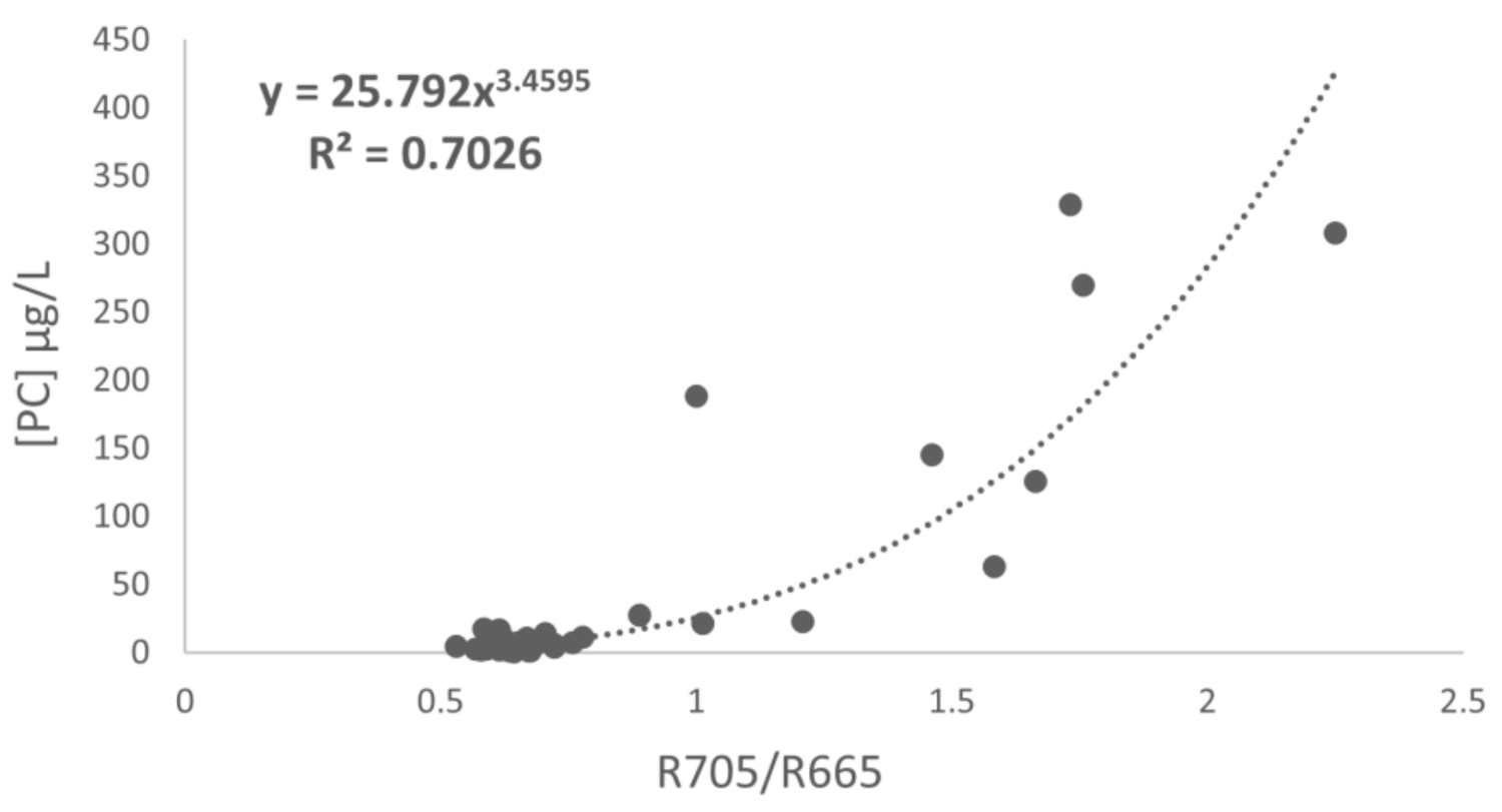
| [25,27] | 25.792 (R705/R665)3.4595 | 0.70 | 0.69 | |
| [26] | 387.84 (R740/R665)2.3932 | 0.67 | 0.64 | |
| [28] | 0.74 | 0.59 | ||
| R705−R665 | 0.64 | 0.51 |
| Band Ratio | Equation | R2 | RMSE (µg L−1) | RRMSE (%) |
|---|---|---|---|---|
| R740 − R665 | y = −47.348 x + 1.9091 | 0.02 | 13.42 | 31.22 |
| R740/R665 | y = 387.84 x2.3932 | 0.61 | 9.92 | 23.08 |
| R705/R665 | y = 24.665 x3.4607 | 0.71 | 8.13 | 18.91 |
| R705 − R665 | y = 8595.3 x + 38.796 | 0.72 | 7.21 | 16.78 |
| y = 669.65 x +14.808 | 0.66 | 7.82 | 18.19 |
Publisher’s Note: MDPI stays neutral with regard to jurisdictional claims in published maps and institutional affiliations. |
© 2021 by the authors. Licensee MDPI, Basel, Switzerland. This article is an open access article distributed under the terms and conditions of the Creative Commons Attribution (CC BY) license (https://creativecommons.org/licenses/by/4.0/).
Share and Cite
Pérez-González, R.; Sòria-Perpinyà, X.; Soria, J.M.; Delegido, J.; Urrego, P.; Sendra, M.D.; Ruíz-Verdú, A.; Vicente, E.; Moreno, J. Phycocyanin Monitoring in Some Spanish Water Bodies with Sentinel-2 Imagery. Water 2021, 13, 2866. https://doi.org/10.3390/w13202866
Pérez-González R, Sòria-Perpinyà X, Soria JM, Delegido J, Urrego P, Sendra MD, Ruíz-Verdú A, Vicente E, Moreno J. Phycocyanin Monitoring in Some Spanish Water Bodies with Sentinel-2 Imagery. Water. 2021; 13(20):2866. https://doi.org/10.3390/w13202866
Chicago/Turabian StylePérez-González, Rebeca, Xavier Sòria-Perpinyà, Juan Miguel Soria, Jesús Delegido, Patricia Urrego, María D. Sendra, Antonio Ruíz-Verdú, Eduardo Vicente, and José Moreno. 2021. "Phycocyanin Monitoring in Some Spanish Water Bodies with Sentinel-2 Imagery" Water 13, no. 20: 2866. https://doi.org/10.3390/w13202866
APA StylePérez-González, R., Sòria-Perpinyà, X., Soria, J. M., Delegido, J., Urrego, P., Sendra, M. D., Ruíz-Verdú, A., Vicente, E., & Moreno, J. (2021). Phycocyanin Monitoring in Some Spanish Water Bodies with Sentinel-2 Imagery. Water, 13(20), 2866. https://doi.org/10.3390/w13202866