Article

Characterization of the Transpiration of a Vineyard under Different Irrigation Strategies Using Sap Flow Sensors

by
Luis Alberto Mancha
*,
David Uriarte
and
María del Henar Prieto
Center for Scientific and Technological Research of Extremadura (CICYTEX), Agricultural Research Institute “Finca La Orden-Valdesequera”, Highway A-5 km. 372, Guadajira, 06187 Badajoz, Spain
*
Author to whom correspondence should be addressed.
Water 2021, 13(20), 2867; https://doi.org/10.3390/w13202867
Submission received: 21 September 2021 / Revised: 5 October 2021 / Accepted: 12 October 2021 / Published: 14 October 2021

Abstract

:
Lysimeters are the reference method for determining ETc, but they are expensive and complex, which limits their use. The first objective of this work was to adjust and evaluate the robustness of sap flow sensors in order to determine the transpiration of a vineyard and, together with an evaporation model, to calculate the ETc of the vineyard. For this purpose, we compared water consumption data obtained from a vineyard weighing lysimeter (ETcLys) with the sum of transpiration obtained from sap flow sensors (TSF) and evaporation estimated empirically over four years (2012, 2013, 2014 and 2015). The second objective was to obtain the relationship between the vegetative growth and transpiration of the vines with different water availability (irrigation and rainfed treatments), as an alternative method for estimating vine water needs adjusted to their real development. The third and last objective was to evaluate the transpiration response of the vines when subjected to water stress. We carried out the work in an experimental vineyard which has a well-established weighing lysimeter. As a result, a good match was obtained between vine sap flow and transpiration (R2 = 0.85) as well as a good relationship between vegetative growth and vine transpiration (FiPAR: R2Irrigation = 0.34. R2Rainfed = 0.54; LAI: R2Irrigation = 0.68. R2Rainfed = 0.53).

1. Introduction

The quantification of vineyard water needs constitutes a critical step in the adoption of successful irrigation strategies. Irrigation management is the major and most controllable determinant of grape quality in arid areas [1]. Introducing the water needs of the crop into a water balance allows the volume of irrigation water to be adjusted to the crop requirements [2]. For practical purposes, crop water needs are assimilated to the ETc, which includes both plant transpiration and soil evaporation. They are obtained under standard conditions, corresponding to a disease-free and well-fertilized crop growing in a large field with optimal water content and reaching the maximum production for these agro-climatic conditions [3,4]. ETc has an important seasonal (from budbreak to leaf fall) and interannual variation, as it changes according to weather conditions, cropping practices and irrigation scheduling and strategy [3,5,6,7]. However, both soil and climate are determinants of the agronomic behavior of grapevines [8], known as the terroir effect [9], and to which varietal aspects must be added.
Among the methods used in the determination of ETc, the use of weighing lysimeters is the most direct methodology [10] and the one that offers the highest accuracy and time resolution [11]. It is considered the main reference method for the adjustment of other methodologies. There are very few weighing lysimeters for the study of grapevine; two of them are in Spain and one of these [6] was used in this study. This infrastructure is expensive and immovable. These limitations make it difficult to evaluate the influence that different agroecological aspects can have on vineyard water consumption with this system. However, other methods for determining ETc which, although a priori may be more imprecise, are more affordable and versatile. Among these are the water balance, widely used in woody crops. [12,13,14,15,16], Bowen ratio techniques [17,18], which are based on the eddy correlation [19,20,21] and the surface renewal method [22]. Another possible approach is to calculate or measure the two components of ETc separately [23].
Several techniques are currently available to measure or estimate water use in woody plants. Those that use basic measurements of water movement through the plant are based on the properties of heat dissipation through the flow of sap through the stem [24] and offer several advantages: direct measurement of water through the plant (or smaller sections of the pathway); continuous, long-term monitoring without interruption of the plant canopy or root environment; and automation of transpiration rate calculation. The three types available are: heat dissipation, heat balance, and heat pulse [23,25,26]. The sap flow methods allow estimation of water losses in the plant by transpiration (T), measuring the speed at which the sap flow moves through the xylem. Discontinuous heat pulse methods are the most suitable for monitoring water in the tree under field conditions since they have lower energy requirements [27]. Of the latter, the heat pulse compensation method is the most appropriate for low and moderate flows [28], being a reliable technique for the continuous measurement of sap velocity in woody crops [27,29,30,31,32]. Some authors have suggested that sap flow measurement can be helpful for irrigation management in vineyards [19,33,34,35], although there is some uncertainty given the different approaches used as to the accuracy with which actual plant water consumption is determined. In these cases, it is recommended to perform direct calibrations which, in field conditions, can be performed with lysimeters [24,36], with the log cutting method [30], with gas exchange measurement chambers in complete plants [37,38,39], with a water balance under conditions in which evaporation is eliminated or quantified separately, or with micrometeorological methods [40].
Another important application of sap flow measurements is to gain insight into the dynamics of transpiration in the plant [23,41], especially in deficit irrigation studies where the objective is to quantify the reduction in net transpiration related to the water stress endured by the plants [42].
Soil evaporation (E) can be a quantitatively important component of crop water requirements, varying substantially depending on the frequency and method of irrigation, the soil maintenance system, and crop cover. Therefore, determining it independently of T is of interest when proposing more efficient systems of water use by crops [43]. In this sense, the UN’s Food and Agriculture Organization (FAO) presents a dual crop coefficient approach, in which the effects of T and E on ETc are determined separately using two coefficients: the basal crop coefficient (Kcb) to describe T and the evaporation coefficient (Ke) to describe E [3]. Different methodologies can be used to quantify E: empirical measurements or adapted models [44,45], using microlysimeters [46] or by covering cycles in a weighing lysimeter [5].
In most Spanish and worldwide wine-growing areas, irrigation is a crucial element to improve the water status of the vines, impacting on productivity and the characteristics of the grapes. The effect of environment on water status through stomatal conductance has been well interpreted in this species [47,48], as well as leaf water potential [49,50,51], stem water potential [52] and transpiration under water stress conditions [48].
Vegetative growth is one of the physiological processes most sensitive to water deficit in plants [53,54]. The increase in water available to the vineyard is usually accompanied by greater vigor, more vegetative development, and a higher leaf area [55]. A close relationship has been obtained between the water consumption and vegetative development of Tempranillo vines [6], as well as for cv. Thomson Seedless [7]. Relationships of this type have also been determined with the leaf area index (LAI) for clementines [56], and apple and pear trees [57], and with the radiation interception fraction for peach [2] and orange trees [58].
Although several studies have been published on the determination of vine water requirements using different methodologies [6,18,19,20,35,59], few studies have separated the two components of vineyard ETc (E and T). The first objective of this study was to adjust and evaluate sap flow sensors with the help of a weighing lysimeter, determine vineyard transpiration and then, together with an evaporation model, the ETc. The second objective was to determine the relationship between vegetative development and T of the vines with different water availability (irrigated and dry) as an alternative method for the evaluation of water consumption and, finally, to evaluate the effect of water stress on vine transpiration.

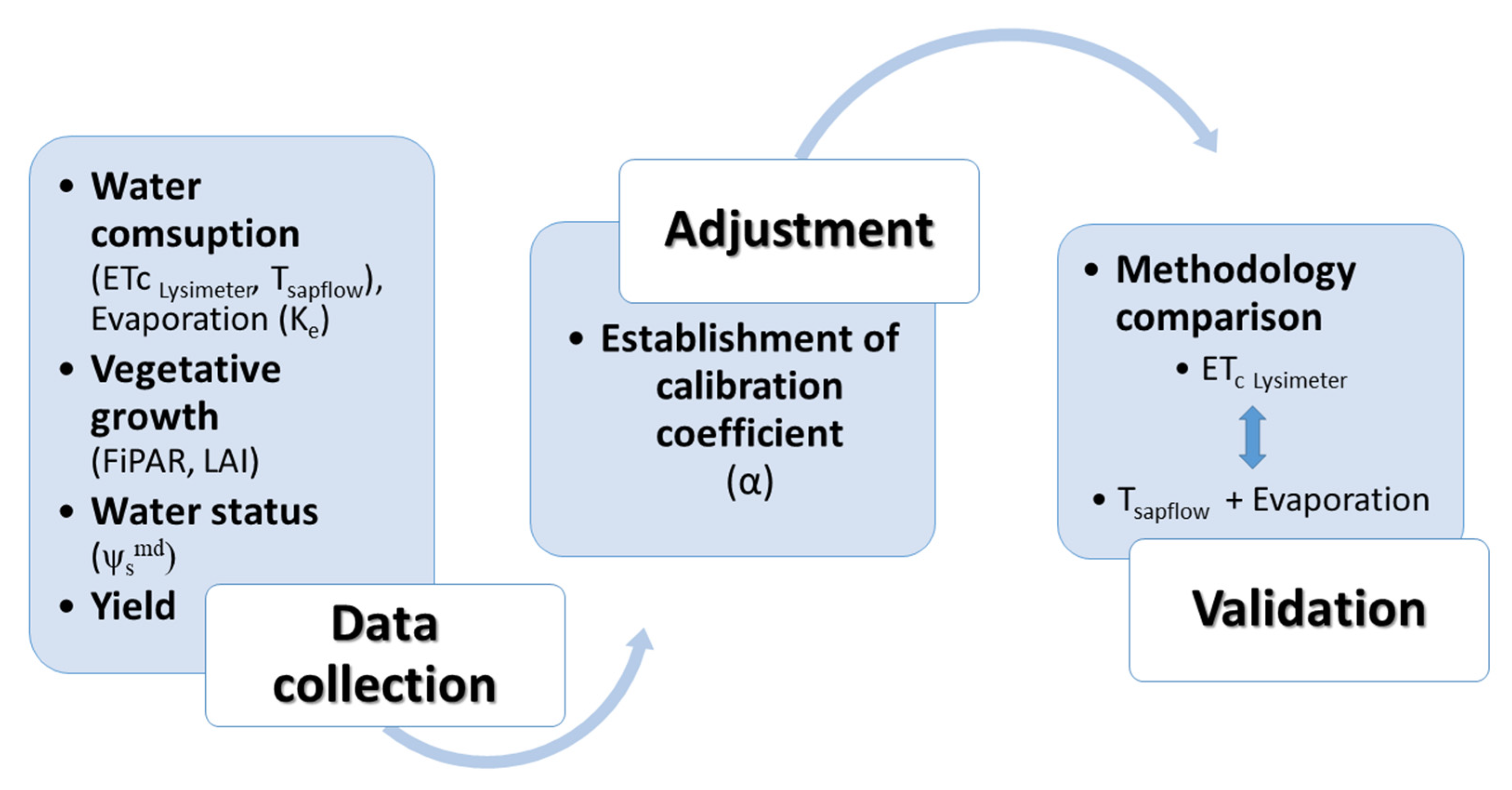
2. Materials and Methods

2.1. Location, Description of the Vineyard, and Weather Conditions

The trial was carried out during the 2012, 2013, 2014, and 2015 agricultural seasons in an experimental cv. Tempranillo vineyard of 1.7 ha located at “Finca La Orden” in Badajoz (38°51′ N, 6°40′ W, altitude 188 m), Spain. Planted in 2001, the vine was grafted on Richter 110 rootstock, trained on a trellis and formed in a double Royat cordon, leaving six spurs per plant and two buds per spur. The planting frame is 2.5 × 1.2 m, with a trunk height of 0.60 m and a trellis height of 1.50 m, in an east-west row orientation. In addition to winter pruning, the number of shoots per vine was adjusted in the spring (12 shoots per vine). We also carried out a clipping to contain the vegetation on the trellis.
The soil is alluvial, with a loam to sandy loam texture, slightly acidic, and lacking in organic matter. Soil depth is greater than 2.5 m and with low stone content. The area has a Mediterranean climate with a mild Atlantic influence, dry and hot summers, with high daily radiation and evaporative demand. We obtained agrometeorological data from a station close to the vineyard (100 m) with the characteristics described in [60]. We calculated the vapor pressure deficit (VPD) with the maximum and minimum temperatures and relative humidity [3].

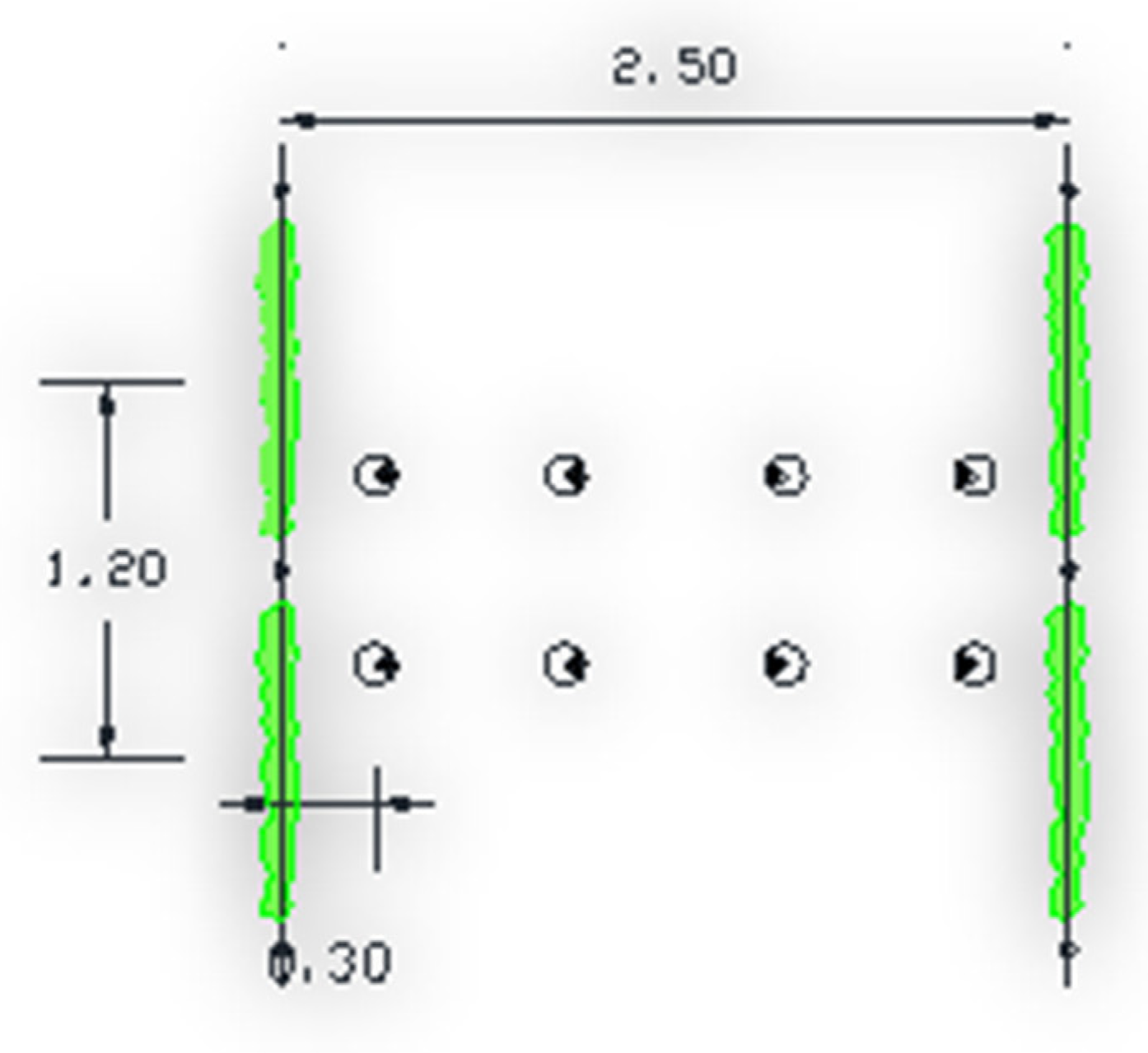
2.2. Experimental Design

In the experimental vineyard, we established two treatments (Irrigated and Rainfed) with a randomized block design with four replications per treatment. Each experimental plot consisted of 6 rows with 18 vines each row (108 plants per experimental plot), with the two outer rows as borders, and the four remaining rows under study. The lysimeter is located in the irrigation plot of block III, in a central position in the vineyard. In this block, we selected four vines per treatment for the installation of sap flow sensors, with two of these being the vines of the weighing lysimeter.

2.3. Irrigation Scheduling

The vines were irrigated daily with a drip irrigation system with two self-compensating emitters per vine (4 l h−1 for each dripper). Irrigation started when plants reached a midday stem water potential (Ψsmd) threshold value of −0.6 MPa in order to avoid water stress situations [61,62], and was maintained until the first half of October. At each irrigation, we applied a volume of water equal to the water consumed (100% ETc), quantified with a weighing lysimeter, since the previous irrigation. The size of the weighing lysimeter was 2.67 × 2.25 m and 1.5 m deep. A detailed description of the weighing lysimeter can be found in [6]. We obtained the reference evapotranspiration (ETo) from an agrometeorological station located 100 m from the experimental vineyard and run by the Irrigation Advisory Network of Extremadura (Spanish initials REDAREX; www.redarexplus.gobex.es/RedarexPlus, (daily access each year of study from April 1 to October 31) (accessed on 3 October 2021)), using the FAO-56 Penman-Monteith method [3].

2.4. Vegetative Growth, Water Status and Production

We characterized vegetative growth by determining the fraction of intercepted photosynthetically active radiation (FiPAR) and LAI. FiPAR, from two labelled vines per elementary plot, was measured at noon with a linear ceptometer (80 cm probe length; Accupar Linear PAR LP-80; Decagon Devices, Pullman, WA, USA). Measurements were taken every two weeks at solar noon on clear days from flowering to the onset of senescence, following the methodology described in [63]. We obtained FiPAR values in rainfed areas for 2012 and 2013 from the empirical relationship between LAI and FiPAR obtained during the four years under study, using the following linear equation:
(LAI = 9.1197 FiPAR − 0.0392; R2 = 0.75; n = 32)
LAI was measured periodically along the crop cycle every year, except in 2015 when only two measurements were made, with an LAI-2200 canopy analyzer (Li-Cor Inc. Lincoln, NE, USA). A baseline measurement was taken above the vegetation, followed immediately by measuring eight points at ground level in the center of eight quadrants into which the planting frame had been divided (Scheme 1). We used the LAI measurements obtained to determine the leaf area (LA) of the vine, using a previously established empirical relationship in the same experimental vineyard [64]:
(LA = 3.1076 LAI + 0.0198; R2 = 0.96)
We measured the Ψsmd on leaves placed at least 2 h previously in plasticized and aluminum-coated bags, from the north side and the lower part of the canopy close to the cordon [65]. Measurements were made with a Scholander pressure chamber (Soil Moisture Corp., Model 3500, Santa Barbara, CA, USA) on two leaves per experimental plot (1 per vine) at weekly intervals.
Harvesting was performed in each plot when the concentration of soluble solids was close to 23 °Brix (mean value of each treatment). We weighed and counted all the bunches of 10 previously selected plants from each experimental plot at harvest time, determining the average yield for each plot.

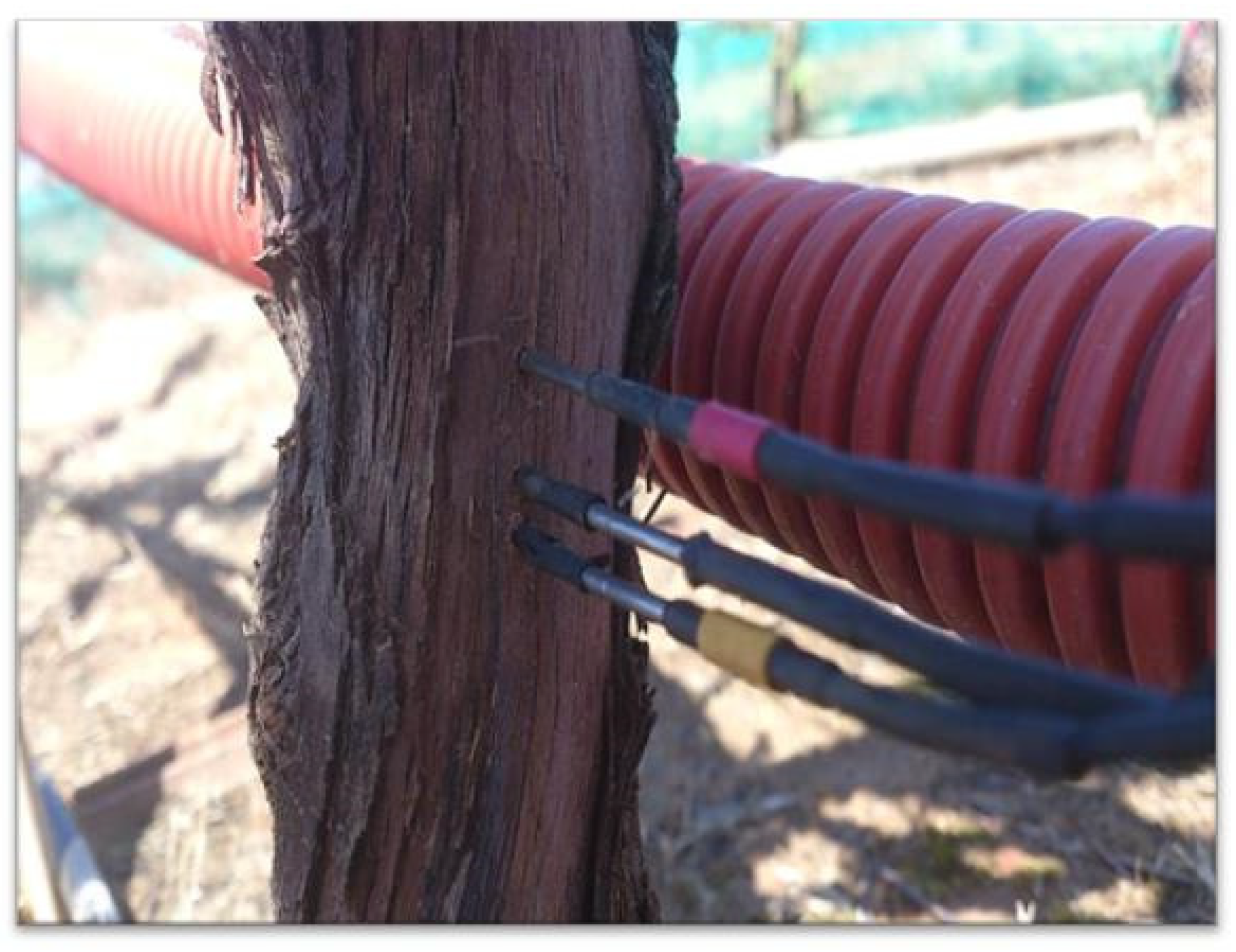
2.5. Water Consumption

We measured the ETc directly in the weighing lysimeter (Figure 1), where we reproduced the growing conditions of two vines in the experimental vineyard. We calculated this ETc from the difference in weight in the lysimeter between two consecutive measurements, adjusted to the equivalent area of an individual vine [6]. In 2013, it was impossible to obtain the complete evolution of ETc due to technical problems with the lysimeter during that season.
The T of the vines was quantified using sap flow sensors developed and assembled by the IAS-CSIC (Córdoba, Spain). The data was processed using the Prosap 3.1.3. program and using the heat pulse compensation (HPC) method plus the average gradient technique [28], as indicated for sap velocities lower than 12 cm h−1. Eight sap flow sensors (one per vine) were installed in an area of the trunk of the vine free of irregularities at a height of 20 cm from the ground, with prior debarking of the chosen area. We monitored four plants in the experimental irrigation plot in block III, two of them on the vines located in the weighing lysimeter. Furthermore, we installed four sensors on vines in the rainfed treatment in block III.
Each sensor consists of three stainless steel tubes of 2 mm diameter, identified by colors; two are thermocouples, and the third is the heater. The thermocouples are located 10 mm above and 5 mm below the heater (Figure 2). The thermocouples, in turn, consist of 4 measuring segments situated at 5, 15, 25, and 35 mm from the end inserted into the cambium. The heater contains a continuous heating wire and is provided with a precision regulator to stabilize the energy released into the xylem, making it independent of possible voltage fluctuations of the batteries. The system is fitted with a CR1000 datalogger (Campbell Scientific Inc., Logan, UT, USA), programmed to run a measurement cycle every 15 min. Heat pulse velocity values due to the wound effect [32] were corrected considering 2.6 mm wound diameter according to [66], subsequently converted to sap velocity and integrated first along the trunk radius (using the radial velocity curve given by the probe) and then around the azimuth angle [67].
Each month, we determined the diameter of each of the vines at the height of the probe insertion using digital calipers, implementing these values in cm in one of the processing files named DIAM, with the values obtained increased by multiplying them by a factor α = 3, based on an adjustment made during a covering cycle in the weighing lysimeter in 2014. The obtained adjustment of the transpiration responded to the linear equation:
(y =2.6273x − 4.2398; R2 = 0.95; n = 6)
The values obtained were processed using the Prosap 3.1.3 program and averaged to then obtain, from sap flow values in (l h−1), values of daily transpiration (TSF) in mm day−1, or in l vine−1 day−1.

2.6. Soil Evaporation

Soil evaporation was obtained directly from the lysimeter by several covering cycles from May to October during the 2010 season on rain-free days. This covering was done with black plastic to avoid water evaporation from the soil surface, obtain T for those days, and calculate the T/ETo ratio. E was determined using Ke:
Ke = (ETc/ETo) − (T/ETo) = E/ETo
We obtained ETc as the average value of the two days before and after the day the lysimeter was covered, as described in [68], and subsequently established a correlation between the Ke and the ETc of the lysimeter responding to the linear equation:
(Ke = 0.0606 ETc − 0.0689; R2 = 0.65; n = 7)
Thus, crop evapotranspiration was determined by sap flow (ETcSF) as the sum of the TSF and E components.

2.7. Statistical Analysis

The yield results were subjected to a one-factor analysis of variance (ANOVA) for each year, using SPSS version 20 (IBM, Armonk, NY, USA). We performed the correlations using linear regression analysis.
The procedure followed in this study was divided into several stages (Data Collection, Adjustment and Validation), as shown in Scheme 2.

3. Results

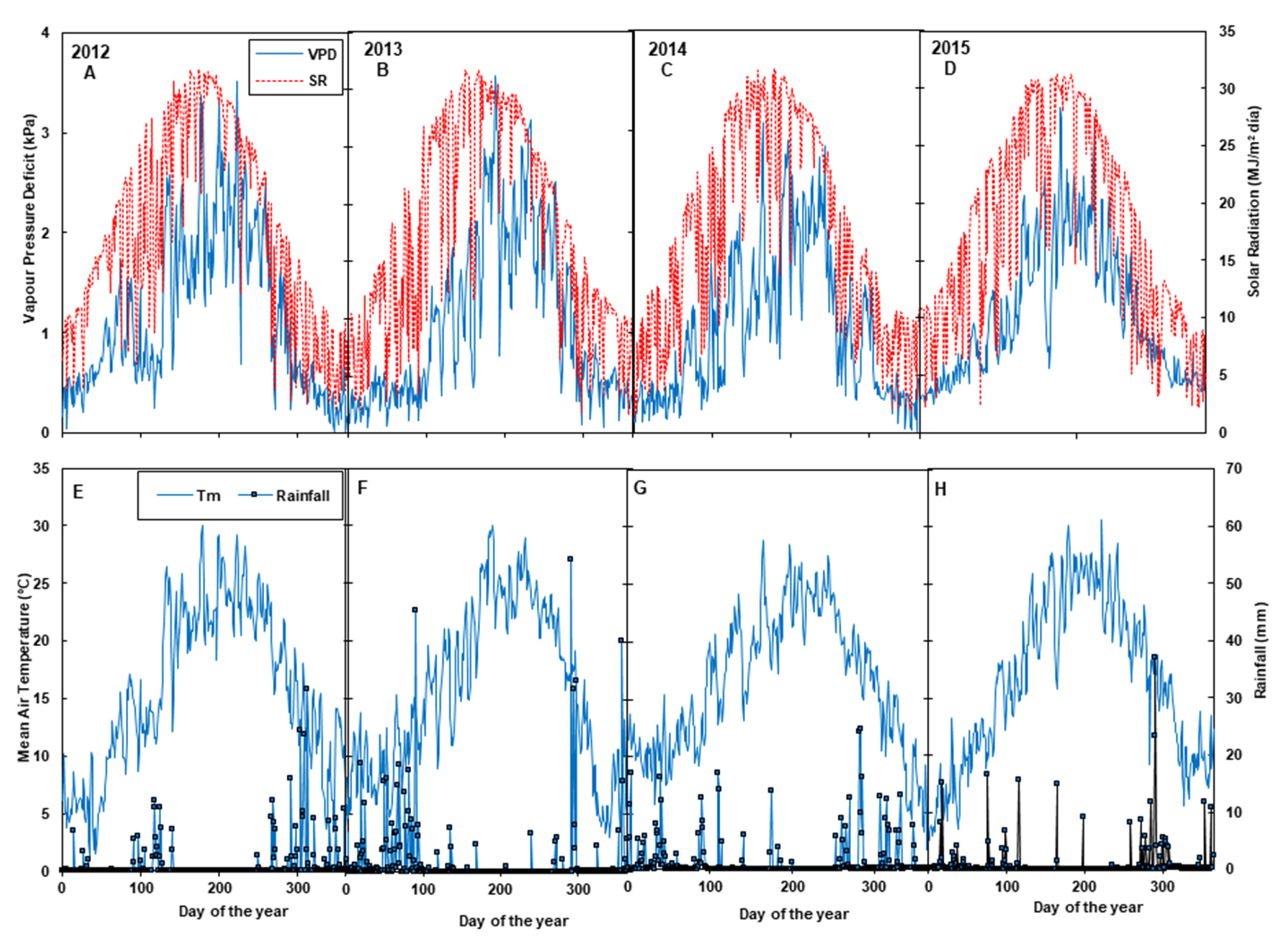
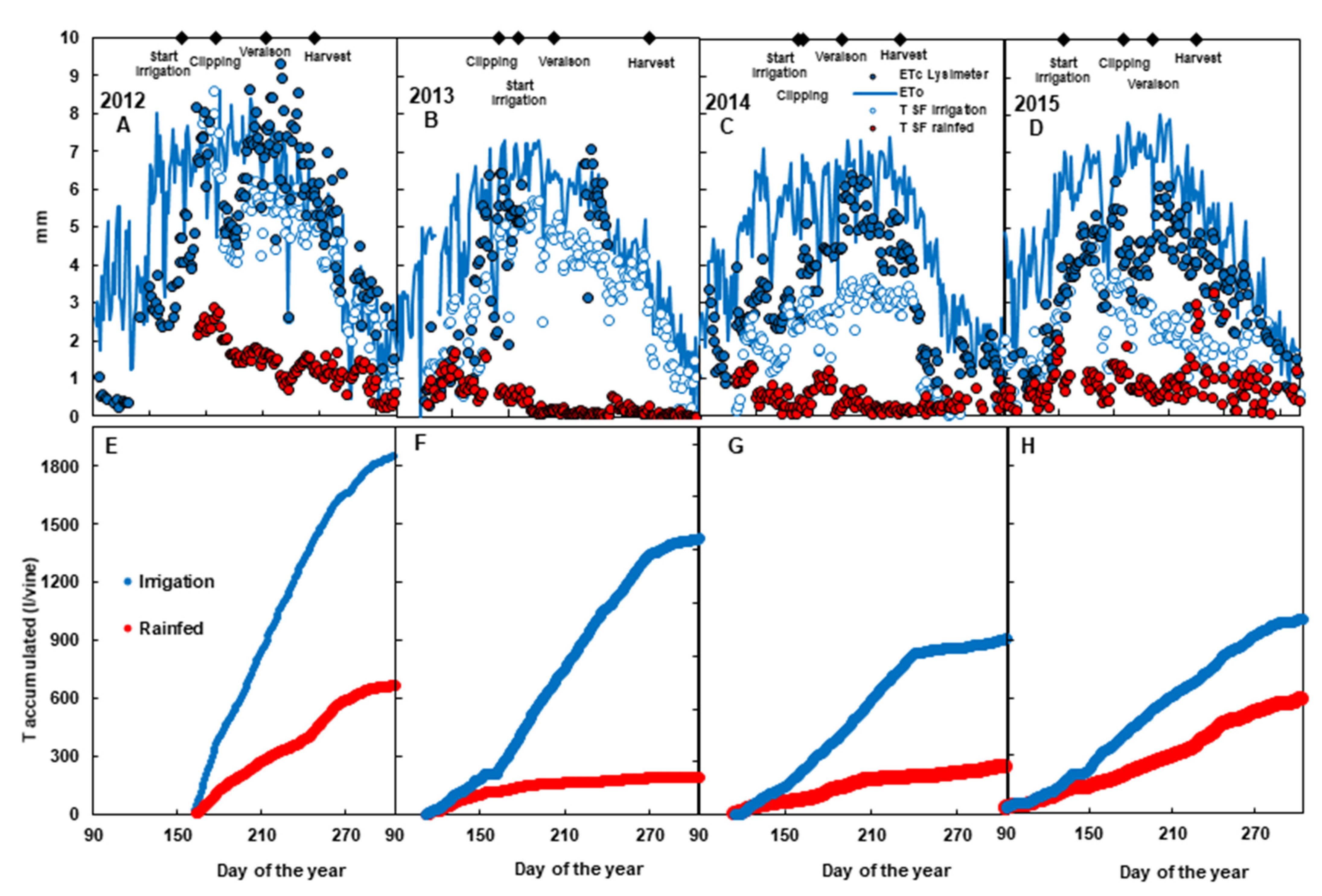
3.1. Weather Conditions

The average annual rainfall was 441 mm, with 2013 being the wettest year with 585 mm and 2015 the driest with 312 mm. Despite these yearly values, the least rainy year during the vegetative period (April–September) was 2013, with 64 mm. However, rainfall was abundant in March, before budbreak (181 mm), and in October (135 mm), close to leaf fall. The years 2012 and 2014 were the wettest years between budbreak and leaf fall, with the same rainfall of 136 mm (Figure 3).
As shown in Figure 3, the seasonal pattern of solar radiation (SR) was similar in the four years. The month with the highest SR was July, with average values ranging from 29.5 MJ m−2 day−1 in 2012 to 27.7 MJ m−2 day−1 in 2014. However, the VPD had the maximum values shifted towards August, except in 2015 when they were reached in July. These maximum values ranged between 3.5 and 3.1 kPa day−1. For the vegetative period of the vines, the minimum values were in April, ranging between 0.7 and 1.0 kPa day−1 (Figure 3). Mean daily temperature (Tm) had a similar pattern to SR, with the highest values ranging from 30.5 °C in 2015 to 28.9 °C in 2014 (Figure 3).

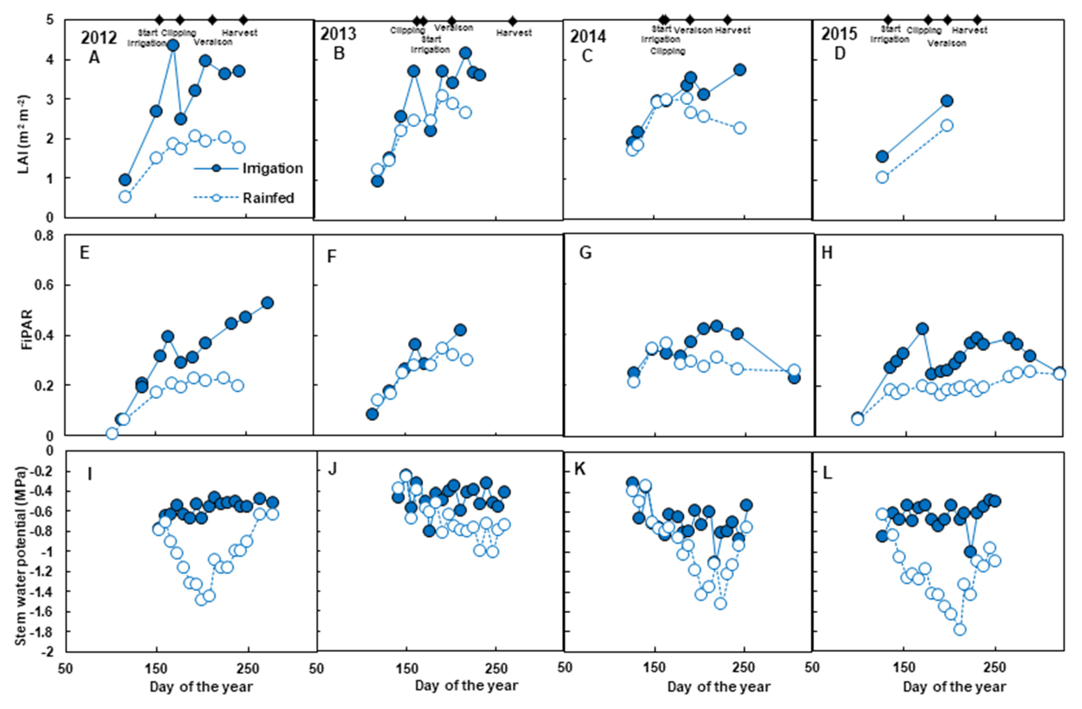
3.2. Vegetative Growth, Water Status, and Yield

The seasonal evolution of LAI, FiPAR and Ψsmd for the two treatments and the four years of study is shown in Figure 4.
The LAI of the irrigation treatment increased after budbreak until clipping, which caused a sharp decrease to recover the increasing trend until veraison, after which it decreased in 2012 and 2014 (Figure 4A–C). The highest LAI value was observed in 2012 in the irrigation treatment before veraison. Around harvest, the LAI of this treatment reached values close to 3.70. In the rainfed treatment, the maximum was 3.12 in 2013, with values at harvest between 1.76 and 2.26 (Figure 4A–C).
Like the LAI, FiPAR increased from budbreak until a sharp decline after clipping, with a subsequent recovery until the last measurements made in 2012 and 2013. In 2014 and 2015, there was a slight recovery of FiPAR post-clipping followed by a stabilization and final drop with leaf senescence. The maximum FiPAR value was reached in the irrigation treatment in 2012 with 0.53 at the end of the season (Figure 4E). In the rainfed treatment, the FiPAR increase was slower than in the irrigation treatment from early stages in 2012 and 2015, reaching stable values before the clipping which were maintained until leaf senescence at the end of the cycle (Figure 4E,H). In 2013 and 2014, the differences between treatments were established later, at day of year (DOY) 192 and 178 in 2013 and 2014, respectively, being lower than in previous years from this point onwards. Before the clipping, the maximum FiPAR rainfed treatment values ranged between 0.20 and 0.37 in the years under study, with this treatment reaching values of around 0.25 at the end of the measurement period (Figure 4E–H).
The most noteworthy differences between treatments in terms of vegetative development correspond to 2012, both in LAI and FiPAR, while the least differences were observed in 2013.
Regarding water status, the irrigation treatment vines maintained constant Ψsmd values throughout the cycle, around −0.6 MPa, except in 2014 when we observed a slight initial decrease, stabilizing after 150 DOY at around −0.7 MPa (Figure 4I–L). Although the rainfed treatment achieved significantly lower Ψsmd values in all years than the irrigation treatment, there were notable differences between years, with minimum values ranging from −1.0 MPa in 2013 to −1.8 MPa in 2015. We observed the most significant differences between treatments in the 2012 and 2015 seasons, which began to separate at around DOY 150. The minimum values of the rainfed treatment were reached around veraison when we observed the greatest differences with the irrigation treatment. A subsequent recovery brought the Ψsmd of both treatments closer but without reaching the same level (Figure 4I,L). In 2013 and 2014, there were no differences between treatments up to DOY 191 and DOY 178, respectively. In 2013, there were constant differences between the irrigated and rainfed treatments from veraison onwards. In 2014, the Ψsmd recovery of the rainfed treatment at the end of the cycle again equaled the potentials of both treatments (Figure 4J,K).
Yields in the irrigation treatment ranged between 10,864 and 28,689 kg ha−1 in 2014 and 2013, respectively, and in the rainfed treatment between 8243 kg ha−1 in 2015 and 17,300 kg ha−1 in 2013 (Table 1). The year 2013 was the most productive in both treatments. In 2014, both treatments had similar yield and this was the only year in which no significant effect of irrigation management was found (Table 1).

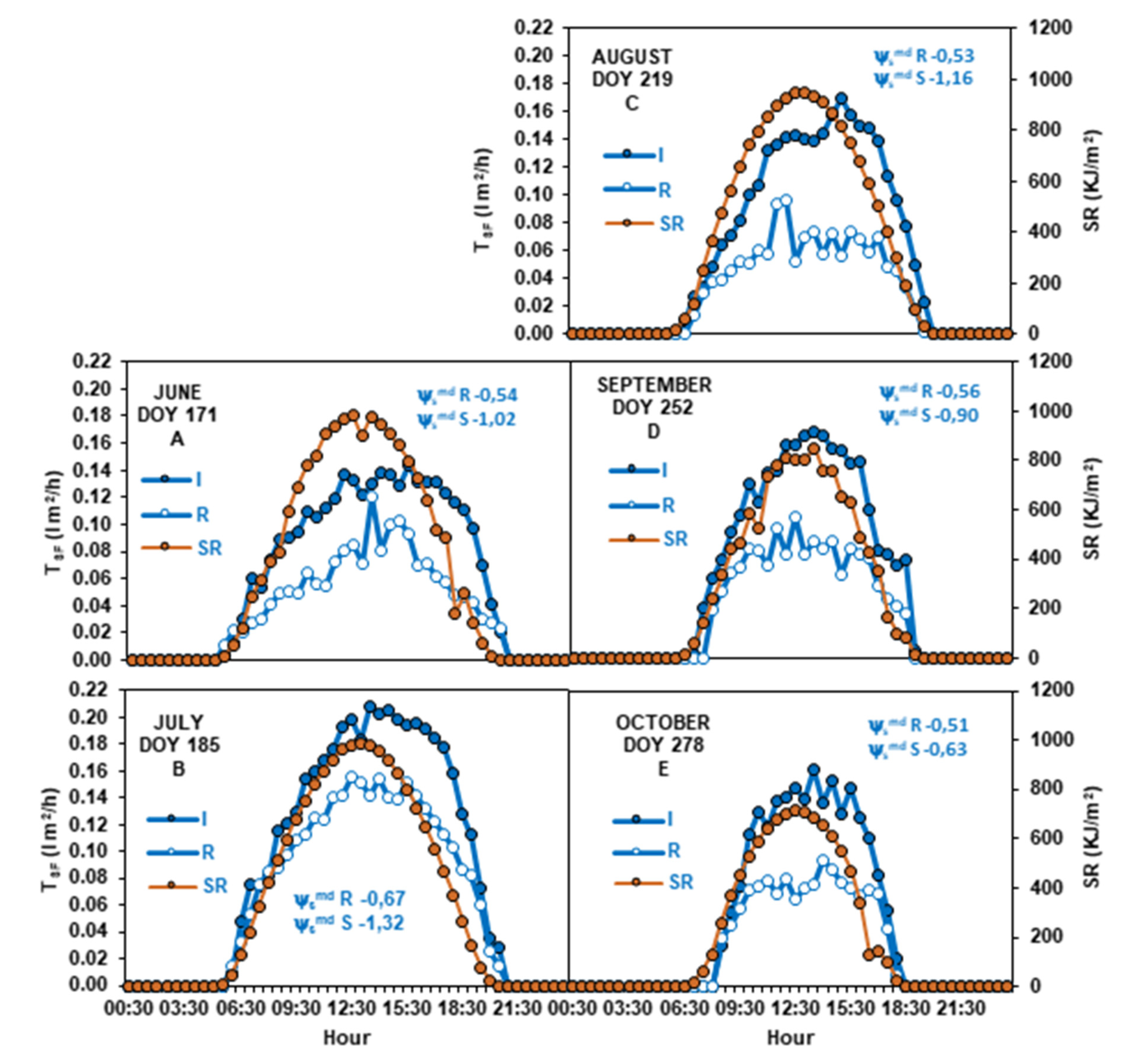
3.3. Evaporation, Transpiration, and Evapotranspiration

The seasonal ETo was different in every year, with the highest values obtained in 2012, mainly up to veraison (Figure 5A–D). In all years there was a similar seasonal trend between ETo, ETcLys, and TSF, but in the last two years the separation between ETo and ETcLys and TSF was greater than in the other years. The seasonal evolution of TSF in the lysimeter plants, under non-water-limiting conditions, had the same tendency as ETcLys, but with lower values (Figure 5A–D). Both processes had close values prior to the first irrigation, mainly in 2015 until DOY 133 (Figure 5D). Both parameters decreased with the clippings and increased until veraison, with a subsequent plateau phase. The decreasing trend started before ripening and continued to leaf fall (Figure 5A–D). TSF was noticeably lower in rainfed plants than irrigated ones, with values between 0 and 1 mm/day during most of the season in 2013 and 2014, and higher values in 2012 and 2015. Differences between treatments started early in the season around the beginning of flowering (DOY 130), and even before the first irrigation in 2013 and 2014 (Figure 5A–D) and without having yet produced a differentiation in Ψsmd values due to irrigation in these years (Figure 4I–L).
The cumulative TSF (Figure 5E–H) for the irrigation treatment increased after budbreak in all years and remained with the same slope until harvest. From this point on, in 2012 and 2015 the trend was maintained, while in 2013 and 2014 a change in the slope can be observed with a drop in TSF. In the rainfed treatment, the slope was lower and with no drastic changes in the trend along the season. Once again, the years 2012 and 2015 differed from 2013 and 2014, with lower cumulative transpiration in the two central trial years (Figure 5E–H).
Table 2 shows the average daily values of different parameters for the months from April to October each year. In the first two years, part of the data were lost (Table 2). In the first two years, ETcSF was higher than ETcLys, while in the last two years ETcLys had slightly higher values in May to October in 2014 and July to September in 2015 (Table 2). Considering the average of the four years, the ETc obtained by both procedures was very similar (Table 3). Consequently, the crop coefficient (Kc) values obtained in both cases were similar when considering the four years as a whole. The maximum values of 0.85 and 0.82 for ETcLys and ETcSF, respectively, were in August (Table 3).
E was higher in 2012 than in subsequent years, reaching 2.29 mm day−1 as the mean value for August (30% and 33% of ETcLys and ETcSF, respectively) (Table 2). The TSF in the irrigation treatment was variable, with the highest daily values reached in all years in July but with notable differences between the first two years close to 5 mm day−1, while in the latter years the maximum barely exceeded 3 mm day−1 (Table 2). The TSF in the rainfed treatment was much lower than in the irrigated treatment in all cases, but without a clearly defined seasonal pattern.
Figure 6 shows the daily evolution of TSF per unit of leaf area for different days in the months under study in 2012. As can be seen, there is a certain parallelism between the daily evolution of TSF and SR in the early morning hours, with a certain shift of the maximum values of TSF towards the afternoon. The number of hours of sunshine affects TSF, so that in June the daily transpiration period was 14 h and 30 min (Figure 6A), while in October it was reduced to 10 h (Figure 6E). From the first measurements in June 2012 (Figure 6A), the rainfed treatment had a lower TSF per unit leaf area than the irrigation treatment. However, the daily evolution followed the same trend in both treatments in all months, with no abrupt restriction of TSF detected in the rainfed treatment, even with Ψsmd of −1.3 MPa (Figure 6B), as was observed in 2013 and 2014 (Figure 5B,C).

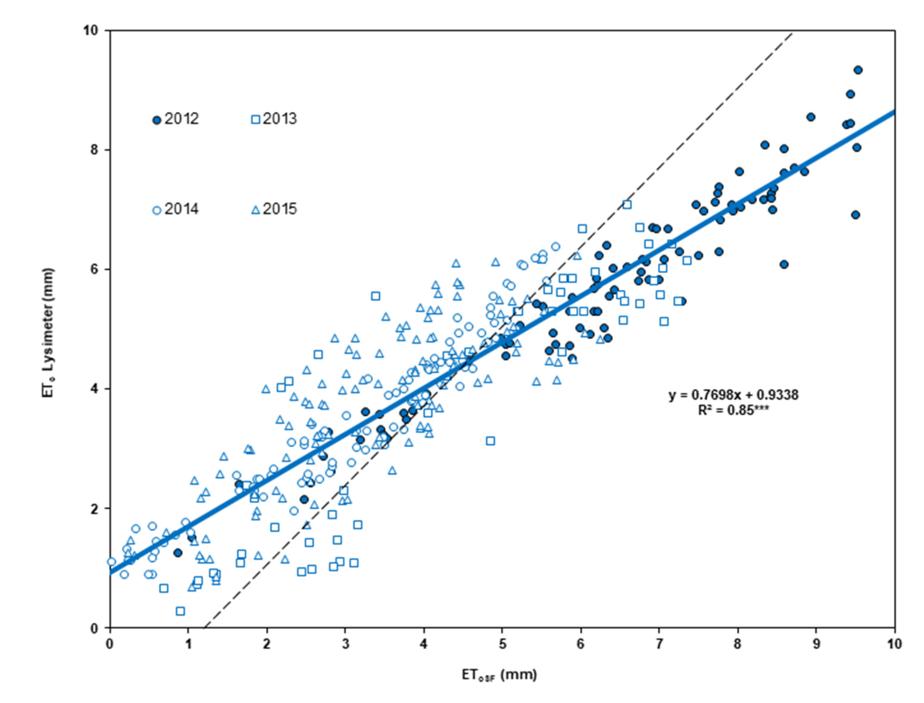
3.4. Relationship between Methodologies for Determining ETc

The relationship between ETcSF obtained from the sum of its components TSF and E and ETcLys obtained directly from a weighing lysimeter for the four years of the trial is presented in Figure 7. The linear regression was highly significant with R2 = 0.85 but did not coincide with the 1:1 line. With low values, ETcLys was higher than ETcSF, while the situation was reversed for high values. As seen previously in Table 2, in the first two years ETcSF overestimated ETc relative to the lysimeter measurements.
The year 2012 was the year in which the greatest amplitude of values was obtained, with maximum values higher than 9.0 mm, while in the other years the maximum values were between 6.0 and 7.0 mm.
With all this, the validation of the adjustments made was satisfactory, as it was possible to reproduce ETcLys by means of the sap flow sensor methodology and evaporation modeling.

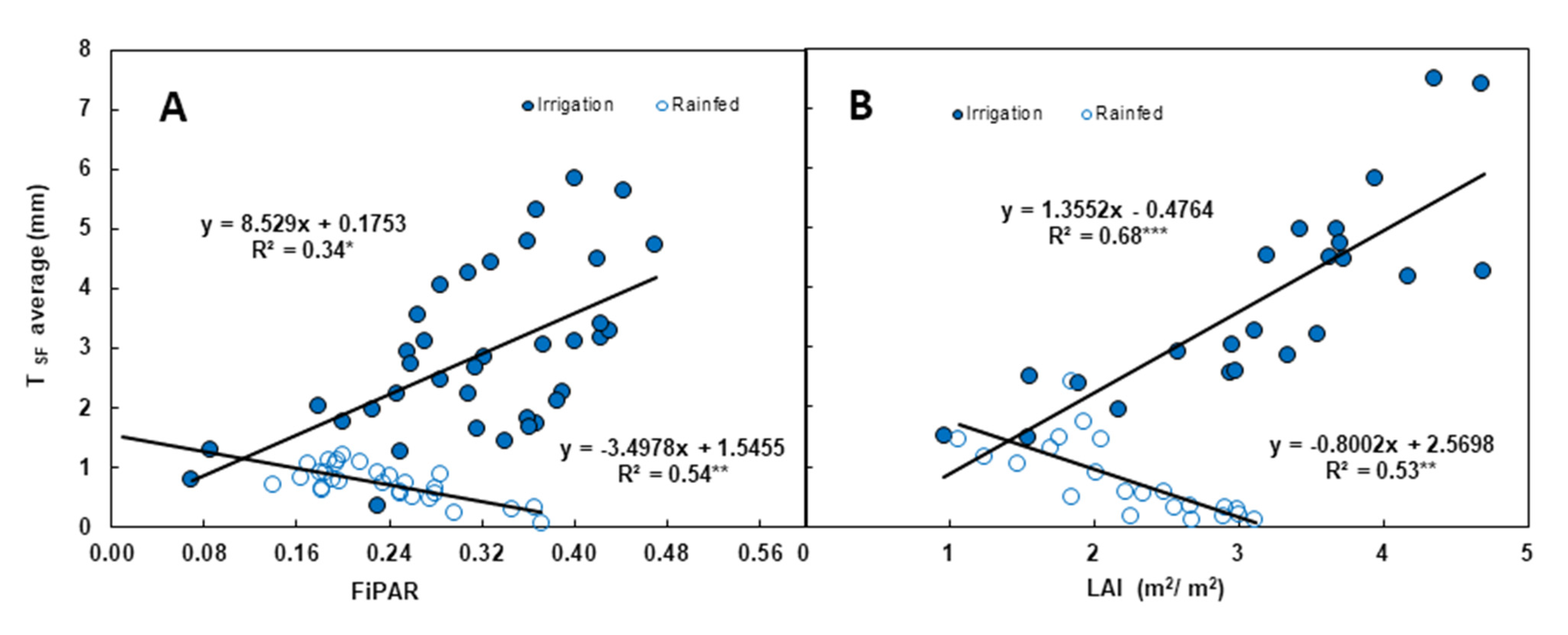
3.5. Relationship between Vegetative Growth and TSF

The relationship between TSF and the measured vegetative growth indexes, FiPAR and LAI, for the two treatments in the four years of the trial is presented in Figure 8. The increase in FiPAR and LAI in the irrigation treatment was accompanied by a rise in TSF. This relationship was more robust with LAI with an R2 = 0.68 (Figure 8B) than for FiPAR R2 = 0.34 (Figure 8A). In the rainfed treatment, the TSF decreased as the vegetation on the vines increased. The correlation coefficients obtained for FiPAR and LAI were similar: R2 = 0.54 and 0.53 for FiPAR and LAI, respectively (Figure 8A,B).

4. Discussion

Although calculations of vineyard water requirements consider both evaporation from the soil surface and transpiration from the vines and living plant covers, only the water transpired by the vines influences vine productivity so that efficient irrigation is achieved when most of the water applied is consumed as transpiration [69]. Therefore, the quantification of transpiration provides the necessary information to improve water use both in high and low water availability conditions. Although sap flow sensors determine plant water consumption, it is necessary to adjust this methodology to obtain accurate values, especially when the aim is to evaluate plant response to different factors. The regulation of vine water relations is an essential tool for managing vineyard quality, which depends on the availability of water and the plant mechanisms involved in regulating gas exchange in the plant canopy.
In this work, we evaluated the use of sap flow measurements in vineyards, both for the accurate assessment of water consumption, with the support of a weighing lysimeter as a reference, and to analyze the effect of water stress on the vines on the daily and seasonal patterns of transpiration.

4.1. Adjustment and Evaluation of Sap Flow Sensors to Determine Vine’s Transpiration

Although different authors have proposed the use of sap flow measurements to quantify water losses by transpiration in grapevines [19,33,34,35], as in other woody species [27,29,30,31,32,66], direct calibrations give reliability to the measures. In this work, by having a weighing lysimeter it was possible to establish a calibration coefficient of α = 3. Although we obtained this coefficient on the two lysimeter vines, the values and trends of the sap flow rates of the four irrigated vines, together with the rainfed vines, suggest that the fit was acceptable for all of them. Other authors [70] indicated the need to establish a calibration coefficient (α) for each year and sensor, which may have reduced the adjustment obtained in this work by establishing a single coefficient for all years and sensors.

4.2. Quantification of ETc in Vineyards by Sap Flow Measurements

The ETcSF had a good correlation with ETcLys (R2 = 0.85) (Figure 7). The most remarkable feature is the underestimation of this methodology for values lower than 4.5 mm day−1. This may be due to a low estimation of evaporation in periods when rainfall is common, the initial and final stages of cultivation (Figure 3), wetting the entire soil surface and, therefore, increasing the evaporative component within the water consumption of the vineyard [5]. This situation is not included in the proposed evaporation model. As shown in Figure 7, we obtained the best fit between the two ETc determination methodologies in 2012, which was the year in which there were fewer rainfall events during cultivation and when we had no sap flow data until July, which resulted in an R2 value of 0.93 (data not shown). After budbreak in 2013, a year characterized with low crop water consumption and high precipitation during spring, ETcSF was proportionally higher than ETcLys. These observations point to errors in the quantification of E, both due to overestimation and underestimation, and whose relative importance depends on factors such as rainfall and soil wetting and exposure to solar radiation. Therefore, they highlight the need to improve the quantification of E and its contribution to ETc under different circumstances, as already pointed out by [6] under the same conditions.
The highest values of the transpiration coefficient (KT) (calculated as the ratio of TSF to ETo) obtained in this work were significantly lower than the highest basal coefficient (Kcb) obtained by [6] (KT between 0.63 and 0.65, compared to 1 for Kcb), except for 2012 when similar values were reached. Kcb is usually calculated from lysimeter ETc measurements when the top soil layer is dry (ETc ≈ ETcb, zero evaporation), a condition that is hard to reach with drip irrigation due to the high irrigation frequency.
TSF values were similar to those obtained by [71] for cv. Shiraz in the summer months with maximum values around 3.0 mm day−1 versus the 4.0 and 3.6 mm day−1 for July and August, respectively, obtained in our study (Table 3). However, our results were appreciably higher than those obtained by [19] for a set of varieties and water status with values ranging between 0.3 and 2.0 mm day−1 versus the 0.1 and 5.2 mm day−1 obtained in our study (Table 2). These higher values could be due to the absence of water stress observed in part of the vines monitored in our study.
The evaluated water consumption parameters followed a seasonal pattern similar to other studies [6,72]. The difference in values from other studies might be due to the increased vegetative growth and consequently the increased water consumption during July and August (Kc = 0.78–0.85) (Table 3). In the summer months (DOY 152–243), the greatest differences between ETc and TSF were observed (Figure 5A–D), coinciding with the application of irrigation, which increased evaporation due to the increase in the wetted soil surface. This gap between ETc and TSF was because these months were those with the highest evaporative component (Table 2 and Table 3), with this evaporation reaching a maximum in July and August (DOY 182–243). The maximum values of solar radiation and air temperature, determining factors for evaporation, were recorded in these months (Figure 3). These results are similar to those obtained for a vineyard of the same variety by [5], although in our case we obtained lower evaporation rates in the early stages of crop development period.
The maximum values of E in the irrigation months (Table 2 and Table 3) show the inefficiency of high irrigation frequencies in semi-arid climates as they lead to significant evaporation losses [5], with maximum values of 30% and 33% of the total value of ETc in June, July, and August, in accordance with the findings of [5] for high irrigation volumes.
Moreover, we observed the effect of pruning on transpiration, both in the weighing lysimeter and in the data obtained using sap flow probes (Figure 5A–D). There was a decrease proportional to the leaf area removed by green pruning, which agrees with previous observations in vines [6] and other woody crops [2,57,67,73].

4.3. Relationship between Transpiration and Vegetative Growth of Grapevines

Crop transpiration is closely related to canopy development under non-water-limiting conditions [2,6,57,67,73], with a maximum stomatal aperture under these conditions with full illumination and high relative humidity [74]. In this study, TSF in the irrigation treatment increased from budbreak with increasing LAI and FiPAR and decreased sharply with the clippings (Figure 4A–H). Comparing relationships between LAI and FiPAR with TSF in the irrigation treatment with those obtained by [6] with Kcb, in both cases there is a better relationship with LAI than with FiPAR. In the rainfed treatment, dispersion is lower since, when stomatal closure occurs, environmental conditions do not have such a strong influence on vine transpiration. Contrary to the irrigation treatment, in the rainfed treatment, the greater development of the canopy reduces TSF (Figure 8A,B), as stomatal closure is necessary for the plant to defend itself against water limitation [75]. Under conditions of low water availability, a larger canopy size means higher water demand and faster consumption of reserves, leading to more severe stress. Under these conditions, a series of plant mechanisms that control transpiration through stomatal closure comes to the fore [76].

4.4. Evaluation of Vineyard T Response under Water-Limiting and Non-Water-Limiting Conditions

The conditions in which the strains develop (environmental conditions and water availability) determine the canopy size (number of leaves, size, and arrangement) and characteristics (number and size of stomata) [77], as well as the hydraulic system of the plant [78], and therefore, the transpiration potential at a given time. In grapevines, stomatal conductance depends on environmental conditions during the early stages of leaf development, as it sets the upper limit of conductance by modulating the density and size of the stomata, the current conditions, and the source-to-sink ratio [77]. When vines develop under high-temperature conditions in the absence of water deficit, they can increase canopy growth with increased transpiration [79]. In the year 2012, with higher temperature and radiation after budbreak, the irrigation treatment had the highest LAI and FiPAR values relative to subsequent years and possibly explains why the highest TSF values were reached in this year (Figure 5E–H). The scarcity of previous rains in 2012 increased the differences between treatments. However, in 2013, although the temperature was also high in the initial stages, radiation was lower, with a higher number of cloudy days, and rainfall was higher, which reduced the differences in canopy growth between the two treatments. As mentioned above, a larger canopy size under stress conditions resulted in tighter control of transpiration [79]. Differences in TSF were observed among the treatments studied in all years (Figure 5A–D), reaching the highest values in 2012 (Figure 5A).The rainfed treatment presented an anhisohydric behavior in 2012 and 2015, while in 2013 and 2014 its behavior was isohydric, with a drastic decrease in transpiration to reduce water losses in the vines (Figure 5A–D). These results further the controversy of whether the grapevine (Vitis vinifera L.) presents an isohydric or anisohydric behavior [80,81,82]. This different behavior found in our study could be due to environmental conditions [83,84] and the stage of crop development at which adverse conditions occur [85].
The daily change in transpiration agrees with the daily change in SR for irrigation treatment (Figure 6). Stomatic conductance is of particular importance in the control of transpiration in grapevine, which, under non-water-limiting conditions, has a good coupling with the atmosphere [86]. Transpiration intensity in grapevine depends on water vapor pressure differences between the atmosphere and the sub-stomatic chamber. T in irrigated vines is influenced by the VPD [79,87,88]. This fact was confirmed in this study, obtaining the highest transpiration rates in the irrigated vines when the highest VPD were recorded and decreasing as the VPD decreased (Figure 3A–D and Figure 5A–D).
We also noted, coinciding with the study of [89], that transpiration is related to illumination since it is proportional to the radiation received, increasing in the central hours of the day [74]. T increased from early in the morning in the irrigated vines, reaching a maximum value at around 14:00 h, before decreasing from 16:00 h onwards (Figure 6), which agrees with what was observed by [90]. On the other hand, in the rainfed vines there was no significant decrease after 8:00 h, as also indicated by [90], but showed a different behavior depending on the year, with anisohydric behavior in 2012 (Figure 6) and isohydric behavior in 2013 and 2014 when a significant decrease in transpiration was observed in rainfed vines (Figure 5).
Under irrigated conditions, the Ψsmd was maintained at around −0.6 MPa, except in 2014 when there was a slight seasonal decrease (Figure 4I–L). Despite maintaining high values of Ψsmd and similarity between years, the TSF of the irrigation treatment was different from year to year, both due to differences in plant canopy size (Figure 4A–H) and consumption per unit leaf area (Figure 4). In the rainfed treatment, interannual differences in the Ψsmd of the vines must also be added (Figure 4I–L). Circumstances, which have already been highlighted in previous works on this same vineyard [64], highlight the importance of considering weather conditions when planning the agronomic management of the vineyard. In the years 2012 and 2015, in the rainfed vines, there came a time after veraison water stress fell with decreasing evaporative demand (Figure 5A,D), improving the Ψsmd of the vines (Figure 4I,L),which indicates a coupling of the vines with the atmosphere, as found for deciduous trees by some authors [91], with the atmosphere conditioning the water status of the rainfed vines. This fact was less palpable in 2014 and inappreciable in 2013 (Figure 4J–K), manifesting an isohydric behavior.
In other fruit crops, some authors have observed that crop load affects stomatal aperture [57,92,93,94,95], also affecting transpiration in woody crops [66,86]. This effect was not observed in this work since the yield of 2013 was higher than the other three years (which had similar yield values), whereas the highest transpiration values corresponded to 2012. On the other hand, a progressive decrease in transpiration was observed after the harvest, as was found for this same vineyard by [6], a decrease that in some years began even before the harvest. Therefore, there does not seem to be a stomatal closure after the harvest as has been observed in fruit trees such as peach, apple, pear and plum [57,92,93,94,95].
The main insecurity of the methodology proposed for the calculation of ETc in vineyards comes, on the one hand, from the lack of reliability of the evaporation model at certain times of the crop cycle, and on the other hand, from the convenience of establishing annual calibrations for each sensor individually.

5. Conclusions

1ª. The use of a single “α” for all years and sensors gave satisfactory results, but with a deviation that could perhaps have been reduced by individualizing α for each sensor and year.
2ª. The results obtained in the four years of study show that the sap flow sensor methodology, along with the HPC methodology plus the average gradient technique, are useful for quantifying vineyard water consumption, as they provide a good fit with the data obtained directly from a weighing lysimeter.
3ª. Evaporation is an essential component of vineyard water consumption. It is necessary to develop efficient models for its determination and irrigation management to minimize its weight in vineyard water consumption.
4ª. A close positive relationship between vegetative development and water consumption, in the absence of water stress, has been demonstrated. In contrast, under rainfed conditions, this relationship is negative.
5ª. The isohydric or anisohydric behavior of the vineyard is greatly influenced by irrigation management and the environmental conditions of each year. In high initial productive and vegetative expectations, if water inputs do not support these expectations during the season the grapevine (Vitis vinifera L.) shows an isohydric behavior.

Author Contributions

L.A.M. (≈65%), literature review, planning and execution of experimental work, processing of data, discussion of results and writing of the paper; D.U. (≈15%), discussion of results and paper revision; M.d.H.P. (≈20%), project coordinator, planning of experimental work and paper revision. All authors have read and agreed to the published version of the manuscript.

Funding

This research was funded by INIA (RTA2012-00029-C02 project) and Junta de Extremadura (PRI IB10049 project).

Acknowledgments

Junta de Extremadura. FEDER (GR18196, Research Group AGA001, LOI1202017/12, LOI1302020/1 and CCESAGROS projects).

Conflicts of Interest

The authors declare no conflict of interest.

References

  1. Fereres, E.; Evans, R.G. Irrigation of fruit trees and vines: An Introduction. Irrig. Sci. 2006, 24, 55–57. [Google Scholar] [CrossRef]
  2. Ayars, J.E.; Johnson, R.S.; Phone, C.J.; Trout, T.J.; Clark, D.A.; Mead, R.M. Water use by drip-irrigated late-season peaches. Irrig. Sci. 2003, 22, 187–194. [Google Scholar] [CrossRef]
  3. Allen, R.G.; Pereira, L.S.; Raes, D.; Smith, M. Crop Evapotranspiration: Guidelines for Computing Crop Water Requirements. Irrigation and Drainage, 56; FAO: Rome, Italy, 1998. [Google Scholar]
  4. Doorenbos, J.; Pruitt, W.O. Crop water requirements. FAO Irrigation and Drainage Paper nº 24; FAO: Rome, Italy, 1975. [Google Scholar]
  5. Montoro, A.; Mañas, F.; López-Urrea, R. Transpiration and evaporation of grapevine, two components related to irrigation strategy. Agric. Water Manag. 2016, 177, 193–200. [Google Scholar] [CrossRef]
  6. Picón-Toro, J.; González-Dugo, V.; Uriarte, D.; Mancha, L.A.; Testi, L. Effects of canopy size and water stress over the crop coefficient of a “Tempranillo” vineyard in south-western Spain. Irrig. Sci. 2012, 30, 419–432. [Google Scholar] [CrossRef] [Green Version]
  7. Williams, L.E.; Ayars, J.E. Grapevine water use and the crop coefficient are linear functions of the shaded area measured beneath the canopy. Agric. For. Meteorol. 2005, 132, 201–211. [Google Scholar] [CrossRef]
  8. Jackson, D.I.; Lombard, P.B. Environmental and management practices affecting grape composition and wine quality- A review. Am. J. Enol. Vitic. 1993, 44, 409–430. [Google Scholar]
  9. Vadour, E. Les terroirs viticoles. Definitions, Characterisation, Protection; Dunod: Paris, France, 2003; 293p. [Google Scholar]
  10. Praeger, J.H.; Hatfield, J.L.; Aase, J.K.; Pikul, J.L. Bowen-ratio comparisons with lysimeter evapotranspiration. Agron. J. 1997, 89, 730–736. [Google Scholar] [CrossRef] [Green Version]
  11. Hatfield, J.L. Methods of estimating evapotranspiration. In Irrigation of Agricultural Crops. Agron Monogr Nº. 30; Stewart, B.A., Nielson, D.R., Eds.; ASA-CSSA-SSSA: Madison, WI, USA, 1990; pp. 435–474. [Google Scholar]
  12. Andreu, L.; Hopmans, J.W.; Schwankl, L.J. Spatial and temporal distribution of soil water balance for a drip-irrigated almond tree. Agric. Water Manag. 1997, 35, 123–146. [Google Scholar] [CrossRef]
  13. Abrisqueta, J.M.; Ruiz, A.; Franco, J.A. Water balance of apricot trees (Prunus armeniaca L. cv. Búlida) under drip irrigation. Agric. Water Manag. 2001, 50, 211–227. [Google Scholar] [CrossRef]
  14. García-Petillo, J.R.; Castel, J.R. Water balance and crop coefficient estimation of a citrus orchard in Uruguay. Span. J. Agric. Res. 2007, 5, 232–243. [Google Scholar] [CrossRef] [Green Version]
  15. Moreno, F.; Vachaud, G.; Matín-Aranda, J.; Vauclin, M.; Fernádez, J.E. Balance hídrico en un olivar con riego gota a gota. Resultados de cuatro años de experiencias. Agronomie 1988, 8, 521–537. [Google Scholar] [CrossRef] [Green Version]
  16. Samperio, A.; Moñino, M.J.; Marsal, J.; Prieto, M.H.; Stöckle, C.O. Use of CropSyst as a tool to predict water use and crop coefficient in Japanese plum trees. Agric. Water Manag. 2014, 146, 57–68. [Google Scholar] [CrossRef]
  17. De Teixeira, A.H.C.; Bastiaansen, W.G.M.; Basso, L.H. Crop water parameters of irrigated wine and table grapes to support water productivity analysis in the Sao Francisco river basin, Brazil. Agric. Water Manag. 2007, 94, 31–42. [Google Scholar] [CrossRef]
  18. Zhang, B.; Kang, S.; Li, F.; Tong, L.; Du, T. Variation in vineyard evapotranspiration in arid region of northwest China. Agric. Water Manag. 2010, 97, 1898–1904. [Google Scholar] [CrossRef]
  19. Ferreira, M.I.; Silvestre, J.; Conceicao, N.; Malhiero, A.C. Crop and stress coefficients in rainfed and deficit irrigation vineyards using sap flow techniques. Irrig. Sci. 2012, 30, 433–447. [Google Scholar] [CrossRef]
  20. Poblete-Echeverria, C.; Ortega-Farias, S. Estimation of actual evapotranspiration for a drip-irrigated Merlot vineyard using a three-source model. Irrig. Sci. 2009, 28, 65–78. [Google Scholar] [CrossRef]
  21. Ortega-Farias, S.; Carrasco, M.; Olioso, A.; Acevedo, C.; Poblete, C. Latent heat flux over Cabernet Sauvignon vineyard using the Shuttleworth and Wallace model. Irrig. Sci. 2007, 25, 161–170. [Google Scholar] [CrossRef]
  22. Parry, C.K.; Shapland, M.; Williams, L.E.; Calderon-Orellana, A.; Snyder, R.L.; Paw, U.K.T.; McElrone, A.J. Comparison of a stand-alone surface renewal method to weighing lysimeter and eddy covariance for determining vineyard evapotranspiration and vine water stress. Irrig. Sci. 2019, 37, 737–749. [Google Scholar] [CrossRef]
  23. Granier, A. Une nouvelle méthode pour la mesure du flux de sève brute dansle tronc des arbres (A new method of sap flow measurement in tree stems). Ann. For. Sci. 1985, 42, 193–200. [Google Scholar] [CrossRef]
  24. Wullschleger, S.D.; Meinzer, F.C.; Vertessy, R.A. A review of whole-plant water use studies in trees. Tree Physiol. 1998, 18, 499–512. [Google Scholar] [CrossRef] [Green Version]
  25. Sakurai, T.; Abe, J. A heat balance for measuring water flow rate in stems of intact plants and its application to sugarcane plants. Jpn. Agric. Res. Q. 1985, 19, 92–97. [Google Scholar]
  26. Smith, D.M.; Allen, S.J. Measurement of sap flow in plant stems. J. Exp. Bot. 1996, 47, 1833–1844. [Google Scholar] [CrossRef] [Green Version]
  27. López-Bernal, A. Efectos del Déficit Hídrico Sobre el Flujo de Savia y la Conductancia Estomática en Frutales. Ph.D. Thesis, Departamento de Agronomía. Universidad de Córdoba, Córdoba, Spain, 2015. [Google Scholar]
  28. Testi, L.; Villalobos, F.J. New approach for measuring low sap velocities in trees. Agric. For. Meteorol. 2009, 149, 730–734. [Google Scholar] [CrossRef]
  29. Fernández, J.E.; Durán, P.J.; Palomo, M.J.; Díaz-Espejo, A.; Chamorro, V.; Girón, I.F. Calibration of sap flow estimated by the compensation heat pulse method in olive, plum and orange trees: Relationships with xylem anatomy. Tree Physiol. 2006, 26, 719–728. [Google Scholar] [CrossRef] [Green Version]
  30. Green, S.R.; Clothier, B.E. Water use of kiwifruit, vines and apple trees by the heat-pulse technique. J. Exp. Bot. 1988, 39, 115–123. [Google Scholar] [CrossRef]
  31. Ortuño, M.F.; García-Orellana, Y.; Conejero, W.; Ruiz-Sánchez, M.C.; Alarcón, J.J.; Torrecillas, A. Stem and leaf water potentials, gas exchange, sap flow, and trunk diameter fluctuations for detecting water stress in lemon trees. Trees 2006, 20, 1–8. [Google Scholar] [CrossRef]
  32. Swanson, R.H.; Whitfield, D.W.A. A numerical analysis of heat pulse velocity theory and practice. J. Exp. Bot. 1981, 32, 221–239. [Google Scholar] [CrossRef]
  33. Fernández, J.E.; Green, S.R.; Caspari, H.W.; Díaz-Espejo, A.; Cuevas, M.V. The use of sap flow measurements for scheduling irrigation in olive, apple and Asian pear trees and in grapevines. Plant Soil 2008, 305, 91–104. [Google Scholar] [CrossRef]
  34. Ginestar, C.; Eastham, J.; Gray, S.; Iland, P. Use of sap flow sensors to schedule vineyard irrigation. I. Effects of post-veraison water deficits on water relations, vine growth, and yield of Shiraz grapevines. Am. J. Enol. Vitic. 1998, 49, 413–420. [Google Scholar]
  35. Intrigliolo, D.S.; Lakso, A.; Piccioni, R. Grapevine cv. ‘Riesling’ water use in the northeastern United States. Irrig. Sci. 2009, 27, 253–262. [Google Scholar] [CrossRef]
  36. Williams, L.E.; Phone, C.J.; Grimes, D.W.; Trout, T.J. Water use of mature Thompson Seedless grapevines in California. Irrig. Sci. 2003, 22, 11–18. [Google Scholar] [CrossRef]
  37. Correlli-Grappadelli, L.; Magnanini, E. A whole-tree system for gas-exchange studies. Hortic. Sci. 1993, 28, 41–45. [Google Scholar] [CrossRef] [Green Version]
  38. Lakso, A.N.; Mattie, G.B.; Nyrop, J.P.; Denning, S.S. Influence of European Red Mite on Leaf and Whole-canopy Carbon Dioxide Exchange, Yield, Fruit Size, Quality, and Return Cropping in “Starkrimson Delicious” Apple Trees. J. Amer. Soc. Hort. Sci. 1996, 121, 954–996. [Google Scholar] [CrossRef] [Green Version]
  39. Poni, S.; Magnanini, E.; Rebucci, B. An automated chamber system for measurements of whole-vine gas exchange. HortScience 1997, 32, 64–67. [Google Scholar] [CrossRef]
  40. Poblete-Echeverria, C.; Ortega-Farias, S.; Zuñiga, M.; Fuentes, S. Evaluation of compensated heat-pulse velocity method to determine vine transpiration using combined measurements of eddy covariance system and microlysimeters. Agric. Water Manag. 2012, 109, 11–19. [Google Scholar] [CrossRef]
  41. Green, S.R. Measurement and modelling the transpiration of fruit trees and grapevines for irrigation scheduling. In Proceedings of the Fifth International Symposium on Irrigation of Horticultural Crops, Mildura, VIC, Australia, 28 August–2 September 2006; Goodwin, I.O.M.G., Ed.; ISHS, Acta Horticulturae No 792: Leuven, Belgium, 2008; pp. 321–332. [Google Scholar] [CrossRef]
  42. Ballester, C.; Castel, J.; Jimenez-Bello, M.A.; Castel, J.R.; Intrigliolo, D.S. Thermo-graphic measurement of canopy temperature is a useful tool for predicting water deficit effects on fruit weight in citrus trees. Agric. Water Manag. 2013, 122, 1–6. [Google Scholar] [CrossRef]
  43. Espadafor, M.; Orgaz, F.; Testi, L.; Lorite, I.J.; Villalobos, F.J. Transpiration of young almond trees in relation to intercepted radiation. Irrig. Sci. 2015, 33, 265–275. [Google Scholar] [CrossRef] [Green Version]
  44. Bonachela, S.; Orgaz, F.; Villalobos, F.J.; Fereres, E. Measurement and simulation of evaporation from soil in olive orchards. Irrig. Sci. 1999, 18, 205–211. [Google Scholar] [CrossRef]
  45. Palomo, M.J.; Díaz-Espejo, A.; Fernández, J.E.; Girón, I.F.; Moreno, F. Using sap flow measurements to quantify water consumption in the olive tree. In Water and the Environment: Innovative Issues in Irrigation and Drainage; Pereira, L.S., Gowing, J.W., Eds.; E&FN Spon: Pereira, Colombia, 1998; pp. 205–212. [Google Scholar]
  46. Bonachela, S.; Orgaz, F.; Villalobos, F.J.; Fereres, E. Soil evaporation from drip-irrigated olive orchards. Irrig. Sci. 2001, 20, 65–71. [Google Scholar] [CrossRef]
  47. Intrigliolo, D.S.; Castel, J.R. Vine and soil-based measures of water status in a Tempranillo vineyard. Vitis 2006, 45, 157–163. [Google Scholar] [CrossRef]
  48. Medrano, H.; Escalona, J.M.J.; Gulías, J.; Flexas, J. Regulation of Photosynthesis of C3 Plants in Response to Progressive Drought: Stomatal Conductance as a Reference Parameter. Ann. Bot. 2002, 89, 895–905. [Google Scholar] [CrossRef] [PubMed]
  49. Girona, J.; Mata, M.; del Campo, J.; Arbonés, A.; Bartra, E.; Marsal, J. The use of midday leaf water potential for scheduling deficit irrigation in vineyards. Irrig. Sci. 2006, 24, 115–127. [Google Scholar] [CrossRef]
  50. Smart, R.E.; Coombe, B.G. Water relations of grapevines. In Water Deficit and Plant Growth; Kozlowski, T.T., Ed.; Academic Press: New York, NY, USA, 1983; Volume 7, pp. 137–196. [Google Scholar]
  51. Williams, L.E.; Dokoozlian, N.K.; Wample, R. Grape. In Handbook of Environmental Physiology of Fruit Crops; Schaffer, B., Andersen, P.C., Eds.; CRC Press Inc.: Boca Raton, FL, USA, 1994. [Google Scholar]
  52. Naor, A. Midday stem water potential as a plant water stress indicator for irrigation scheduling in fruit trees. Acta Hortic. 2000, 1, 447–454. [Google Scholar] [CrossRef]
  53. Bradford, K.J.; Hsiao, T.C. Physiological responses to moderate water stress. In Physiological Plant Ecology II. Encyclopedia of Plant Physiology (New Series); Lange, O.L., Nobel, P.S., Osmond, C.B., Ziegler, H., Eds.; Springer: Berlin/Heidelberg, Germany, 1982; Volume 12/B. [Google Scholar]
  54. Ojeda, H.; Deloire, A.; Wang, Z.; Carbonneau, A. Determinación y control del estado hídrico de la vid. Efectos morfológicos y fisiológicos de la restricción hídrica en vides. Enología 2008, 6, 1–15. [Google Scholar]
  55. Smart, R.E. Principles of grapevine canopy microclimate manipulation with implications for yield and quality. A review. Am. J. Enol. Vitic. 1985, 36, 230–239. [Google Scholar]
  56. Castel, J.R. Evapotranspiration of a drip-irrigated clementine citrus tree in a weighing lysimeter. Acta Hortic. 1997, 449, 91–98. [Google Scholar] [CrossRef]
  57. Girona, J.; del Campo, J.; Mata, M.; Lopez, G.; Marsal, J. A comparative study of apple and pear tree water consumption measured with two weighing lysimeters. Irrig. Sci. 2011, 29, 55–63. [Google Scholar] [CrossRef]
  58. Consoli, S.; O’Connell, N.; Snyder, R. Measurement of light interception by navel orange orchard canopies: Case study of Lindsay, California. J. Irrig. Drain. Eng. 2006, 132, 9–20. [Google Scholar] [CrossRef]
  59. Braun, P.; Schmid, J. Sap flow measurements in grapevines (Vitis vinifera L.) 1. Stem morphology and use of the heat balance method. Plant Soil 1999, 215, 39–45. [Google Scholar] [CrossRef]
  60. Martí, P.; González-Altozano, P.; López –Urrea, R.; Mancha, L.A.; Shiri, J. Modeling reference evapotranspiration with calculated targets. Assessment and implications. Agric. Water Manag. 2015, 149, 81–90. [Google Scholar] [CrossRef]
  61. Williams, L.E.; Baeza, P. Relationships among ambient temperature and vapor pressure deficit and leaf and stem water potentials of fully irrigated, field-grown grapevines. Am. J. Enol. Vitic. 2007, 58, 173–181. [Google Scholar]
  62. Williams, L.E.; Trout, T.J. Relationships among vine- and soil-based measures of water status in a Thompson Seedless vineyard in response to high-frequency drip irrigation. Am. J. Enol. Vitic. 2005, 56, 357–366. [Google Scholar]
  63. Mancha, L.A.; Uriarte, D.; Valdés, E.; Moreno, D.; Prieto, M.d.H. Effects of Regulated Deficit Irrigation and Early Cluster Thinning on Production and Quality Parameters in a Vineyard cv. Tempranillo under Semi-Arid Conditions in Southwestern Spain. Agronomy 2021, 11, 34. [Google Scholar] [CrossRef]
  64. Uriarte, D.; Intrigliolo, D.S.; Mancha, L.A.; Picón-Toro, J.; Valdés, E.; Prieto, M.H. Interactive effects of irrigation and crop level on Tempranillo vines in semi-arid climate. Am. J. Enol. Vitic. 2015, 66, 101–111. [Google Scholar] [CrossRef]
  65. Shackel, K.A. Water relations of woody perennial plant species. J. Int. Sci. Vigne Vin 2007, 41, 121–129. [Google Scholar] [CrossRef] [Green Version]
  66. Villalobos, F.J.; Testi, L.; Orgaz, F.; García-Tejera, O.; López-Bernal, A.; González-Dugo, M.V.; Ballester-Lurbe, C.; Castel, J.R.; Alarcón-Cabañero, J.J.; Nicolás-Nicolás, E.; et al. Modelling canopy conductance and transpiration of fruit trees in Mediterranean areas: A simplified approach. Agric. For. Meteorol. 2013, 171–172, 93–103. [Google Scholar] [CrossRef]
  67. Green, S.R.; Clothier, B.; Jardine, B. Theory and practical application of heat pulse to measure sap flow. Agron. J. 2003, 95, 1371–1379. [Google Scholar] [CrossRef]
  68. Marsal, J.; Girona, J.; Casadesus, J.; Lopez, G.; Stöckle, C.O. Crop coefficient (Kc) for apple: Comparison between measurements by a weighing lysimeter and prediction by CropSyst. Irrig. Sci. 2013, 31, 455–463. [Google Scholar] [CrossRef]
  69. Fereres, E.; Goldhamer, D.A.; Sadras, V. Yield Response to Water of Fruit Trees and Vines: Guidelines. FAO Irrigation and Drainage Paper nº66; FAO: Rome, Italy, 2012; pp. 246–497. [Google Scholar]
  70. Testi, L. Medidas de ET en cultivos leñosos. Praceedings of the Comunicación oral en el Marco de las Jornadas de la Red de Excelencia RidecoRed AGL2017-90666-REDC, Lérida, Spain, 27–28 November 2019. [Google Scholar]
  71. Trambouze, W.; Voltz, M. Measurements and modelling of transpiration of a Mediterranean vineyard. Agric. For. Meteorol. 2001, 107, 153–166. [Google Scholar] [CrossRef]
  72. Johnson, R.S.; Williams, L.E.; Ayars, J.E.; Trout, T.J. Weighing lysimeters aid study of water relations in tree and vine crops. Calif. Agric. 2005, 59, 133–136. [Google Scholar] [CrossRef] [Green Version]
  73. Pereira, A.R.; Green, S.R.; Villa Nova, N.A. Sap flow, leaf area, net radiation and the Priestley–Taylor formula for irrigated orchards and isolated trees. Agric. Water Manag. 2007, 92, 48–52. [Google Scholar] [CrossRef]
  74. Champagnol, F. Éléments de Physiologie de la Vigne et de Viticulture Générale; Le Progrès Agricole et Viticole: Saint Gely du Fesc, France, 1984. [Google Scholar]
  75. Jones, H.G. Physiological aspects of the control of water status in horticultural crops. HortScience 1990, 25, 19–26. [Google Scholar] [CrossRef] [Green Version]
  76. Lavoie-Lamoureux, A.; Sacco, D.; Risse, P.A.; Lovisolo, C. Factors influencing stomatal conductance in response to water availability in grapevine: A meta-analysis. Physiol. Plant 2017, 159, 468–482. [Google Scholar] [CrossRef] [PubMed]
  77. Sadras, V.O.; Montoro, A.; Moran, M.A.; Aphalo, P.J. Elevated temperature altered the reaction norms of stomatal conductance in field-grown grapevine. Agric. Forest Meteorol. 2012, 165, 35–42. [Google Scholar] [CrossRef]
  78. Munitz, S.; Netzer, Y.; Shtein, I.; Schwartz, A. Water availability dynamics have long-term effects on mature stem structure in Vitis vinifera. Am. J. Botany 2018, 105, 1443–1452. [Google Scholar] [CrossRef] [Green Version]
  79. Bonada, M.; Buesa, I.; Moran, M.I.; Sadras, V.O. Interactive effects of warming and water deficit on Shiraz vine transpiration in the Barossa Valley, Australia. Vine Wine 2018, 52, 189–202. [Google Scholar] [CrossRef]
  80. Blanco-Cipollone, F.; Lourenco, S.; Silvestre, J.; Conceicao, N.; Moñino, M.J.; Vivas, A.; Ferreira, M.I. Plant water status indicators for irrigation scheduling associated with iso- and anisohydric behavior: Vine and plum trees. Horticulturae 2017, 3, 47. [Google Scholar] [CrossRef]
  81. Hugalde, I.P.; Vila, H.F. Comportamiento isohídrico o anisohídrico en vides…:¿ Una controversia sin fin? RIA Rev. Investig. Agropecu. 2014, 40, 75–82. [Google Scholar]
  82. Schultz, H.R. Differences in hydraulic architecture account for near isohydric and anisohydric bahaviour of two field-grown Vitis vinifera L. cultivars during drought. Plant Cell Environ. 2003, 26, 1393–1405. [Google Scholar] [CrossRef]
  83. Domec, J.C.; Noormets, A.; King, J.S.; Sun, G.E.; McNulty, S.G.; Gavazzi, M.J.; Bloggs, J.L.; Treasure, E.A. Decoupling the influence of leaf and root hydraulic conductances on stomatal conductance and its sensitivity to vapour pressure deficit as soil dries in a drained loblolly pine plantation. Plant Cell Environ. 2009, 32, 980–991. [Google Scholar] [CrossRef]
  84. Rogiers, S.Y.; Greer, D.H.; Hutton, R.J.; Clarke, S.J. Transpiration efficiency of the grapevine cv. Semillon is tied to VPD in warm climates. Ann. Appl. Biol. 2011, 158, 106–114. [Google Scholar] [CrossRef]
  85. Intrigliolo, D.S.; Castel, J.R. Usefulness of diurnal trunk shrinkage as a water stress indicator in plum trees. Tree Physiol. 2006, 26, 303–311. [Google Scholar] [CrossRef]
  86. Yunusa, I.A.M.; Walker, R.R.; Lovey, B.R.; Blackmore, D.H. Determination of transpiration in irrigated grapevines: Comparison of the heat-pulse technique with the gravimetric and micrometeorological methods. Irrig. Sci. 2000, 20, 1–8. [Google Scholar] [CrossRef]
  87. González, C.M. Estudio Ecofisiológico y Agronómico de Cuatro Sistemas de Conducción de la vid (Vitis Vinifera L.): Cubiertas Vegetales Simples Versus Divididas. Ph.D. Thesis, Universidad Politécnica de Madrid, Madrid, Spain, 2003. [Google Scholar]
  88. Lakso, A.N. The effects of water stress on physiological processes in fruit crops. Acta Hortic. 1985, 171, 275–290. [Google Scholar] [CrossRef]
  89. Riou, C.; Pieri, P.; Leclerc, B. Water use of grapevines well supplied with water. Simplified expression of transpiration. Vitis 1994, 33, 109–115. [Google Scholar]
  90. Kliewer, W.M.; Kobriger, J.M.; Lira, R.H.; Lagier, S.T.; Di Collalto, G. Performance of grapevines under wind and water stress conditions. In Proceedings of the International Symposium on Cool Climate Viticulture and Enology, Oregon, OR, USA, 25–28 June 1984; Heatherbell, D.A., Lombard, P.B., Price, F.W.B.Y.S.F., Eds.; Oregon State University Agricultural Experiment Station Technical Publ No. 7628: Corvallis, OR, USA, 1985; pp. 198–216. [Google Scholar]
  91. Franks, P.J.; Farquhar, G.D. A relationship between humidity response, growth form and photosynthetic operating point in C3 plants. Plant Cell Environ. 1999, 22, 1337–1349. [Google Scholar] [CrossRef]
  92. Abrisqueta, I.; Abrisqueta, J.M.; Tapia, L.M.; Mungía, J.P.; Conejero, W.; Vera, J.; Ruiz-Sanchez, I. Basal crop coefficients for early-season peach trees. Agric. Water Manag. 2013, 121, 158–163. [Google Scholar] [CrossRef]
  93. Marsal, J.; Girona, J. Relationship between leaf water potential and gas exchange. Activity at different phenological stages and fruit loads in peach trees. J. Amer. Soc. Hort. Sci. 1997, 122, 415–421. [Google Scholar] [CrossRef] [Green Version]
  94. Reyes, V.M.; Girona, J.; Marsal, J. Effects of late spring defruiting on net CO2 exchange and leaf area development in appel tree canopies. J. Hortic. Sci. Biotechnol. 2006, 81, 575–582. [Google Scholar] [CrossRef]
  95. Samperio, A.; Moñino, M.J.; Vivas, A.; Blanco-Cipollone, F.; García, A.; Prieto, M.H. Effects of irrigation during stage II and post-harvest on tree water status, vegetative growth, yield and economic assessment in “Angeleno” Japanese plum. Agric. Water Manag. 2015, 158, 69–81. [Google Scholar] [CrossRef]
Scheme 1. Outline of LAI measurement points.
Water 13 02867 sch001
Figure 1. Surface view of the weighing lysimeter used in the study.
Water 13 02867 g001
Figure 2. Installation detail of the sap flow sensor.
Water 13 02867 g002
Scheme 2. Flowchart of the procedure followed in the study.
Water 13 02867 sch002
Figure 3. Annual evolution of the meteorological variables during the years of study 2012, 2013, 2014 and 2015. Mean air temperature (Tm) in °C and rainfall in mm in graphs (EH). Mean solar radiation (SR) in MJ m−2 day−1 and mean vapor pressure deficit (VPD) in kPa day−1 in graphs (AD).
Water 13 02867 g003
Figure 4. Seasonal evolution of leaf area index (LAI)—graphs (AD). Fraction of intercepted photosynthetically active radiation (FiPAR)—graphs (EH). Stem water potential at midday (Ψsmd) in MPa—graphs (IL) of the treatments considered (Irrigated and Rainfed), in 2012, 2013, 2014 and 2015.
Water 13 02867 g004
Figure 5. Seasonal evolution of crop evapotranspiration obtained with lysimetry (ETcLys), reference evapotranspiration (ETo), transpiration obtained by sap flow sensors (TSF) for lysimeter and rainfed plants (graphs (AD)). Accumulative transpiration in the two treatments (Irrigation and Rainfed) and accumulative crop evapotranspiration (ETc) during the years under study (2012, 2013, 2014 and 2015) (graphs (EH)). Each transpiration point is the average of the four sap flow sensors in the rainfed treatment, while in the irrigated treatment it corresponds to the two sensors located in each of the lysimeter vines.
Water 13 02867 g005
Figure 6. Half-hourly evolution throughout the day of transpiration obtained with sap flow sensors per unit leaf area of the vines (TSF/LA), for the treatments Irrigation (I) and Rainfed (R) and solar radiation (SR) for June (graph (A)), July (graph (B)), August (graph (C)), September (graph (D)) and October (graph (E)) of 2012, as well as stem water potential values at midday (Ψsmd) in MPa.
Water 13 02867 g006
Figure 7. Relationship between crop evapotranspiration obtained with sap flow sensors (ETcSF) and crop evapotranspiration obtained by weighing lysimeter (ETcLys) along the crop season corresponding to the years 2012, 2013, 2014 and 2015, under irrigated conditions. The relationship was fitted to a simple linear model n = 378. *** indicates that the factor was significant at p < 0.001.
Water 13 02867 g007
Figure 8. Relationship between transpiration with sap flow sensors (TSF) and FiPAR and LAI during the vegetative period corresponding to the years 2012, 2013, 2014, and 2015 in non-water-limiting conditions and rainfed conditions. The relationship was fitted to a simple linear model with the number of values (n) for graph (A): irrigation treatment (n = 36), Rainfed treatment (n = 30); and for graph (B): Irrigation treatment (n = 23), rainfed treatment (n = 22). *, ** and *** indicate that the factor was significant at p < 0.05, p < 0.01 and p < 0.001, respectively.
Water 13 02867 g008
Table 1. Yield in kg ha−1 for the different irrigation managements during the years of study 2012, 2013, 2014, and 2015.
TreatmentYear
2012201320142015
Irrigation13,56728,68910,86413,744
Rainfed875317,30098308243
Significance******ns***
*** indicates that the irrigation factor was significant at p < 0.001; ns, not significant.
Table 2. Monthly average daily values, from April to October, of the reference evapotranspiration (ETo PM), crop evapotranspiration in the lysimeter (ETcLys), crop evapotranspiration obtained with the sap flow sensors (ETcSF) in the irrigation treatment, crop coefficient obtained with the lysimeter (KcLys), crop coefficient obtained with TSF + E (KcSF), evaporation (E), transpiration obtained with the sap flow sensors in the irrigation treatment (TSFirrigation) and transpiration obtained with the sap flow sensors in the rainfed treatment (TSFrainfed) during the years 2012, 2013, 2014 and 2015.
Months2012
ETo PMETcLysETcSFKcLysKcSFETSFirrigationTSFrainfed
(mm day−1)(mm day−1)(mm day−1) (mm day−1)(mm day−1)(mm day−1)
April3.470.47--0.14--0.00------
May5.543.11--0.56--0.78------
June6.795.87---0.86--1.95---2.42
July7.266.237.410.861.022.255.161.65
August6.296.967.531.111.202.295.241.28
September4.235.315.691.261.351.294.401.15
October2.493.032.881.221.160.372.510.74
Months2013
April3.550.891.220.250.340.001.210.66
May4.952.062.410.420.490.331.850.91
June5.884.836.240.821.061.404.670.70
July6.37----------4.800.17
August5.72----------4.070.09
September4.10----------3.420.18
October2.14----------1.340.14
Months2014
April3.422.07--0.61--0.25------
May5.492.802.400.510.440.581.820.66
June5.853.773.690.640.630.992.700.54
July6.205.254.890.850.791.633.260.37
August6.104.214.290.690.701.153.140.14
September3.601.560.610.430.170.130.480.28
October2.191.490.280.680.130.050.230.45
Months2015
April3.781.191.350.310.360.061.290.48
May5.853.343.460.570.590.832.631.07
June6.264.614.780.740.761.383.400.95
July7.054.564.110.650.581.492.620.70
August5.764.343.170.750.551.142.031.25
September4.073.262.370.800.580.591.780.75
October2.221.731.920.780.870.101.820.61
Table 3. Average of the four years of study of the mean daily values for each month of reference evapotranspiration (ETo PM), crop evapotranspiration obtained in the lysimeter (ETcLys), crop evapotranspiration obtained with the sap flow sensors (ETcSF) in the irrigation treatment, crop coefficient obtained from the lysimeter (KcLys), crop coefficient obtained as TSF + E (KcSF), evaporation (E), transpiration obtained with the sap flow sensors in the irrigation treatment (TSFirrigation) and transpiration obtained with the sap flow sensors in the rainfed treatment (TSFrainfed).
Months2012–2015
ETo PMETcLysETcSFKcLysKcSFETSFirrigationTSFrainfed
(mm day−1)(mm day−1)(mm day−1) (mm day−1)(mm day−1)(mm day−1)
April3.551.161.290.330.350.161.250.57
May5.462.832.760.510.510.632.100.88
June6.194.774.900.770.821.433.591.15
July6.725.355.470.780.801.793.960.72
August5.975.175.000.850.821.533.620.69
September4.003.382.890.830.700.672.520.59
October2.262.081.690.890.720.171.480.49
Publisher’s Note: MDPI stays neutral with regard to jurisdictional claims in published maps and institutional affiliations.

