Quantifying the Risks that Propagate from the Inflow Forecast Uncertainty to the Reservoir Operations with Coupled Flood and Electricity Curtailment Risks

Abstract
:
1. Introduction
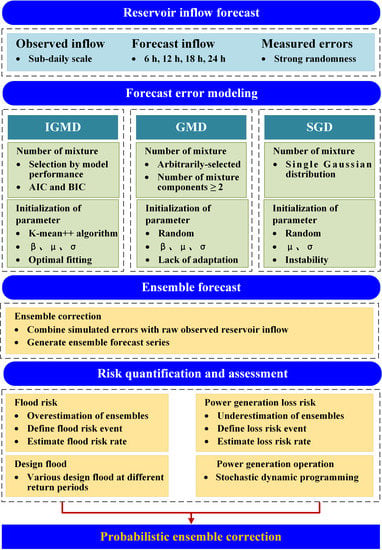
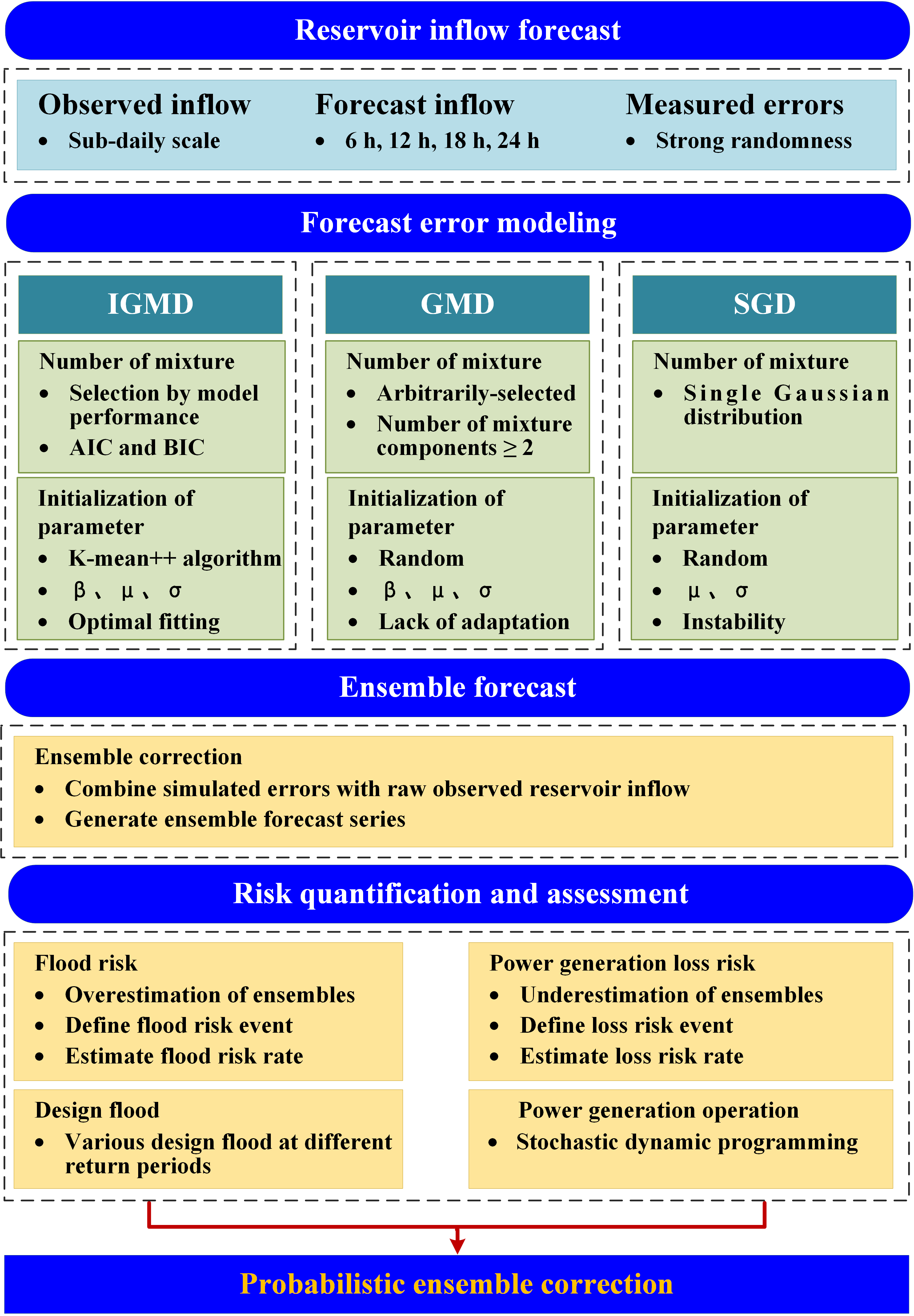
2. Methods
2.1. Gaussian Mixture Distribution (GMD) Model
2.2. Improved Gaussian Mixture Distribution (IGMD) Model
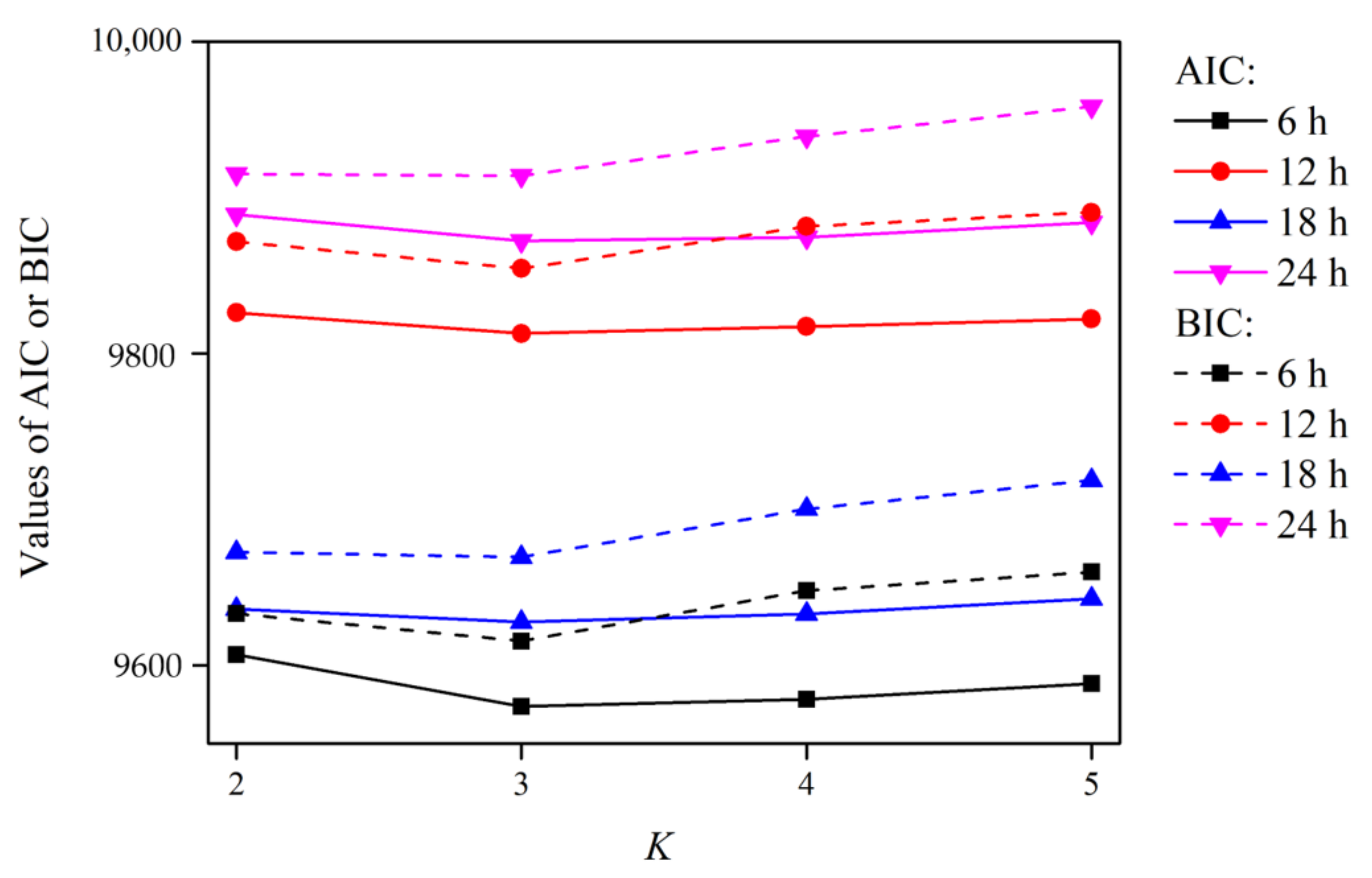
2.2.1. Deciding on the Optimal GMD Models Using the AIC and BIC
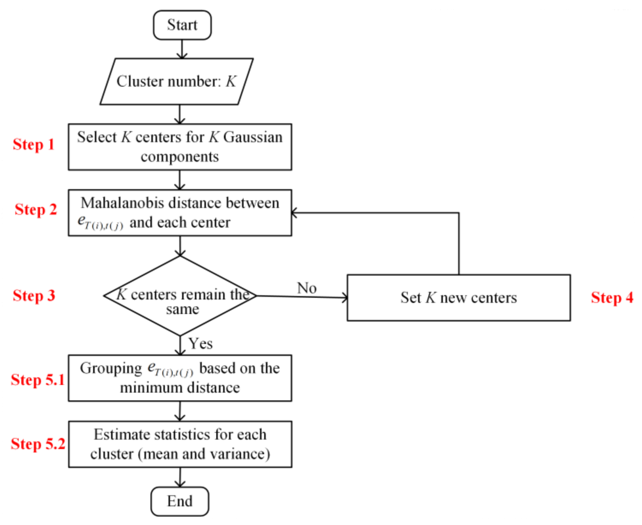
2.2.2. Initializing the Model Parameters Using the k-Mean++ Algorithm
- (a)
- Randomly select K centers for K Gaussian components (K is set to the optimal number quantified in Section 2.2.1) for each sub-daily forecast period.
- (b)
- Estimate the Mahalanobis distance between the forecast error with a lead time of t(j) beginning at time T(i) and the nearest center of the Gaussian model cluster.
- (c)
- Calculate the probability that an error is taken as the next cluster center using the formula , according to the Roulette wheel theory.
- (d)
- Iterate steps (2) and (3) until all the cluster centers remain the same.
- (e)
- Group each error into a specific cluster, where the distance of the error to the center is minimum among K clusters, and derive the cluster mean and variance for each cluster ().
2.2.3. Indices of the Optimal Model Test
2.3. Metropolis–Hastings MCMC Algorithm Based on the IGMD
2.4. Defining a Flood Risk Event Using a Design Flood
2.5. Dynamic Programming Used to Estimate the Electricity Curtailment
3. Study Area and Data
4. Results and Discussion
4.1. Analysis of the IGMD Model
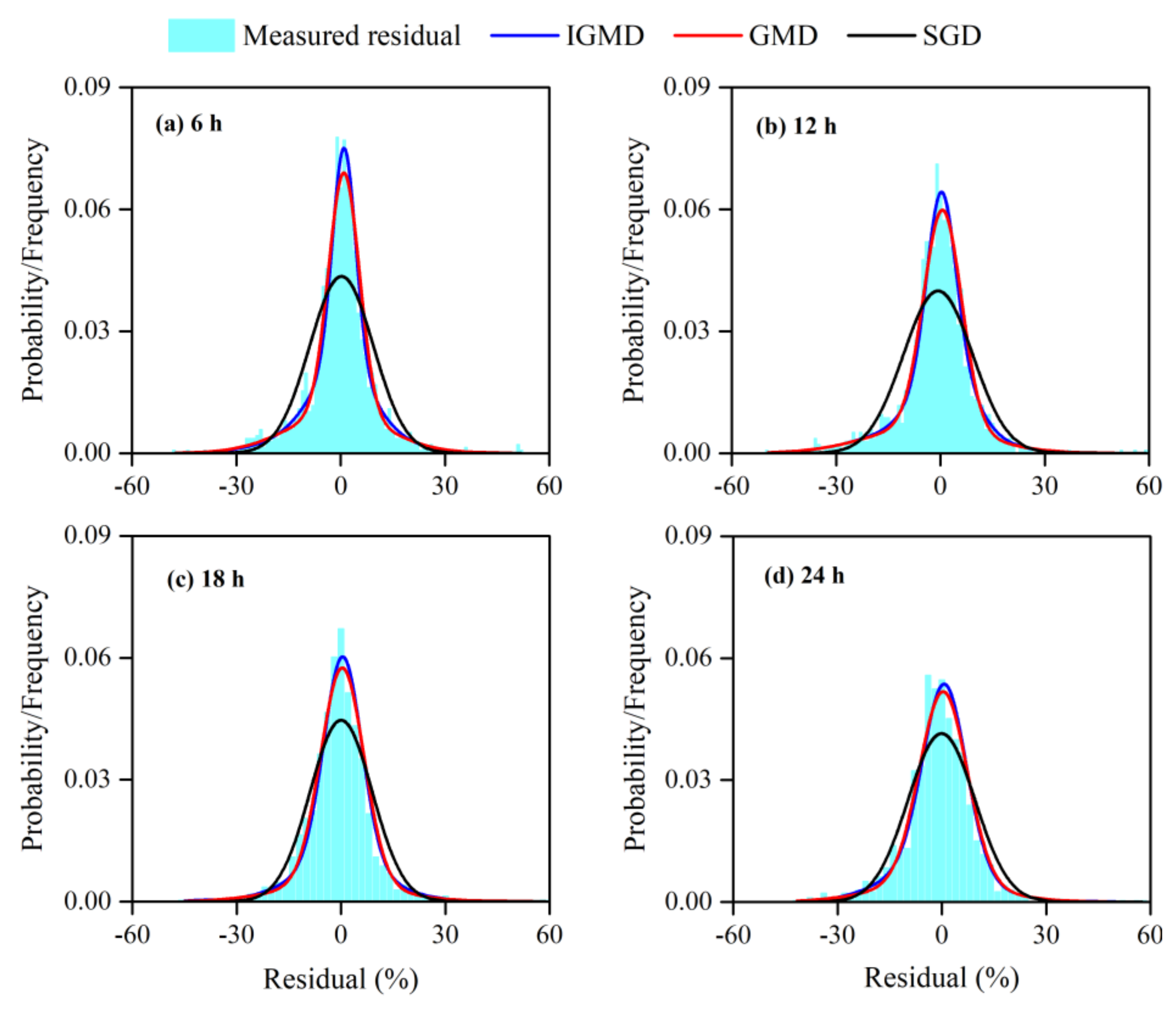
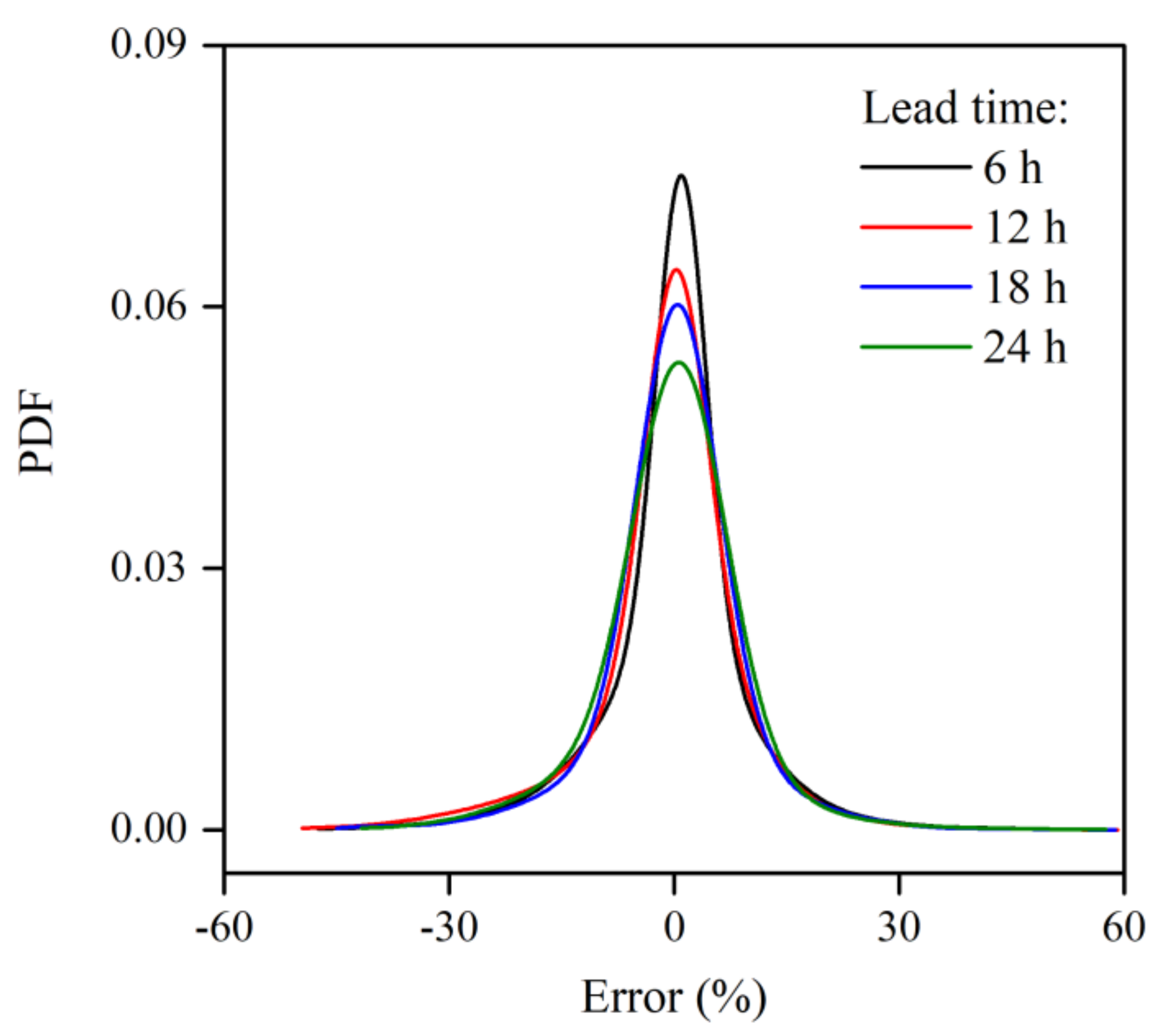
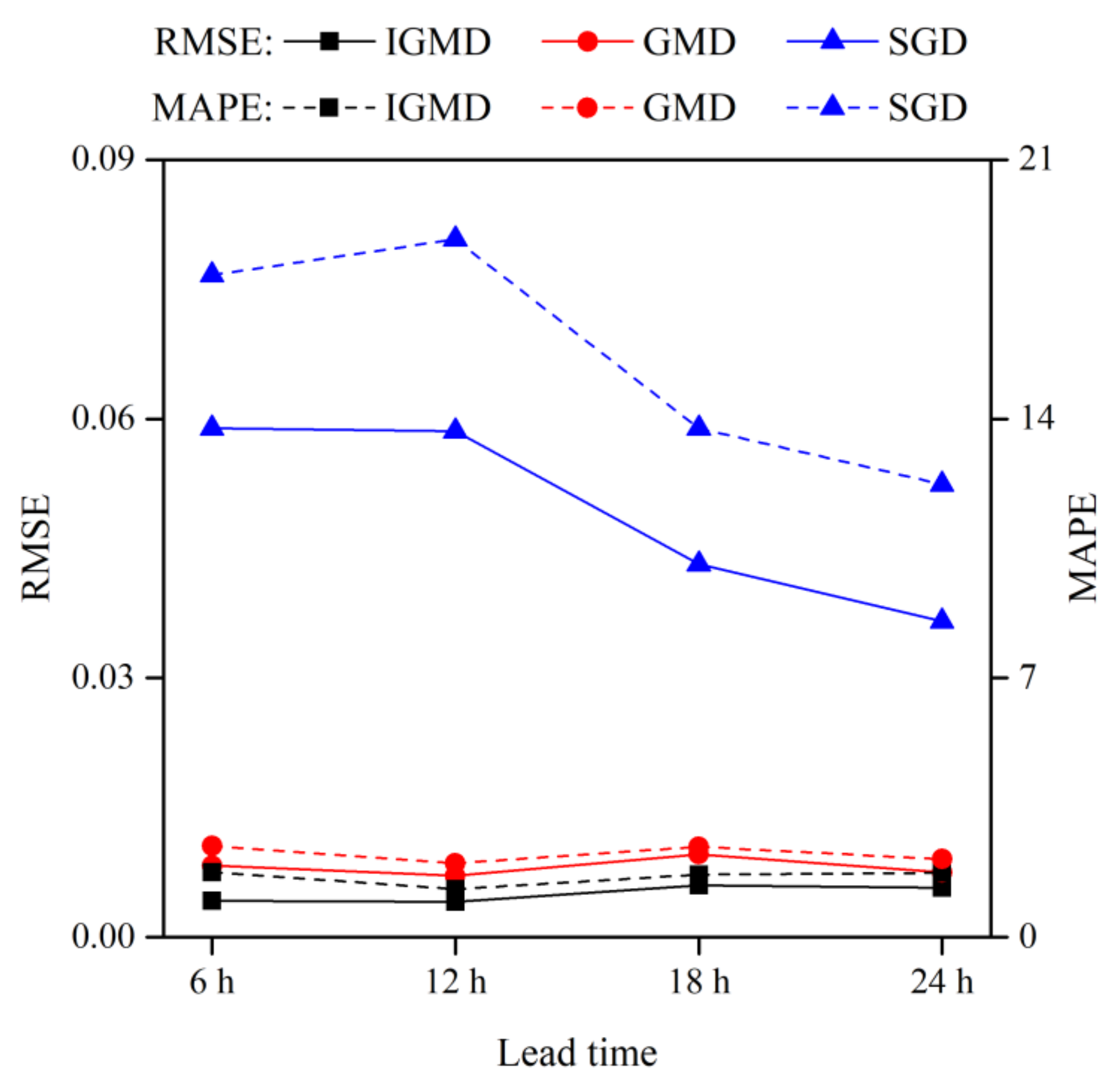
4.1.1. Performance of the IGMD Model
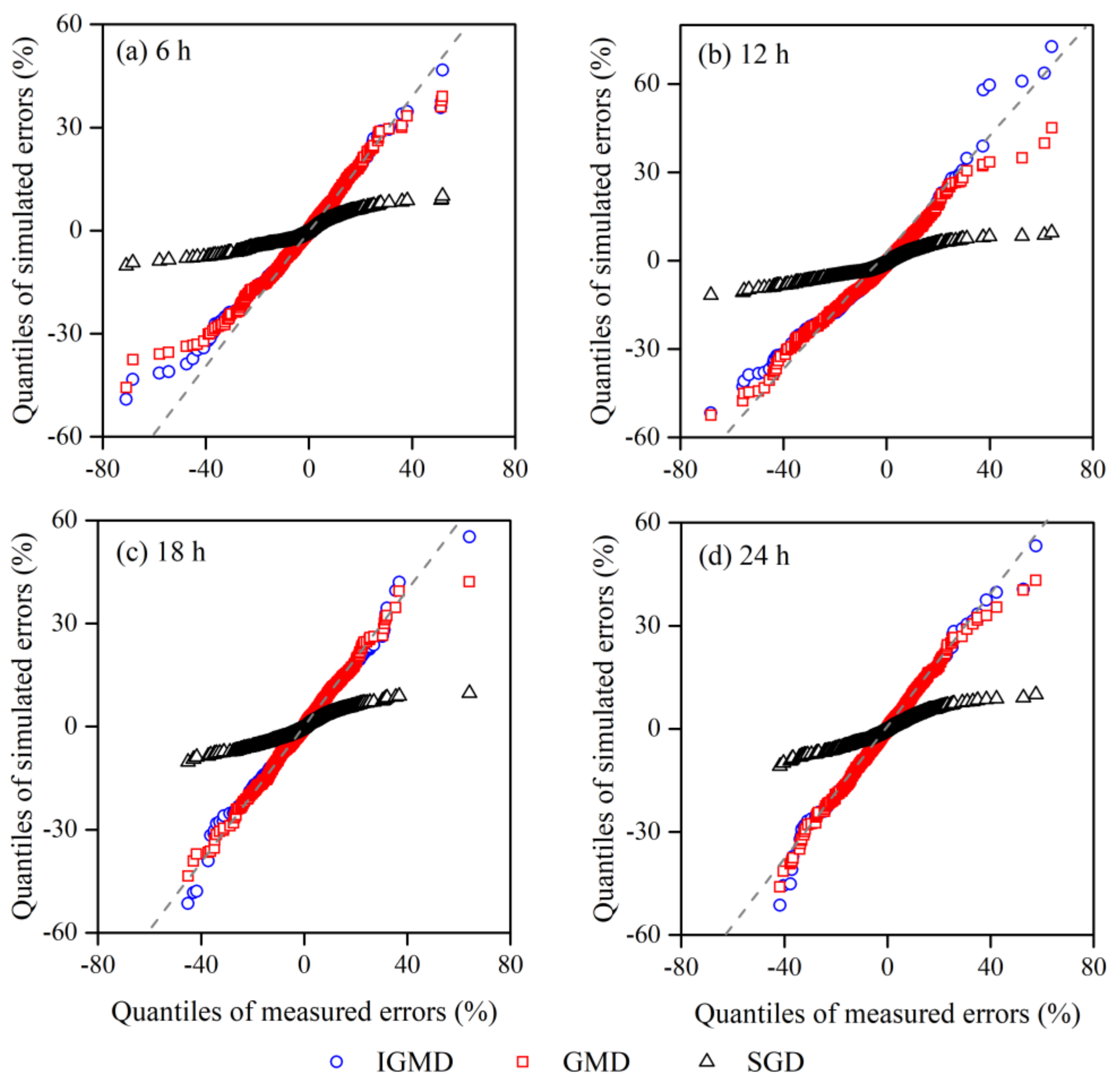
4.1.2. Goodness-of-Fit for the IGMD
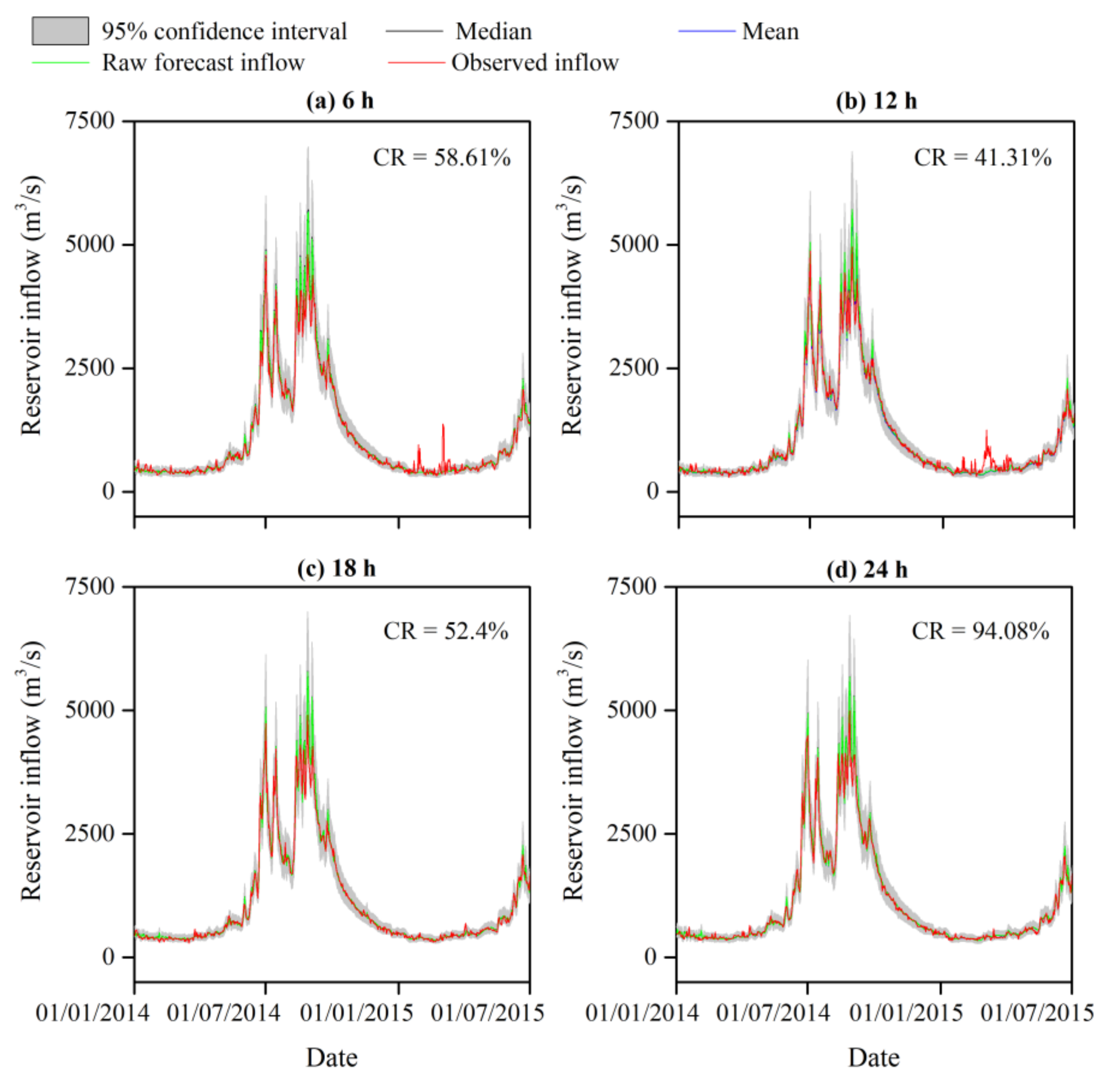
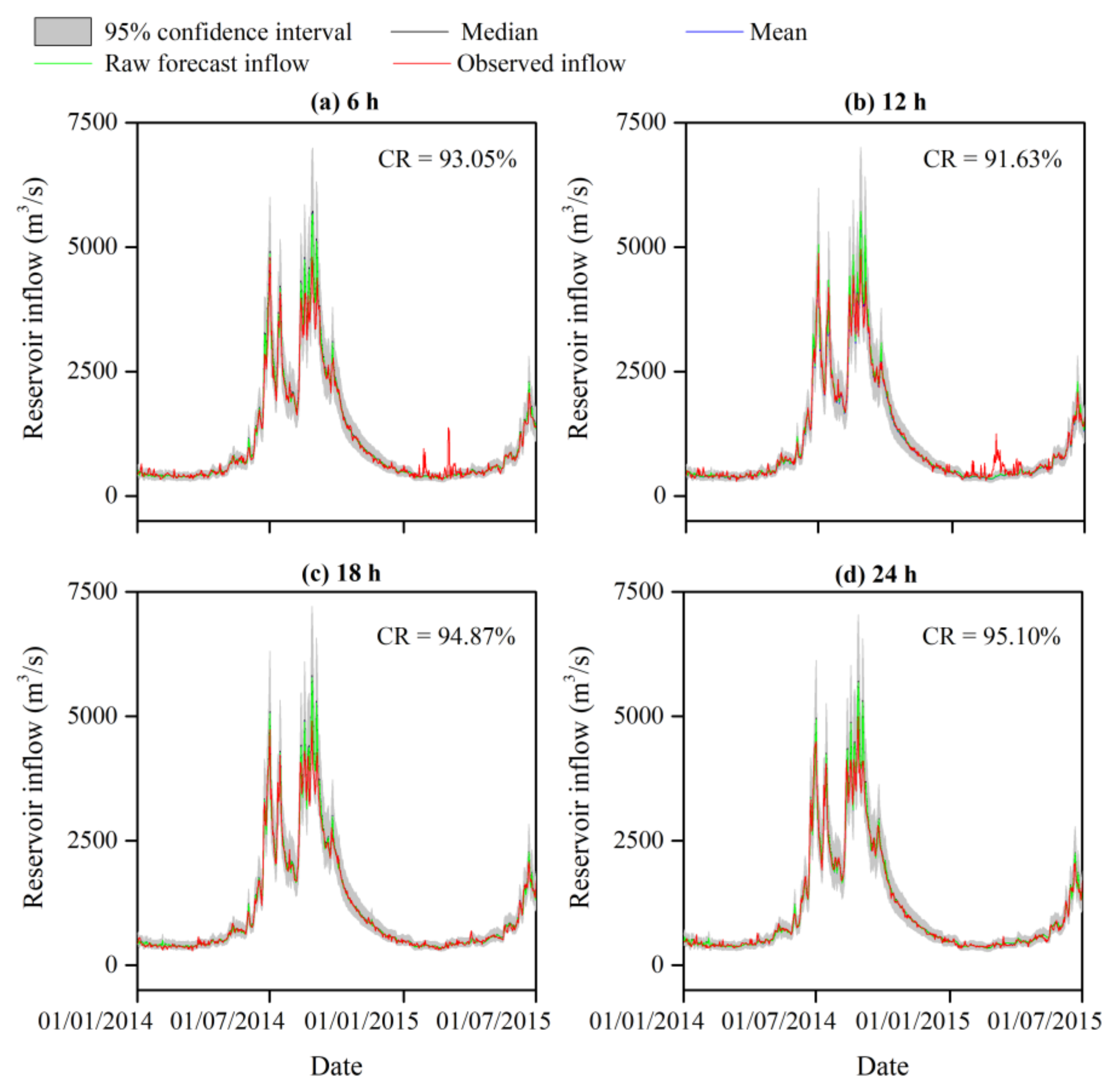
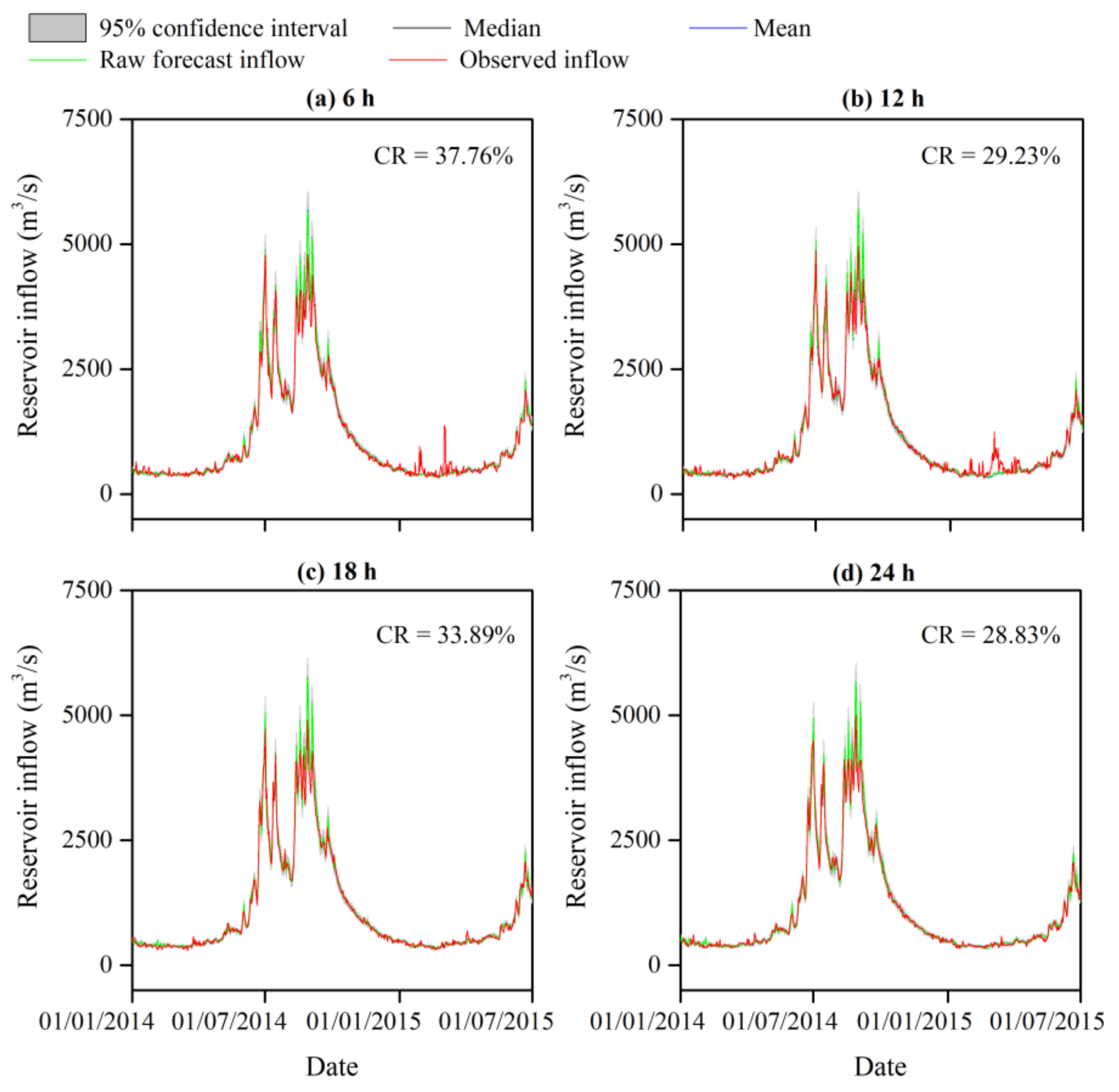
4.2. Uncertainty Analysis of the Reservoir Inflow Forecast
4.3. Risk Assessment from the IFU to the Reservoir Operations
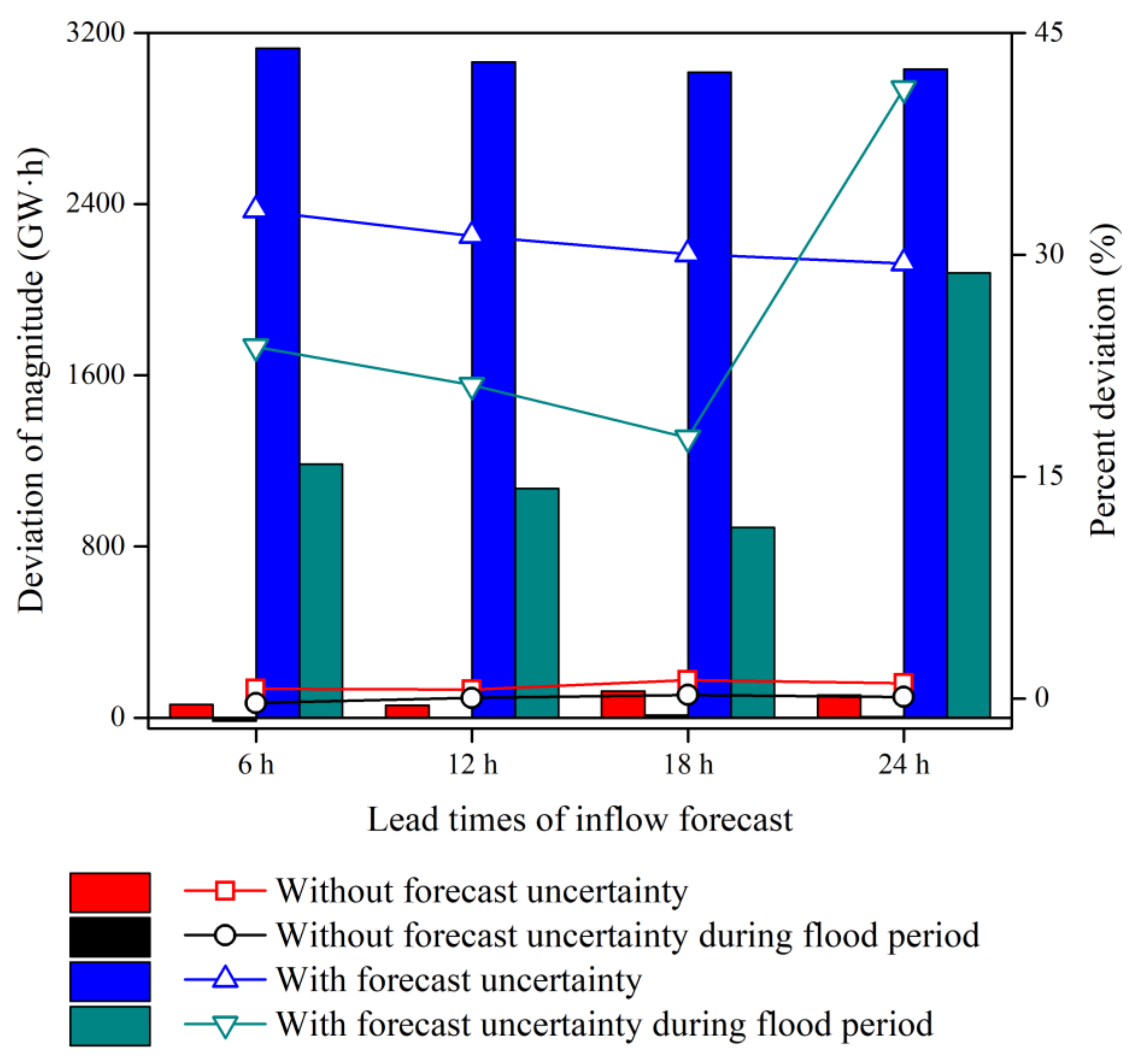
4.3.1. Assessment of the Flood Risk
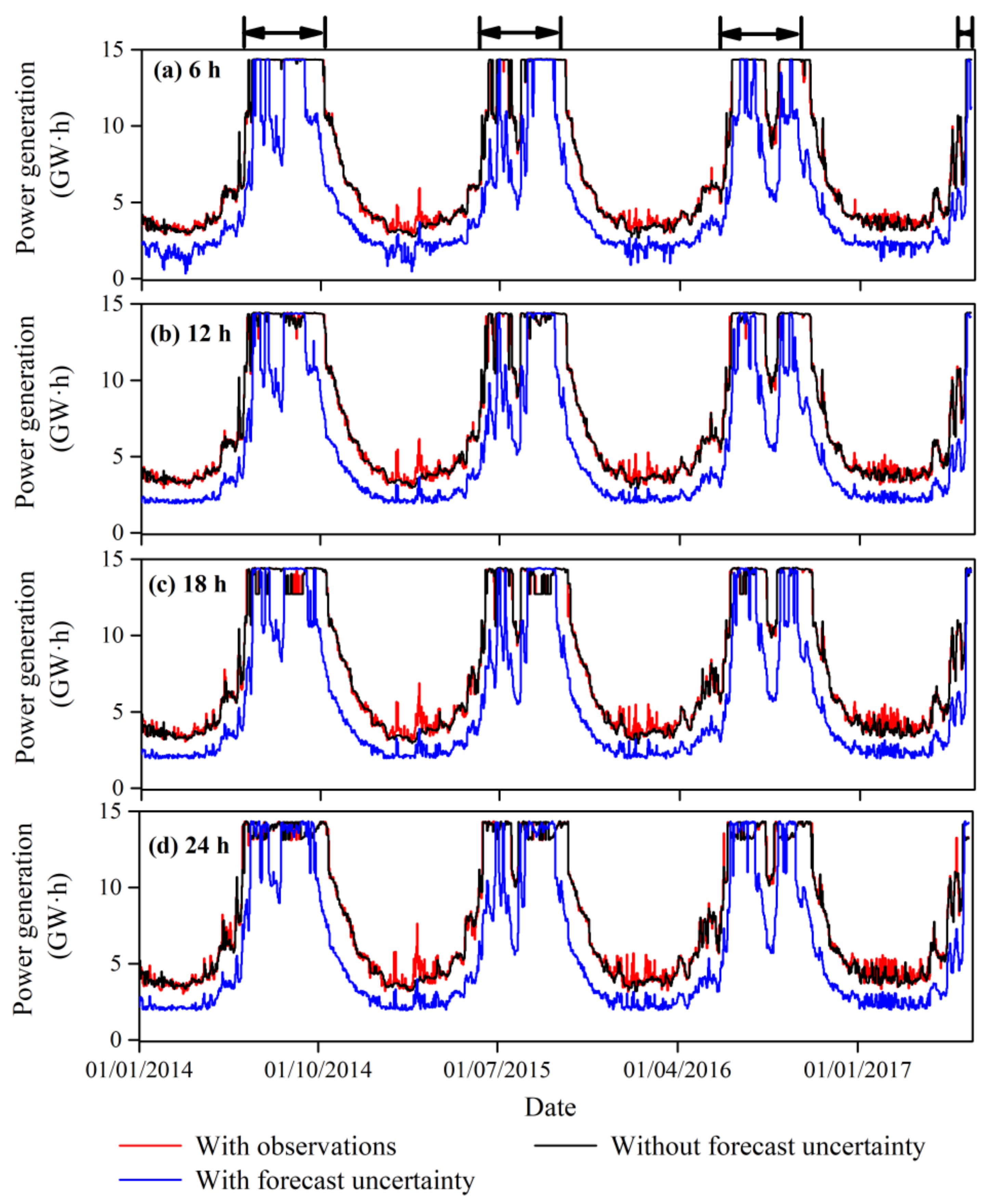
4.3.2. Assessment of the Electricity Curtailment Risk
5. Conclusions
- (1)
- The IGMD model substantially improved the modeling skill of the measured forecast error characteristics and the IGMD-based MCMC algorithm offers a flexible and attractive tool to obtain robust ensemble inflow forecast.
- (2)
- The IGMD-based ensemble approach displayed a high capability of reproducing the observed inflow to support the subsequent reservoir optimal operation and risk assessment, given the limited ensemble size and computational resources.
- (3)
- There existed no flood risk that was defined via the design flood with 10-year and longer return periods when considering the reservoir IFU for each of the sub-daily forecast lead times. In contrast, the electricity curtailment risk significantly increased up to 41%, especially during the non-flood periods, when taking the IFU into account.
Author Contributions
Funding
Institutional Review Board Statement
Informed Consent Statement
Data Availability Statement
Acknowledgments
Conflicts of Interest
References
- Bai, Y.; Chen, Z.; Xie, J.; Li, C. Daily reservoir inflow forecasting using multiscale deep feature learning with hybrid models. J. Hydrol. 2016, 532, 193–206. [Google Scholar] [CrossRef]
- Coulibaly, P.; Anctil, F.; Bobée, B. Daily reservoir inflow forecasting using artificial neural networks with stopped training approach. J. Hydrol. 2000, 230, 244–257. [Google Scholar] [CrossRef]
- Jiang, Z.; Li, R.; Li, A.; Ji, C. Runoff forecast uncertainty considered load adjustment model of cascade hydropower stations and its application. Energy 2018, 158, 693–708. [Google Scholar] [CrossRef]
- Zhou, T.; Liu, Z.; Jin, J.; Hu, H. Assessing the impacts of univariate and bivariate flood frequency approaches to flood risk accounting for reservoir operation. Water 2019, 11, 475. [Google Scholar] [CrossRef] [Green Version]
- Lu, Q.; Zhong, P.; Xu, B.; Zhu, F.; Ma, Y.; Wang, H.; Xu, S. Risk analysis for reservoir flood control operation considering two-dimensional uncertainties based on Bayesian network. J. Hydrol. 2020, 589, 125353. [Google Scholar]
- Winsemius, H.C.; Aerts, J.C.J.H.; Van Beek, L.P.H.; Bierkens, M.F.P.; Bouwman, A.; Jongman, B.; Kwadijk, J.C.J.; Ligtvoet, W.; Lucas, P.L.; Van Vuuren, D.P.; et al. Global drivers of future river flood risk. Nat. Clim. Chang. 2016, 6, 381–385. [Google Scholar] [CrossRef]
- Wasimi, S.A.; Kitanidis, P.K. Real-time forecasting and daily operation of a multireservoir system during floods by linear quadratic Gaussian control. Water Resour. Res. 1983, 19, 1511–1522. [Google Scholar] [CrossRef]
- Chen, L.; Singh, V.P.; Lu, W.; Zhang, J.; Zhou, J.; Guo, S. Streamflow forecast uncertainty evolution and its effect on real-time reservoir operation. J. Hydrol. 2016, 540, 712–726. [Google Scholar] [CrossRef]
- Smith, J.A.; Day, G.N.; Kane, M.D. Nonparametric framework for long-range streamflow forecasting. J. Water Resour. Plan. Manag. 1992, 118, 82–92. [Google Scholar] [CrossRef]
- Liu, X.; Guo, S.; Li, X.; Li, Y. Flood control operation chart for Three Gorges Reservoir considering errors in inflow forecasting. Adv. Water Sci. 2011, 22, 771–779. [Google Scholar]
- Zhao, T.; Cai, X.; Yang, D. Effect of streamflow forecast uncertainty on real-time reservoir operation. Adv. Water Resour. 2011, 34, 495–504. [Google Scholar] [CrossRef]
- Zhao, T.; Zhao, J.; Yang, D.; Wang, H. Generalized martingale model of the uncertainty evolution of streamflow forecasts. Adv. Water Resour. 2013, 57, 41–51. [Google Scholar] [CrossRef]
- Li, X.; Guo, S.; Liu, P.; Chen, G. Dynamic control of flood limited water level for reservoir operation by considering inflow uncertainty. J. Hydrol. 2010, 391, 124–132. [Google Scholar] [CrossRef]
- Zhou, Y.; Guo, S. Risk analysis for flood control operation of seasonal flood-limited water level incorporating inflow forecasting error. Hydrol. Sci. J. 2014, 59, 1006–1019. [Google Scholar] [CrossRef] [Green Version]
- Li, M.; Wang, Q.; Robertson, D.E.; Bennett, J.C. Improved error modelling for streamflow forecasting at hourly time steps by splitting hydrographs into rising and falling limbs. J. Hydrol. 2017, 555, 586–599. [Google Scholar] [CrossRef]
- Li, M.; Wang, Q.J.; Bennett, J.C.; Robertson, D.E. Error reduction and representation in stages (ERRIS) in hydrological modelling for ensemble streamflow forecasting. Hydrol. Earth Syst. Sci. 2016, 20, 3561–3579. [Google Scholar] [CrossRef] [Green Version]
- Ji, C.; Liang, X.; Zhang, Y.; Liu, Y. Stochastic model of reservoir runoff forecast errors and its application. J. Hydroelectr. Eng. 2019, 38, 75–85. [Google Scholar]
- Krzysztofowicz, R. The case for probabilistic forecasting in hydrology. J. Hydrol. 2001, 249, 2–9. [Google Scholar] [CrossRef]
- Xu, X.; Zhang, X.; Fang, H.; Lai, R.; Zhang, Y.; Huang, L.; Liu, X. A real-time probabilistic channel flood-forecasting model based on the Bayesian particle filter approach. Environ. Model. Softw. 2017, 88, 151–167. [Google Scholar] [CrossRef] [Green Version]
- Ma, C.; Cui, X. Rolling forecast for reservoir monthly average flows and its uncertainty. J. Hydroelectr. Eng. 2018, 37, 59–67. [Google Scholar]
- Bourdin, D.R.; Stull, R.B. Bias-corrected short-range Member-to-Member ensemble forecasts of reservoir inflow. J. Hydrol. 2013, 502, 77–88. [Google Scholar] [CrossRef]
- Gournelos, T.; Kotinas, V.; Poulos, S. Fitting a Gaussian mixture model to bivariate distributions of monthly river flows and suspended sediments. J. Hydrol. 2020, 590, 125166. [Google Scholar] [CrossRef]
- Yan, L.; Xiong, L.; Liu, D.; Hu, T.; Xu, C.-Y. Frequency analysis of nonstationary annual maximum flood series using the time-varying two-component mixture distributions. Hydrol. Process. 2017, 31, 69–89. [Google Scholar] [CrossRef]
- Pan, L.; Li, Y.; He, K.; Li, Y.; Li, Y. Generalized linear mixed models with Gaussian mixture random effects: Inference and application. J. Multivar. Anal. 2020, 175, 104555. [Google Scholar]
- Zhuang, X.; Huang, Y.; Palaniappan, K.; Zhao, Y. Gaussian mixture density modeling, decomposition, and applications. IEEE Trans. Image Process. 1996, 5, 1293–1302. [Google Scholar] [CrossRef]
- Chib, S.; Greenberg, E. Understanding the Metropolis-Hastings Algorithm. Am. Stat. 1995, 49, 327. [Google Scholar] [CrossRef]
- Wang, H.; Wang, C.; Wang, Y.; Gao, X.; Yu, C. Bayesian forecasting and uncertainty quantifying of stream flows using Metropolis–Hastings Markov Chain Monte Carlo algorithm. J. Hydrol. 2017, 549, 476–483. [Google Scholar]
- Ma, Q.; Xiong, L.; Liu, D.; Xu, C.-Y.; Guo, S. Evaluating the temporal dynamics of uncertainty contribution from satellite precipitation input in rainfall-runoff modeling using the variance decomposition method. Remote Sens. 2018, 10, 1876. [Google Scholar] [CrossRef] [Green Version]
- Xiong, L.; Wan, M.; Wei, X.; O’Connor, K.M. Indices for assessing the prediction bounds of hydrological models and application by generalised likelihood uncertainty estimation/Indices pour évaluer les bornes de prévision de modèles hydrologiques et mise en œuvre pour une estimation d’incertitude par vraisemblance généralisée. Hydrol. Sci. J. 2009, 54, 852–871. [Google Scholar]
- Li, B.; Liang, Z.; Zhang, J.; Chen, X.; Jiang, X.; Wang, J.; Hu, Y. Risk analysis of reservoir flood routing calculation based on inflow forecast uncertainty. Water 2016, 8, 486. [Google Scholar] [CrossRef] [Green Version]
- Liu, Z.; Lyu, J.; Jia, Z.; Wang, L.-X.; Xu, B. Risks analysis and response of forecast-based operation for Ankang Reservoir flood control. Water 2019, 11, 1134. [Google Scholar] [CrossRef] [Green Version]
- Zeng, X.; Hu, T.; Cai, X.; Zhou, Y.; Wang, X. Improved dynamic programming for parallel reservoir system operation optimization. Adv. Water Resour. 2019, 131, 103373. [Google Scholar] [CrossRef]
- He, S.; Guo, S.; Chen, K.; Deng, L.; Liao, Z.; Xiong, F.; Yin, J. Optimal impoundment operation for cascade reservoirs coupling parallel dynamic programming with importance sampling and successive approximation. Adv. Water Resour. 2019, 131, 103375. [Google Scholar] [CrossRef]
- Wu, S.; Shen, M.; Wang, J. Jinping hydropower project: Main technical issues on engineering geology and rock mechanics. Bull. Eng. Geol. Environ. 2010, 69, 325–332. [Google Scholar]
- Li, M.; Wang, Q.J.; Bennett, J.C.; Robertson, D.E. A strategy to overcome adverse effects of autoregressive updating of streamflow forecasts. Hydrol. Earth Syst. Sci. 2015, 19, 1. [Google Scholar] [CrossRef] [Green Version]


| Model | 6 h | 12 h | 18 h | 24 h |
|---|---|---|---|---|
| IGMD | 0.016 | 0.012 | 0.019 | 0.018 |
| GMD | 0.022 | 0.016 | 0.031 | 0.021 |
| SGD | 0.095 | 0.103 | 0.066 | 0.066 |
| Model | Lead Time | Cv | |||||
|---|---|---|---|---|---|---|---|
| Sampled | Measured | Sampled | Measured | Sampled | Measured | ||
| IGMD | 6 h | 0.238 | 0.236 | 83.575 | 84.081 | 38.489 | 38.838 |
| 12 h | −0.701 | −0.705 | 99.158 | 99.768 | −14.197 | −14.176 | |
| 18 h | 0.027 | 0.025 | 78.873 | 79.837 | 330.079 | 354.592 | |
| 24 h | −0.114 | −0.117 | 91.656 | 92.629 | −84.248 | −82.466 | |
| GMD | 6 h | 0.245 | 0.236 | 83.175 | 84.081 | 37.184 | 38.838 |
| 12 h | −0.675 | −0.705 | 97.642 | 99.768 | −14.632 | −14.176 | |
| 18 h | 0.029 | 0.025 | 76.918 | 79.837 | 304.524 | 354.592 | |
| 24 h | −0.110 | −0.117 | 90.350 | 92.629 | −87.076 | −82.466 | |
| Lead Time | Return Period (year) | Qd (m3/s) | Count(Qem > Qd) | Frequency (%) | Risk Rate (%) |
|---|---|---|---|---|---|
| 6 h | 10,000 | 16,100 | – | – | – |
| 1000 | 13,600 | – | – | – | |
| 100 | 10,900 | – | – | – | |
| 20 | 8850 | – | – | – | |
| 10 | 7920 | – | – | – | |
| 5 | 6920 | – | – | – | |
| 2 | 5390 | 3279 | 32.79 | 16.40 | |
| 12 h | 10,000 | 16,100 | – | – | – |
| 1000 | 13,600 | – | – | – | |
| 100 | 10,900 | – | – | – | |
| 20 | 8850 | – | – | – | |
| 10 | 7920 | – | – | – | |
| 5 | 6920 | – | – | – | |
| 2 | 5390 | 3918 | 39.18 | 19.59 | |
| 18 h | 10,000 | 16,100 | – | – | – |
| 1000 | 13,600 | – | – | – | |
| 100 | 10,900 | – | – | – | |
| 20 | 8850 | – | – | – | |
| 10 | 7920 | – | – | – | |
| 5 | 6920 | 7 | 0.07 | 0.01 | |
| 2 | 5390 | 7966 | 79.66 | 39.83 | |
| 24 h | 10,000 | 16,100 | – | – | – |
| 1000 | 13,600 | – | – | – | |
| 100 | 10,900 | – | – | – | |
| 20 | 8850 | – | – | – | |
| 10 | 7920 | – | – | – | |
| 5 | 6920 | 40 | 0.4 | 0.08 | |
| 2 | 5390 | 9397 | 93.97 | 46.99 |
Publisher’s Note: MDPI stays neutral with regard to jurisdictional claims in published maps and institutional affiliations. |
© 2021 by the authors. Licensee MDPI, Basel, Switzerland. This article is an open access article distributed under the terms and conditions of the Creative Commons Attribution (CC BY) license (http://creativecommons.org/licenses/by/4.0/).
Share and Cite
Ma, Q.; Zhang, J.; Xiong, B.; Zhang, Y.; Ji, C.; Zhou, T. Quantifying the Risks that Propagate from the Inflow Forecast Uncertainty to the Reservoir Operations with Coupled Flood and Electricity Curtailment Risks. Water 2021, 13, 173. https://doi.org/10.3390/w13020173
Ma Q, Zhang J, Xiong B, Zhang Y, Ji C, Zhou T. Quantifying the Risks that Propagate from the Inflow Forecast Uncertainty to the Reservoir Operations with Coupled Flood and Electricity Curtailment Risks. Water. 2021; 13(2):173. https://doi.org/10.3390/w13020173
Chicago/Turabian StyleMa, Qiumei, Jiaxin Zhang, Bin Xiong, Yanke Zhang, Changming Ji, and Ting Zhou. 2021. "Quantifying the Risks that Propagate from the Inflow Forecast Uncertainty to the Reservoir Operations with Coupled Flood and Electricity Curtailment Risks" Water 13, no. 2: 173. https://doi.org/10.3390/w13020173