A Multivariate Balanced Initial Ensemble Generation Approach for an Atmospheric General Circulation Model

Abstract

Based on the multivariate empirical orthogonal function (MEOF) method, a multivariate balanced initial ensemble generation method was applied to the ensemble data assimilation scheme. The initial ensembles were generated with a reasonable consideration of the physical relationships between different model variables. The spatial distribution derived from the MEOF analysis is combined with the 3-D random perturbation to generate a balanced initial perturbation field. The Local Ensemble Transform Kalman Filter (LETKF) data assimilation scheme was established for an atmospheric general circulation model. Ensemble data assimilation experiments using different initial ensemble generation methods, spatially random and MEOF-based balanced, are performed using realistic atmospheric observations. It is shown that the ensembles integrated from the balanced initial ensembles maintain a much more reasonable spread and a more reliable horizontal correlation compared with the historical model results than those from the randomly perturbed initial ensembles. The model predictions were also improved by adopting the MEOF-based balanced initial ensembles.

1. Introduction

The ensemble Kalman filter (EnKF) data assimilation approach was introduced by Evensen in 1994 [1], which is a Monte-Carlo approach and has the potential for efficient use on parallel computers with large-scale geophysical models [2,3,4,5,6,7,8]. The EnKF method uses an ensemble of model forecasts to estimate the background error covariances and optimizes the background with the available observations. So it is easy to implement (no adjoint models are required compared with the three-dimension variational data assimilation [2,9]) and handles strong non-linearities better than other known Kalman filter techniques for large-scale problems [10].

EnKF was first applied to an atmospheric model by Houtekamer and Mitchell [11]. After that, it has rapidly become a promising choice for the operational numerical weather prediction systems. The square root filter (SRF) method of EnKF without perturbed observations (deterministic filters) was proposed by assimilating the observations serially [12,13], and then the EnKF method with perturbed observations (stochastic filters) was applied to a pre-operational system [14]. A local ensemble Kalman filter (LEKF) method that assimilates observations simultaneously was proposed by Ott et al. [15]. Furthermore, the local ensemble transform Kalman filter (LETKF) which uses the ensemble transform Kalman filter (ETKF) approach was proposed to further accelerate LEKF [16,17]. The LETKF assimilates observations within a spatially physical local volume at each model grid point simultaneously and does not require an orthogonal basis which significantly enhances the computational efficiency with parallel implementation [17,18].

For the initial perturbation generation, several kinds of methods have been developed, such as error breeding [19], singular vectors [20], perturbed observations [21] and random perturbations [5,21,22,23]. The performances of these methods were illustrated in several numerical weather prediction models with different complexities [24,25,26,27]. Zheng and Zhu proposed a multivariable empirical orthogonal function (MEOF) based model error perturbation to generate perturbed model errors and then applied it to a global spectral atmospheric model with real observations [28,29]. It should be realized that how to maintain the physical relationships of the different model variables induced by the initial perturbations and how to provide a reasonable background covariance are still an important problem for the ensemble data assimilation process.

In this work, the local ensemble transform Kalman filter approach has been implemented for an atmospheric general circulation model developed by the Institute of Atmospheric Physics (IAP AGCM version 4). A MEOF based balanced perturbation generation method is adopted for generating the initial ensembles, compared with the spatially random perturbation method [5]. The remainder of this paper is structured as follows: In Section 2 and Section 3, the forecast model and the LETKF data assimilation scheme are briefly described respectively. In Section 4, the implementation of the initial perturbation generation scheme based on the multivariate empirical orthogonal function (MEOF) is introduced. In Section 5, the spatially-correlated random perturbation scheme and the MEOF-based balanced perturbation scheme are both applied to the AGCM model results to generate the initial ensemble. The ensemble spread and horizontal correlation of the initial ensembles are compared for the two methods. And the LETKF data assimilation scheme is applied to the AGCM model with the conventional observation data. The characteristics and effects of the random and MEOF based initial ensemble generation methods are illustrated respectively. The data assimilation results using the two different initial ensembles are also shown in this section. Summary and conclusions are drawn in the final section.

2. The Forecast Model

The atmospheric general circulation model used here is the IAP AGCM version 4 as a component of the Chinese Academy of Sciences (CAS) earth system model (ESM). The model was applied to the simulation of atmospheric circulations and climate, such as summer precipitation and monsoons [30,31]. It is a global grid-point model using finite-difference scheme with a terrain-following $\sigma$ coordinate. A latitude-longitude grid with Arakawa’s C grid staggering is used in the horizontal discretization [32,33,34]. The formulation of the governing equations and the finite-difference schemes have several novel features in the IAP AGCM. The model equations are based on the baroclinic primitive equations with subtraction of standard stratification. The purpose of subtracting the standard stratification in the dynamical core is to reduce truncation errors, especially over regions of high terrain. And the IAP model conserves total available energy (sum of kinetic energy, the available potential energy, and the available surface potential energy) rather than total energy. To maintain the conservation of the total available energy, a variable substitution method named the IAP transform is adopted in the numerical design. The model resolution adopted here is 1 degree by 1 degree. The nonlinear iterative time integration method described in [35] is used in the model. The timestep adopted in the numerical simulation here is 1200 seconds. The prognostic model variables are temperature, surface pressure, wind velocity and specific humidity.

3. Data Assimilation Scheme

The Local Ensemble Transform Kalman Filter (LETKF) algorithms used here are based on the work of Hunt et al. [17]. An important advantage of LETKF schemes compared to EnKF is their efficiency in parallel computing. Because LETKF separates the entire global grid into independent local regions, ideally they have the total parallel efficiency [18]. In this section, we introduce the main idea of LETKF briefly.

The ensemble members are defined as $x_i\in {\Re }^n(i=1,\cdots ,N)$, where N is the ensemble size and n is the dimension of the model state. The ensemble matrix X can be constructed by the model states of the ensemble as:

$$X=(x_1,x_2,\cdots ,x_N)\in {\Re }^{n\times N}$$

(1)

The anomaly matrix is

$$X^{\prime }=X-\overline{X}$$

(2)

where $\overline{X}$ is the ensemble mean vector.

To update analysis states at every grid point, the LETKF assimilates only observations within a certain distance from each grid point. Here we use the subscript l to denote a quantity defined on such a local region centered at an analysis grid point. The analysis mean is

$${\overline{x}}_l^a={\overline{x}}_l+x_l{P}_l^a{\left(Y_l\right)}^T{R}_l^{-1}(y_l^o-y_l)$$

(3)

And the analysis error covariance matrix $P_l^a$ is

$$P_l^a={[{(Y_l)}^T{R}_l^{-1}{Y}_l+(N-1)\mathbf{I}/\rho ]}^{-1}$$

(4)

where $R_l$ is the observation error covariance matrix. The observation vector is $y\in {\Re }^m$. $Y=(y_1,\cdots ,y_N)$ and H is the observation operator which interpolates the model state to the observation space. $\rho$ is the multiplicative inflation factor. Within a local region, space localization is carried out by multiplying the inverse observation error covariance matrix with a factor that decays from one to zero as the distance of the observations from the analysis grid point increases [36].

4. Multivariable Balanced Initial Perturbation Scheme

Based on the multivariate empirical orthogonal function MEOF [28], a MEOF-based multivariable initial perturbation method is adopted here to generate a balanced initial ensemble state for the LETKF data assimilation, which can make the ensemble members maintain a reasonable spread as the forecast model integrates. For the MEOF analysis, the snapshots of all the model variables are put in one single vector to make the EOF analysis, instead of making EOF analysis for the model variables individually. The spatial distribution of the model snapshots, which are derived from the MEOF analysis, and the 3-D random perturbation are combined together to generate a balanced perturbation field. The detailed implementation steps of the method are described as follows:

$$Q_i(x,y,z,v)=D(x,y,z,v)+\sum _{j=1}^{N_m}{\sigma }_j(z,v){\varphi }_j(x,y,z,v){\omega }_{i,j},i=1,\cdots ,N$$

(5)

where $Q_i(x,y,z,v)$ represents the generated initial perturbation field for the ith ensemble member, and $D(x,y,z,v)$ represents the initial model state. ${\sigma }_j(z,v)$ represents the standard deviation of model variables in different model layers, which can be calculated from the time coefficients of the MEOF analysis. $N_m$ is the chosen mode number according to the MEOF analysis. ${\varphi }_j(x,y,z,v)$ is the analyzed spatial MEOF mode of the model state variables in different layers. ${\omega }_{i,j}$ is a one-dimension random vector with a mean equal to 0 and variance equal to 1, and the random vectors ${\omega }_{i,j}(j=1,\cdots ,N_m)$ should be independent to make the MEOF modes orthogonal. x, y and z represent the 3-D coordinate, v represents different model variables, and N is the ensemble size.

In practice, we could derive the departures of the model integration results from their average in each model layer first to generate the balanced initial perturbation fields. The standard deviations $\sigma (z,v)$ of the model variables in each model layer could be calculated to normalize the model variables in all the model layers. The MEOF analysis is performed for the normalized model variables and the spatial modes $\varphi (x,y,z,v)$ could be obtained. Finally, we can apply the above equation to generate the initial ensemble perturbation fields. Because the perturbations are a combination of the spatial distribution of all the model variables, the initial ensembles were generated with a reasonable consideration of the physical relationships between different model variables. Then, we can add the derived MEOF based perturbations to the initial state of the model, which are the model’s prognostic variables (i.e., ps, U, V, T, q). After the initial ensembles are generated, we integrate the model for six hours and use the six-hour model forecast as the analysis samples, because it is crucial to check whether the ensemble spread and the spatial correlation at the first analysis time maintain reasonable.

5. Data Assimilation Experiments

Two different initial ensemble generation methods are tested for the LETKF data assimilation of the AGCM. One method is the spatially-correlated random perturbation scheme [5], and the other one is the MEOF-based balanced perturbation scheme. For the two initial perturbation schemes, 80 ensemble members are adopted for the ensemble data assimilation process. The observational data adopted here are the global upper air and surface weather observation data in PREPBUFR format, which are usually used as the conventional observation data for the data assimilation system. The data include land surface, marine surface, radiosonde, pibal and aircraft reports, profiler and radar derived winds, satellite wind data and so on. The data can include pressure, geopotential height, temperature, dew point temperature, wind direction and speed. The conventional observations are grouped into a time window of 6 hours, which are centered on the analysis time, and then are assimilated into the model every 6 hours from 1 January to 10 January 2004, which are at 0000, 0600, 1200 and 1800 UTC. An example figure of the conventional observation data of the surface temperature is shown in Figure 1.

As we can find out in the model integration process, the integration of the temperature variable over time will also influence the integration of the other model variables. So for the generation of the randomly perturbed initial ensemble, we just add a 3-D random noise of a certain magnitude (1% of the magnitude of T) to the temperature variable of the atmosphere general circulation model at all layers, following Evensen’s idea [5]. The random perturbation is generated with a horizontal correlation scale of 2000 km and a vertical correlation scale of 1000 km, as well as a relativity of 0.8 between two adjoint layers. For the generation of the MEOF-based perturbed initial ensemble, we implement the multivariable balanced initial perturbation scheme as described in Section 4. The spatial distribution of the model snapshots derived from the MEOF analysis and the 3-D random perturbation are combined to generate a balanced perturbation field.

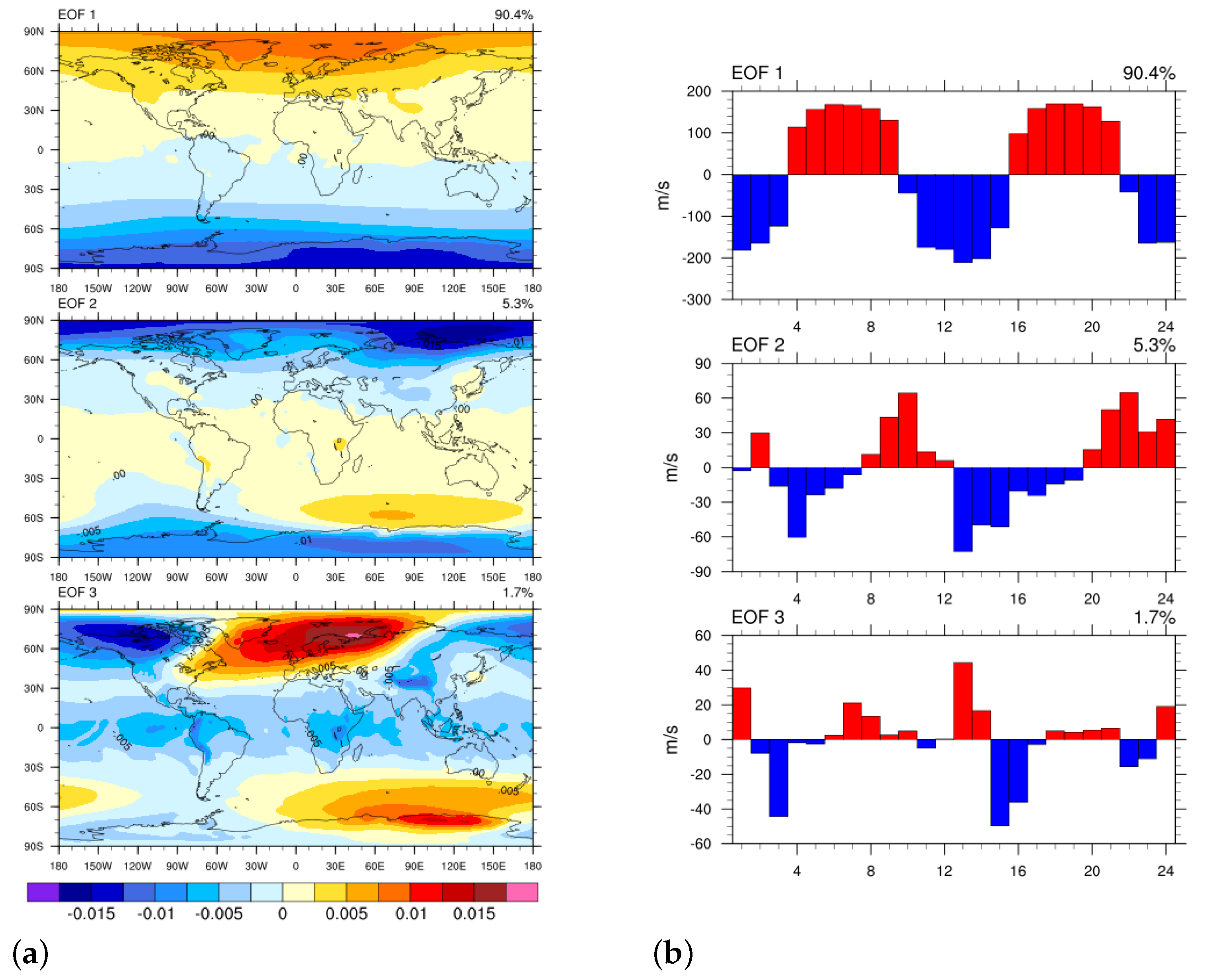
5.1. The MEOF Analysis Results

For the MEOF analysis and the MEOF-based perturbation generation, the AGCM is integrated from 1 January to 31 March 2004 to generate the six-hour model forecast outputs. A total of 360 snapshots are adopted to make the MEOF analysis. Compared to the EOF function analysis for each individual model variable, the MEOF function analysis combines all the model variables in one vector. Figure 2 shows the variance contributions of the first 24 modes for the MEOF analysis of the surface pressure. The total variance contribution of the first 16 MEOF modes have been more than 99%. So the first 20 MEOF modes are adopted to generated the balanced perturbation fields. The spatial distribution and the time coefficients of the first three MEOF modes of the surface pressure (Ps) is shown in Figure 3. Similarly, we can see the detailed MEOF analysis results of the temperature (T) at the surface layer in Figure 4 and Figure 5. The total variance contribution of the first twenty MEOF modes have been also more than 99%.

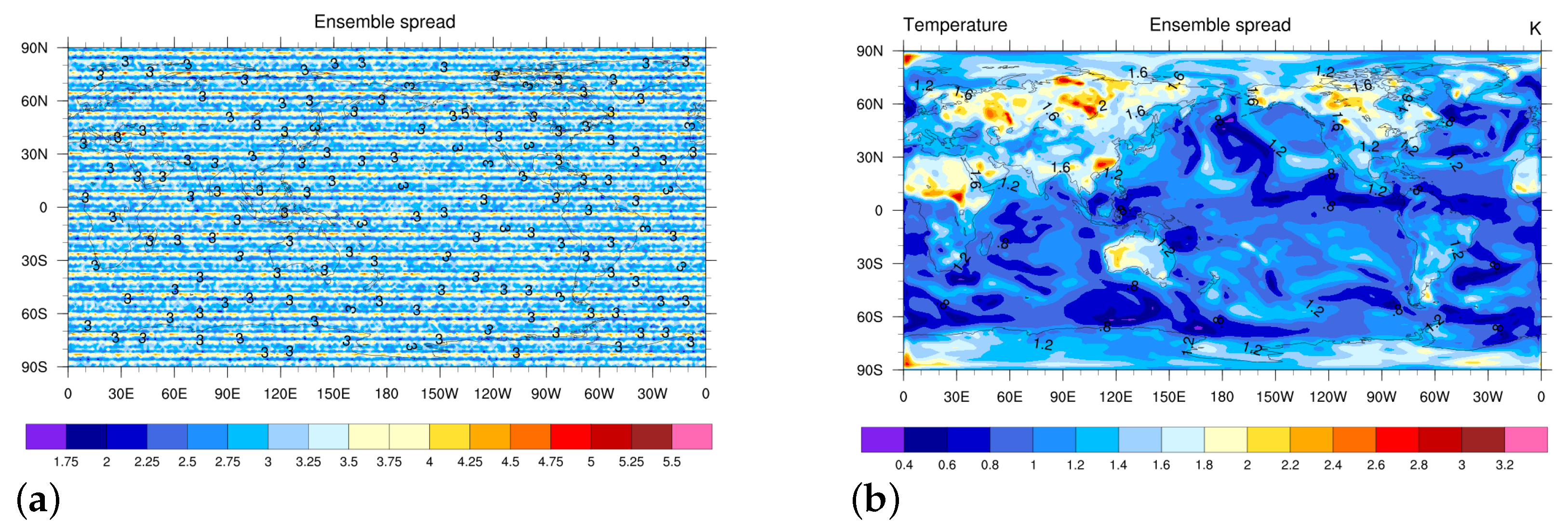
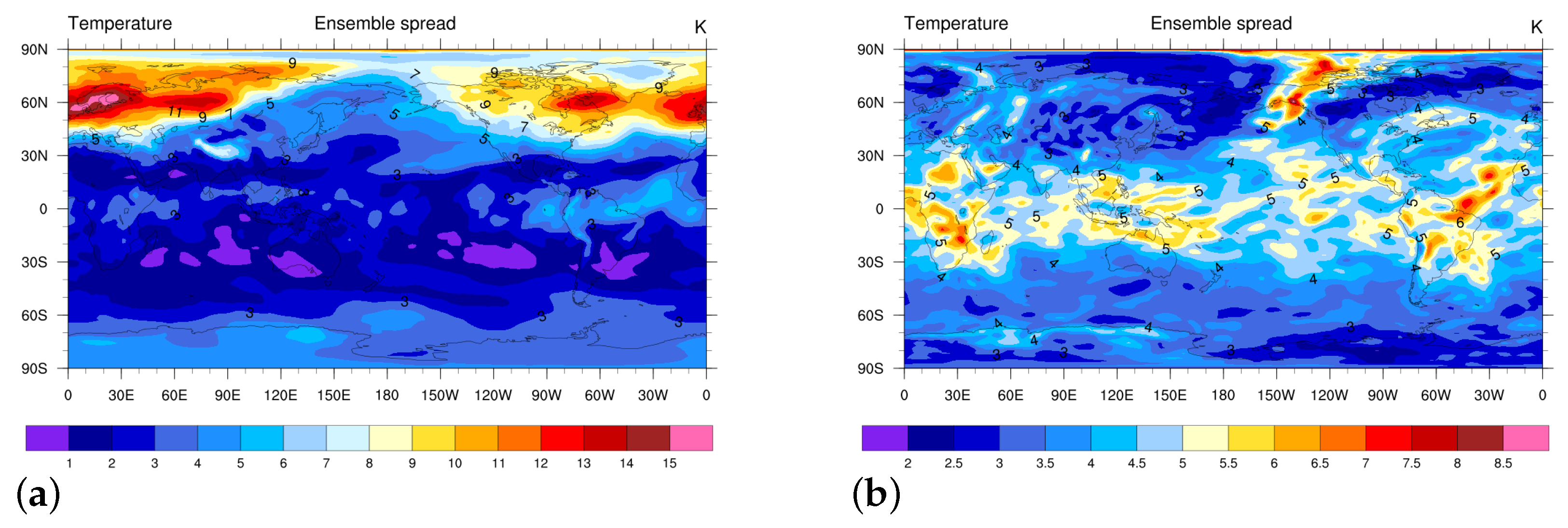
5.2. Ensemble Spread

To verify the quality of the generated initial ensemble, it’s essential to compare the ensemble spread of the initial ensemble and the model outputs after six-hour integration, which is at 06UTC 1 January 2004. A reasonable ensemble spread should represent well the distribution of the forecast uncertainties before the assimilation took place, and a larger ensemble spread can result in a Kalman gain that reasonably draws the analysis closer to the observations [28]. For the random perturbation and the MEOF balanced perturbation scheme, the ensemble spreads of T both decrease after six-hour integration compared with the initial ensemble spread, as shown in Figure 6 and Figure 7. The difference is that the ensemble spread of the MEOF balanced perturbed ensemble decreases much less than that of the randomly perturbed ensemble. The averaged spread of the randomly perturbed initial ensemble of the temperature at the surface layer is about 3.3 degree, which decreases to about 1.4 degree after six-hour integration. As a contrast, the averaged ensemble spread of the MEOF-based balanced initial perturbation of the temperature at the surface layer is about 7.2 degree, which decreases to about 6.1 degree after six-hour integration. It’s shown that the MEOF balanced perturbation could maintain the ensemble spread more reasonable, which is very important for the data assimilation process.

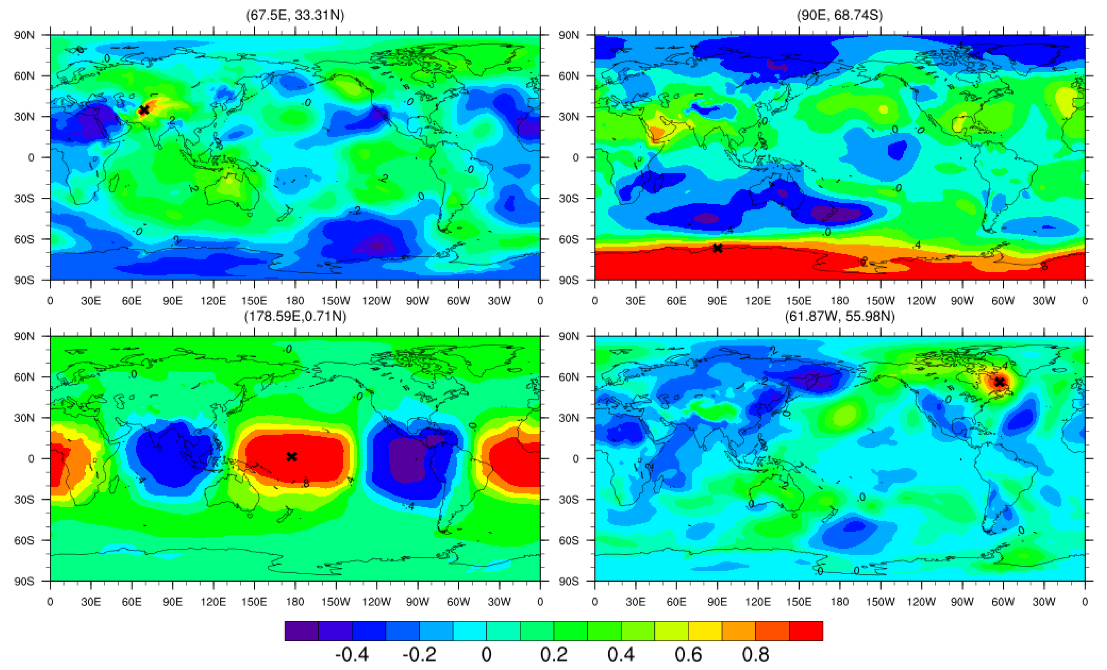
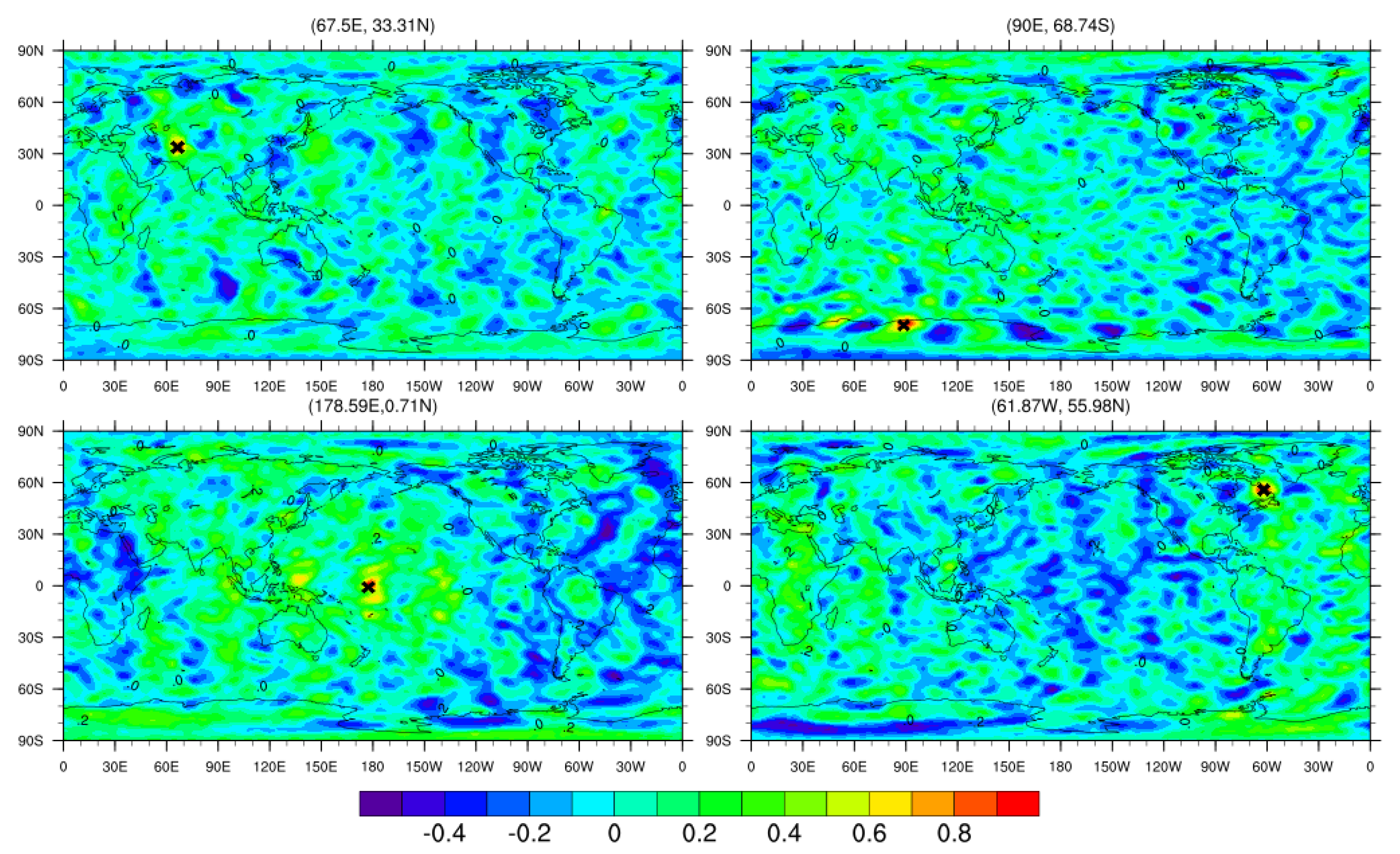
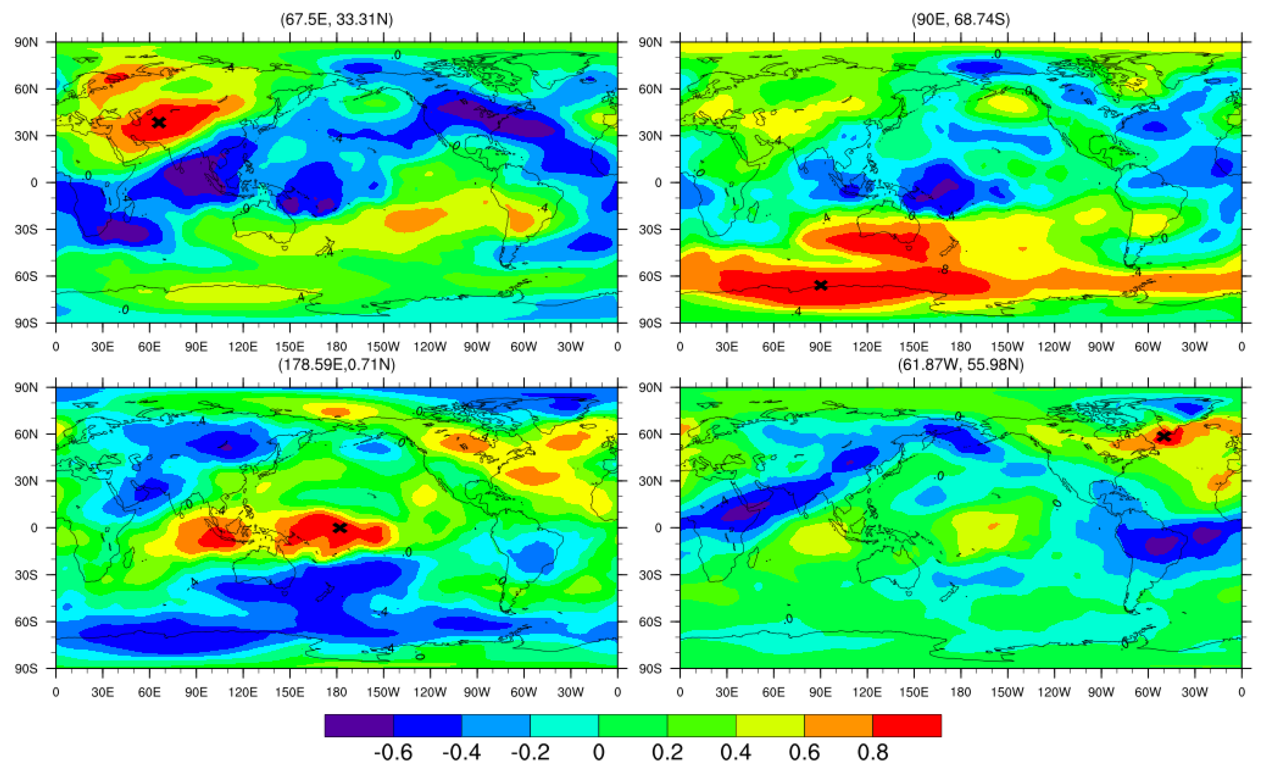
5.3. Horizontal Correlation

Take the surface pressure as example, we calculated the horizontal correlation of four locations for both the randomly perturbed initial ensemble and the MEOF-based balanced initial ensemble. The four locations are chosen as (67.5 E, 33.31 N), (90 E, 68.74 S), (178.59 E, 0.71 S) and (61.87 W, 55.98 N). Figure 8 shows the historical horizontal correlations of the surface pressure at the chosen four locations. The historical results include the six-hour model integration outputs from 1 August to 31 October 2004. Figure 9 shows the horizontal correlations of the randomly perturbed ensemble of the surface pressure at the chosen four locations. The ensembles used to calculate the horizontal correlation is the six-hour forecast of the MEOF-based perturbed initial ensemble. Figure 10 shows the horizontal correlations of the MEOF-based perturbed ensemble of the surface pressure at the chosen four locations. The ensembles used to calculate the horizontal correlation is the six-hour forecast of the randomly perturbed initial ensemble. We can see that the horizontal correlations of the MEOF-based perturbed ensemble of the surface pressure are much more similar to the historical horizontal correlations of the model integration, compared with the horizontal correlations of the randomly perturbed ensemble. The horizontal correlations of the randomly perturbed ensemble have the normal oval shape and can’t represent the historical characteristics in the middle and high latitude area. It’s shown that the ensembles generated from the MEOF perturbations could represent the historical horizontal correlations better. Similar conclusions could be driven for the other state variables, such as the temperature, the wind velocity and humidity.

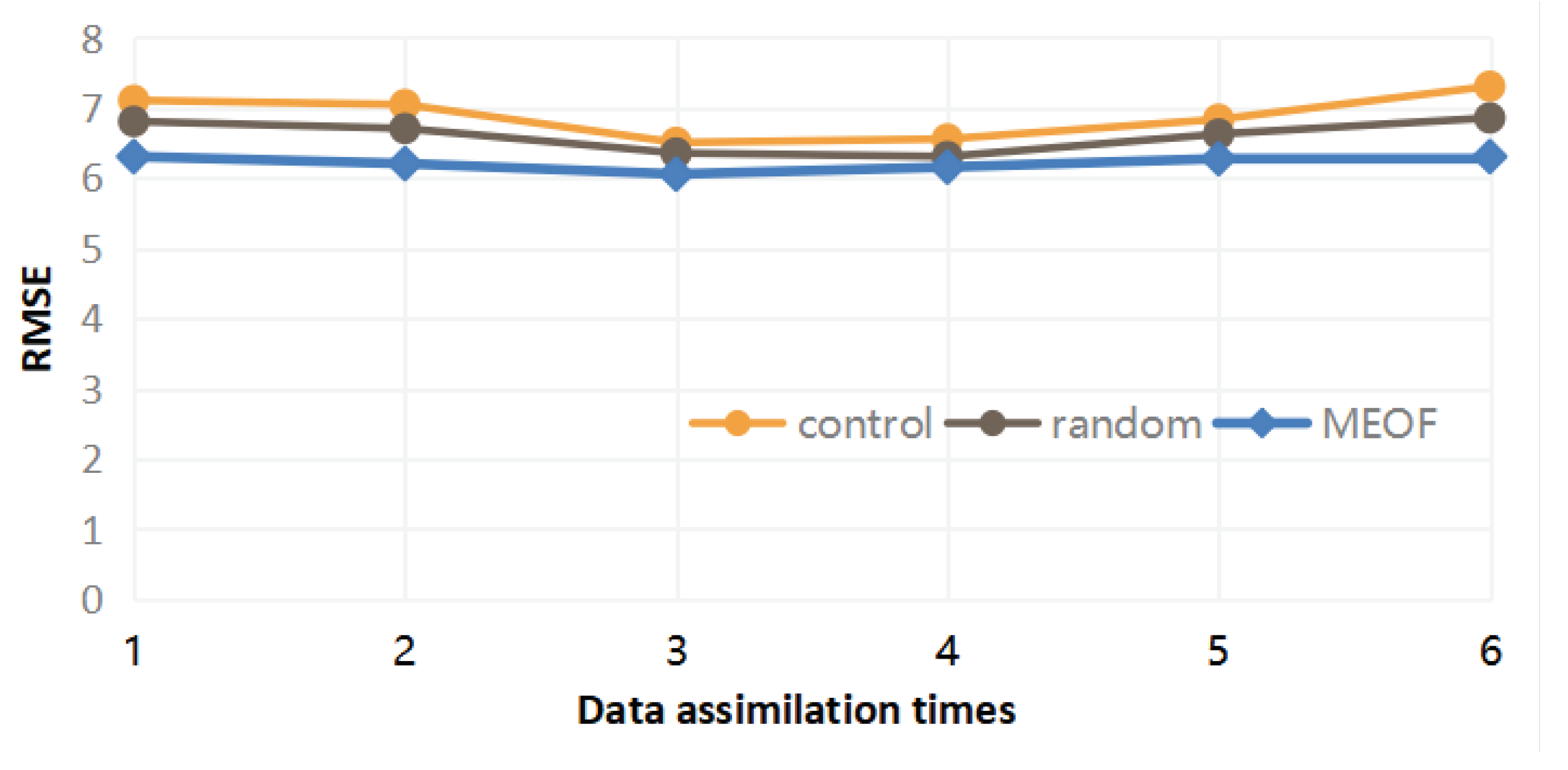
5.4. LETKF Data Assimilation Results

The LETKF data assimilation scheme is applied to the atmospheric general circulation model using 80 ensembles. For the initial ensemble generation, the spatially-correlated random perturbation scheme and the MEOF-based balanced perturbation scheme are implemented and compared from several aspects, such as the ensemble spread and the horizontal correlation. We can see that the initial ensemble generated from the MEOF-based balanced perturbation has a better performance, as the ensemble forecasted from the MEOF-based perturbed initial ensemble could maintain a better spread and their horizontal correlation is more compatible with the horizontal correlation of the historical model output. Here, we adopted the MEOF-based perturbed initial ensemble to start the data assimilation process. The observation adopted here is the six-hour conventional observation data starting from 06UTC 1 January 2004. The observation data of the temperature, the meridional wind and the zonal wind have been assimilated into the AGCM. Figure 11 shows the root mean square error(RMSE) of the LETKF data assimilation results of the surface temperature for the first six data assimilation times, compared with the conventional observation data (see Figure 1). It seems that the RMSE of the data assimilation results derived from both the randomly and MEOF-based perturbed initial ensemble is smaller than the RMSE of the control model, which means the initial ensembles generated from both the two methods worked during the data assimilation process. It’s also shown that the RMSE of the data assimilation results derived from the MEOF-based perturbed initial ensemble is smaller than those derived from the randomly perturbed initial ensemble. Because the initial ensemble generated by the MEOF-based perturbation has better physical relationships between the model variables, the data assimilation effect is further improved. The LETKF data assimilation also improved the meridional and zonal wind result compared to the observation (figures not shown).

6. Conclusions

Based on the multivariate empirical orthogonal function (MEOF) method, a multivariate balanced initial ensemble generation method was applied to the ensemble data assimilation scheme. The initial ensembles were generated with a reasonable consideration of the physical relationships between different model variables. For the initial ensemble generation, the spatially-correlated random perturbation scheme and the MEOF-based balanced perturbation scheme are implemented and compared from several aspects, such as the ensemble spread and the horizontal correlation. From the analysis of ensemble spread and the horizontal correlation, we can see that the initial perturbations generated based on the MEOF method are much more effective considering they will not decay rapidly as the model integrates. The ensembles integrated from the initial ensemble generated from the MEOF-based perturbations will maintain a much more reasonable spread and a more reliable horizontal correlation than those from the randomly perturbed initial fields. The Local Ensemble Transform Kalman Filter (LETKF) data assimilation scheme was established for an atmospheric general circulation model. Ensemble data assimilation experiments using different initial ensemble generation methods, spatially random and MEOF-based balanced, are performed using realistic atmospheric observations. The model predictions were also improved by adopting the MEOF-based balanced multivariate initial ensembles. At the present, only the conventional observation data is assimilated into the AGCM. More data assimilation experiments with the LETKF scheme using the satellite observation data will be made in the future research.

References

1. Evensen, G. Sequential data assimilation with a nonlinear quasi-geostrophic model using Monte Carlo methods to forecast error statistics. J. Geophys. Res. 1994, 99, 10143–10162. [Google Scholar] [CrossRef]
2. Blum, J.; Le Dimet, F.X.; Navon, I.M. Data Assimilation for Geophysical Fluids; Chapter in Computational Methods for the Atmosphere and the Oceans, Volume 14, Special Volume of Handbook of Numerical Analysis; Temam, R., Tribbia, J., Eds.; Elsevier Science Ltd.: New York, NY, USA, 2009; 784p, ISBN 978-0-444-51893-4. [Google Scholar]
3. Burgers, G.; Evensen, G.; Leeuwen, P.J. On the Analysis Scheme in the Ensemble Kalman Filter. Mon. Weather Rev. 1998, 126, 1719–1724. [Google Scholar] [CrossRef]
4. Evensen, G.; Leeuwen, P.J. Assimilation of Geosat Altimeter Data for the Agulhas Current using the Ensemble Kalman Filter with a Quasi-Geostrophic Model. Mon. Weather Rev. 1996, 124, 85–96. [Google Scholar] [CrossRef]
5. Evensen, G. The ensemble Kalman filter: Theoretical formulation and practical implementation. Ocean Dyn. 2003, 53, 343–367. [Google Scholar] [CrossRef]
6. Kalnay, E. Atmospheric Modeling, Data Assimilation and Predictability; Cambridge University Press: London, UK, 2003; 341p. [Google Scholar]
7. Nerger, L.; Hiller, W.; Schroter, J. PDAF—The Parallel Data Assimilation Framework: Experiences with Kalman filtering. In Use of High Performance Computing in Meteorology-Proceedings of the 11 ECMWF Workshop; Zwieflhofer, W., Mozdzynski, G., Eds.; World Scientific: Reading, UK, 2005; pp. 63–83. [Google Scholar]
8. Du, J.; Zhu, J.; Fang, F.; Pain, C.C.; Navon, I.M. Ensemble data assimilation applied to an adaptive mesh ocean model. Int. J. Numer. Meth. Fluids 2016, 82, 997–1009. [Google Scholar] [CrossRef] [Green Version]
9. Du, J.; Navon, I.M.; Zhu, J.; Fang, F.; Alekseev, A.K. Reduced order modeling based on POD of a parabolized Navier-Stokes equations model II: Trust region POD 4D VAR data assimilation. Comput. Math. Appl. 2013, 65, 380–394. [Google Scholar] [CrossRef]
10. Sakov, P.; Oliver, D.S.; Bertino, L. An Iterative EnKF for Strongly Nonlinear Systems. Mon. Weather. Rev. 2011, 140, 1988–2004. [Google Scholar] [CrossRef]
11. Houtekamer, P.L.; Mitchell, H.L. Data assimilation using an ensemble Kalman filter technique. Mon. Wea. Rev. 1998, 126, 796–811. [Google Scholar] [CrossRef]
12. Tippett, M.K.; Anderson, J.L.; Bishop, C.H.; Hamill, T.M.; Whitaker, J.S. Ensemble square root filters. Mon. Wea. Rev. 2003, 131, 1485–1490. [Google Scholar] [CrossRef] [Green Version]
13. Whitaker, J.S.; Hamill, T.M. Ensemble data assimilation without perturbed observations. Mon. Wea. Rev. 2002, 130, 1913–1924. [Google Scholar] [CrossRef]
14. Houtekamer, P.L.; Mitchell, H.L.; Pellerin, G.; Buehner, M.; Charron, M.; Spacek, L.; Hansen, B. Atmospheric data assimilation with an ensemble Kalman filter: Results with real observations. Mon. Wea. Rev. 2005, 133, 604–620. [Google Scholar] [CrossRef] [Green Version]
15. Ott, E.; Hunt, B.R.; Szunyogh, I.; Zimin, A.V.; Kostelich, E.J.; Corazza, M.; Kalnay, E.; Patil, D.J.; Yorke, J.A. A local ensemble Kalman filter for atmospheric data assimilation. Tellus 2004, 56, 415–428. [Google Scholar] [CrossRef]
16. Bishop, C.H.; Etherton, B.; Majumdar, S.J. Adaptive sampling with the ensemble transform Kalman filter. Part I: Theoretical aspects. Mon. Wea. Rev. 2001, 129, 420–436. [Google Scholar] [CrossRef]
17. Hunt, B.; Kostelich, E.; Syzunogh, I. Efficient data assimilation for spatiotemporal chaos: A local ensemble transform Kalman filter. Physica D 2007, 230, 112–126. [Google Scholar] [CrossRef] [Green Version]
18. Miyoshi, T.; Yamane, S. Local ensemble transform Kalman filtering with an agcm at a T159/L48 resolution. Mon. Wea. Rev. 2007, 135, 3841–3861. [Google Scholar] [CrossRef] [Green Version]
19. Toth, Z.; Kalnay, E. Ensemble forecasting at NCEP and the breeding method. Mon. Wea. Rev. 1997, 125, 3297–3319. [Google Scholar] [CrossRef]
20. Buizza, R.; Palmer, T.N. The singular-vector structure of the atmospheric global circulation. J. Atmos. Sci. 1995, 52, 1434–1456. [Google Scholar] [CrossRef] [Green Version]
21. Houtekamer, P.L.; Derome, J. Methods for ensemble prediction. Mon. Wea. Rev. 1995, 123, 2181–2196. [Google Scholar] [CrossRef] [Green Version]
22. Du, J.; Mullen, S.L.; Sanders, F. Short-range ensemble forecasting of quantitative precipitation. Mon. Wea. Rev. 1997, 125, 2427–2459. [Google Scholar] [CrossRef]
23. Wan, L.; Zhu, J.; Bertino, L.; Wang, H. Initial ensemble generation and validation for ocean data assimilation using HYCOM in the Pacific. Ocean Dyn. 2008, 58, 81–99. [Google Scholar] [CrossRef]
24. Hamill, T.M.; Snyder, C.; Morss, R.E. A comparison of probabilistic forecasts from bred, singular-vector, and perturbed observation ensembles. Mon. Wea. Rev. 2000, 128, 1835–1851. [Google Scholar] [CrossRef]
25. Magnusson, L.; Nycander, J.; Kallen, E. Flow-dependent versus flow-independent initial perturbations for ensemble prediction. Tellus 2009, 61A, 194–209. [Google Scholar] [CrossRef] [Green Version]
26. Wang, X.; Bishop, C.H. A comparison of breeding and ensemble transform Kalman filter ensemble forecast schemes. J. Atmos. Sci. 2003, 60, 1140–1158. [Google Scholar] [CrossRef]
27. Zupanski, M.; Fletcher, S.J.; Navon, I.M.; Uzunoglu, B.; Daescu, D. Initiation of ensemble data assimilation. Tellus 2006, 58A, 159–170. [Google Scholar] [CrossRef] [Green Version]
28. Zheng, F.; Zhu, J. Balanced multivariate model errors of an intermediate coupled model for ensemble Kalman filter data assimilation. J. Geophys. Res. 2008, 113, C07002. [Google Scholar] [CrossRef] [Green Version]
29. Zheng, F.; Zhu, J. A multivariate empirical orthogonal function-based scheme for the balanced initial ensemble generation of an ensemble kalman filter. Atmos. Ocean. Sci. Lett. 2010, 3, 165–169. [Google Scholar]
30. Lin, Z.; Zeng, Q. Simulation of East Asian summer monsoon by using an improved AGCM. Adv. Atmos. Sci. 1997, 14, 513–526. [Google Scholar]
31. Zeng, Q.; Yuan, C.; Li, X.; Zhang, R.; Yang, F.; Zhang, B.; Lu, P.; Bi, X.; Wang, H. Seasonal and extraseasonal predictions of summer monsoon precipitation by GCMs. Adv. Atmos. Sci. 1997, 14, 163–176. [Google Scholar]
32. Zeng, Q.; Zhang, X.H.; Liang, X.Z.; Yuan, C.G.; Chen, S.F. Documentation of IAP Two-Level Atmospheric General Circulation Model; Rep. DOE/ER/60314-H1 TR044; Department of Energy Tech., State Univ. of New York: Stony Brook, NY, USA, 1989; 383p. [Google Scholar]
33. Zhang, H.; Zhang, M.; Zeng, Q. Sensitivity of simulated climate to two atmospheric models: Interpretation of differences between dry models and moist models. Mon. Weather. Rev. 2013, 141, 1558–1576. [Google Scholar] [CrossRef]
34. Zhang, H. Development of IAP Atmospheric General Circulation Model Version 4.0 and Its Climate Simulations (in Chinese). Ph.D. Thesis, Institute of Atmospheric Physics, Chinese Academy of Sciences, Beijing, China, 2009. [Google Scholar]
35. Zuo, R.; Zhang, M.; Zhang, D.; Wang, A.; Zeng, Q. Designing and climatic numerical modeling of 21-level AGCM (IAP AGCM-III). Part I: Dynamical framework (in Chinese). Chin. Atmos. Sci. 2004, 28, 659–674. [Google Scholar]
36. Shin, S.; Kang, J.S.; Jo, Y. The Local Ensemble Transform Kalman Filter (LETKF) with a Global NWP Model on the Cubed Sphere. Pure Appl. Geophys. 2016, 173, 2555–2570. [Google Scholar] [CrossRef] [Green Version]
Figure 1. Conventional observation data of temperature at the surface layer at 06UTC 20040101.
Water 13 00122 g001
Figure 2. Variance contributions of the first 24 modes from the MEOF analysis of Ps.
Water 13 00122 g002
Figure 3. The spatial distribution (a) and the time coefficients (b) of the first three modes of the MEOF analysis of Ps.
Water 13 00122 g003
Figure 4. Variance contributions of the first 24 modes from the MEOF analysis of T.
Water 13 00122 g004
Figure 5. The spatial distribution (a) and the time coefficients (b) of the first three modes of the MEOF analysis of T.
Water 13 00122 g005
Figure 6. The initial (a) and the 6-h integration (b) ensemble spread of the randomly perturbed T.
Water 13 00122 g006
Figure 7. The initial (a) and the 6-h integration (b) ensemble spread of the MEOF perturbed T.
Water 13 00122 g007
Figure 8. The historical horizontal correlation of the model integration results at four locations.
Water 13 00122 g008
Figure 9. The horizontal correlation of the randomly perturbed ensemble at four locations.
Water 13 00122 g009
Figure 10. The horizontal correlation of the MEOF based perturbed ensemble at four locations.
Water 13 00122 g010
Figure 11. The RMSE of the LETKF data assimilation results compared with the observation data for the surface temperature.
Water 13 00122 g011
Publisher’s Note: MDPI stays neutral with regard to jurisdictional claims in published maps and institutional affiliations.