
Soil Moisture and Salinity Inversion Based on New Remote Sensing Index and Neural Network at a Salina-Alkaline Wetland


1
School of Ecology and Environment, Inner Mongolia University, Hohhot 010021, China
2
Inner Mongolia Key Laboratory of River and Lake Ecology, Hohhot 010021, China
*
Author to whom correspondence should be addressed.
Water 2021, 13(19), 2762; https://doi.org/10.3390/w13192762
Submission received: 16 August 2021
/
Revised: 21 September 2021
/
Accepted: 25 September 2021
/
Published: 6 October 2021
(This article belongs to the Special Issue Soil Hydrological Processes in Desert Regions)
Abstract
:In arid and semi-arid regions, soil moisture and salinity are important elements to control regional ecology and climate, vegetation growth and land function. Soil moisture and salt content are more important in arid wetlands. The Ebinur Lake wetland is an important part of the ecological barrier of Junggar Basin in Xinjiang, China. The Ebinur Lake Basin is a representative area of the arid climate and ecological degradation in central Asia. It is of great significance to study the spatial distribution of soil moisture and salinity and its causes for land and wetland ecological restoration in the Ebinur Lake Basin. Based on the field measurement and Landsat 8 satellite data, a variety of remote sensing indexes related to soil moisture and salinity were tested and compared, and the prediction models of soil moisture and salinity were established, and the accuracy of the models was assessed. Among them, the salinity indexes D1 and D2 were the latest ones that we proposed according to the research area and data. The distribution maps of soil moisture and salinity in the Ebinur Lake Basin were retrieved from remote sensing data, and the correlation analysis between soil moisture and salinity was performed. Among several soil moisture and salinity prediction indexes, the normalized moisture index NDWI had the highest correlation with soil moisture, and the salinity index D2 had the highest correlation with soil salinity, reaching 0.600 and 0.637, respectively. The accuracy of the BP neural network model for estimating soil salinity was higher than the one of other models; R2 = 0.624, RMSE = 0.083 S/m. The effect of the cubic function prediction model for estimating soil moisture was also higher than that of the BP neural network, support vector machine and other models; R2 = 0.538, RMSE = 0.230. The regularity of soil moisture and salinity changes seemed to be consistent, the correlation degree was 0.817, and the synchronous change degree was higher. The soil salinity in the Ebinur Lake Basin was generally low in the surrounding area, high in the middle area, high in the lake area and low in the vegetation coverage area. The soil moisture in the Ebinur Lake Basin slightly decreased outward with the Ebinur Lake as the center and was higher in the west and lower in the east. However, the spatial distribution of soil moisture had a higher mutation rate and stronger heterogeneity than that of soil salinity.
1. Introduction
Wetlands play an important role in the global ecosystem. Wetlands are easy to degrade, and their shrinkage is more obvious in arid areas. Wetlands, as an important carrier of water resources in arid areas, have irreplaceable ecological functions. In an arid area, wetlands are very sensitive to changes in soil environmental factors. In arid and semi-arid areas, changes in soil physical and chemical properties may lead to changes in wetland ecology and climate [1]. Especially in arid and semi-arid areas, the changes in soil physical and chemical properties may lead to regional ecological and climate change. Comprehensive stress of soil moisture and salinity is one of the principal factors that restrict wetland restoration in arid and semi-arid areas [2]. For example, soil salinization exerts a strong stress on the wetland and its surrounding vegetation, which leads to blocked vegetation growth and land degradation to a certain extent, and may lead to abnormal succession of ecological community, ultimately leading to the decline of wetland ecological function and productivity [3,4]. Soil moisture is used to measure available water in the soil. Soil moisture stress can result in serious desertification, degradation of vegetation productivity and change of regional microclimate in waterless areas [5]. Therefore, it is of great significance to accurately grasp the spatial distribution and formation of soil water and salt in arid and semi-arid areas for controlling natural disasters, such as land desertification and drought, as well as for protecting and restoring wetlands in arid and semi-arid areas.
In order to obtain detailed information of soil moisture and salinity distribution, traditional measurements of soil properties require large numbers of experimental samples, long-term observation of soil characteristics and surrounding vegetation information as support, which requires a huge amount of manpower, financial resources and time [6] and is not suitable for long-term monitoring due to the influence of weather. For example, in the case of bad weather conditions (rainstorm, strong wind, etc.), the field survey work of field surveyors is greatly hindered. Therefore, remote sensing has become an ideal technology for identifying, monitoring and successfully retrieving soil moisture and salinity content with its unique advantages of macroscopic, comprehensive, fast information acquisition, short cycle and dynamic reflection of the changes on the ground [7]. Soil moisture is usually retrieved by optical remote sensing or microwave remote sensing. In optical remote sensing, the common method includes using Landsat, IKONOS or MODIS multi-spectral data to establish the corresponding water index, drought index or vegetation index (such as the most commonly used vegetation index—the normalized vegetation index, NDVI [8,9]) to extract soil moisture [10,11,12]. It also contains the use of surface temperature or thermal inertia to realize soil moisture inversion [13]. Sinha et al. studied the emission characteristics of visible and near infrared spectra of alluvial soil, red loam and black cotton soil, and found that the three soils under different conditions were negatively correlated with soil moisture [14]. At the same time, some researchers have carried out studies on soil moisture and soil multispectral characteristics, indicating that visible, mid-infrared and near-infrared lights are significantly correlated with soil moisture [15]. Comparatively, spectral data in the mid-infrared band have the highest correlation with soil moisture, indicating the best effect. Ghulam et al. proposed the modified vertical drought index (MPDI) to monitor soil water content by analyzing the spectral characteristic space of soil water and found that although MPDI had a good monitoring effect, its application scope was limited [16]. Subsequently, Zhang et al. proposed a new index, RDMI, to monitor soil moisture based on visible red light and near-infrared spectral information. After verification, they found that RDMI had a strong negative correlation with soil moisture and the monitoring effect was better than that of the MPDI index [17]. Microwave remote sensing inversion of soil moisture has a certain theoretical basis, which is that there is a definite linear relationship between the backscattering coefficient and soil moisture [18]. Commonly used models are, among others, the Oh model, Dubois model and water cloud model [19]. For remote sensing inversion of soil moisture, optical sensors have a spatial resolution superior to microwave sensors and can also provide vegetation information. The algorithm is mature, but it is restricted to regional studies due to atmospheric influence. Microwave remote sensing can penetrate clouds and fog and observe all weather events. It has a complete theory, but it is severely affected by vegetation and has poor spatial resolution, which is suitable for large-scale research. Wang et al. studied the influence of different surface roughness on soil water inversion [17]. Bindlish et al. retrieved soil moisture by constructing microwave soil water scattering model (AIEM model) and found that the correlation between AIEM model and actual soil moisture was as high as 0.95, indicating that the microwave remote sensing model could well retrieve soil moisture under certain conditions [20]. In addition, some new algorithms, such as neural network [21], support vector machine [22], have been integrated into soil moisture inversions. There is a spatial correlation between soil salinity and soil moisture, and the inversion method is similar to that of soil moisture. Currently, the commonly used method is to extract salinity indices from multi-spectral data and establish a multivariate model with soil salinity. In addition, innovative modeling techniques (such as genetic algorithm, etc.) are also applied [21]. Microwave remote sensing cannot directly measure soil salinity, but its surface reflectance has a significant correlation with soil conductivity [23]. In addition, microwave remote sensing needs to remove the influence of vegetation in a vegetation-covered area. Therefore, it is most suitable for areas with a bare ground surface.
The Ebinur Lake Basin is suffering from consequences of many severe salt dust storms and the lake is drying up gradually, which is why we chose the Ebinur Lake Basin as the study area. The purpose of this study was to: (1) find a fast index and method to calculate the soil moisture and salinity of the Ebinur Lake Basin; (2) obtain the spatial distribution law of soil moisture and salinity in the Ebinur Lake Basin; (3) explain the reason of the difference of soil moisture and salinity distribution in the Ebinur Lake Basin. In this paper, based on the field measured data, the indexes with high correlation with soil salinity and soil moisture were selected from the common vegetation index, salinity index (including our newly constructed indexes D1, D2) and water index. Prediction models that included regression function model, neural network model and support vector machine regress model were established, from which the models with high fitting accuracy and verification accuracy were selected for spatial inversion of soil characteristics using Landsat 8. The distribution rules and causes of soil water and salt in the study region were analyzed to provide a scientific basis for wetland restoration in arid areas.
2. Materials and Methods
2.1. Study Area
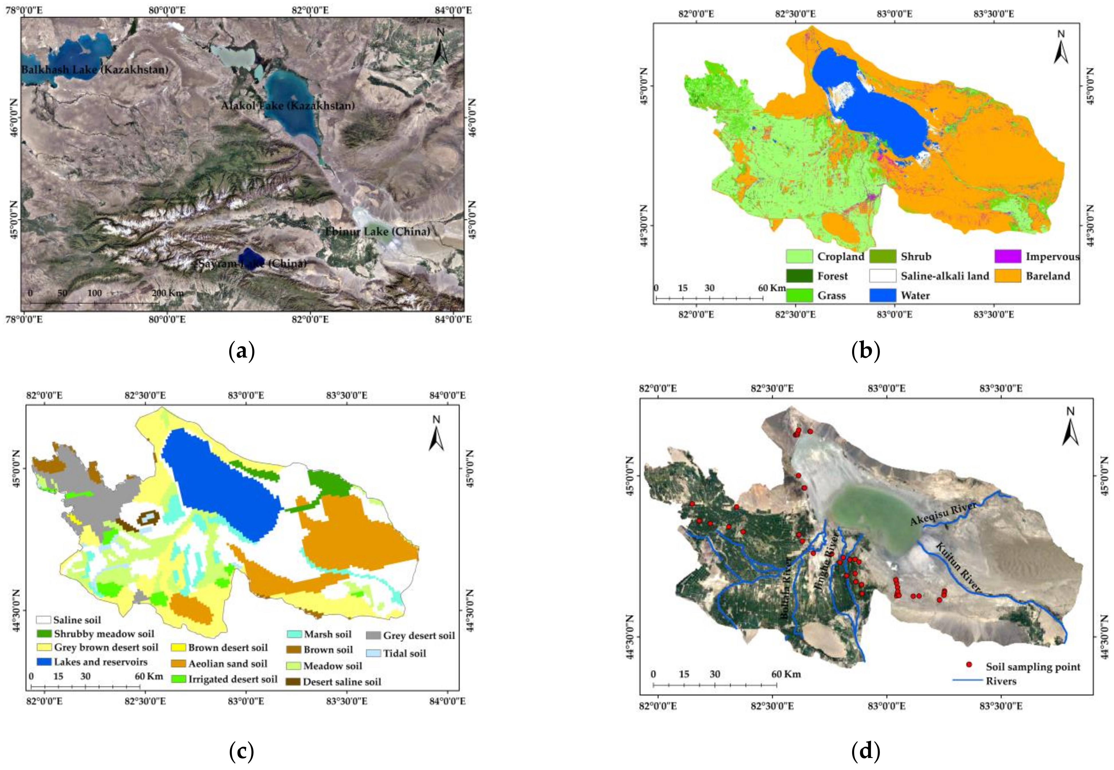
The Ebinur Lake is the largest saltwater lake in Xinjiang, China, situated on the southwest of the Junggar Basin in central Asia [24]. The Ebinur Lake Basin boundary used in this study was obtained from DEM hydrological analysis. The Ebinur Lake Basin is located between 44°24′ N and 45°12′ N, and between 81°56′ E and 83°51′ E (Figure 1a). The Ebinur Lake is at the lowest elevation in the basin, about 189 m. The basin belongs to the temperate continental arid climate, with annual average temperature of 7–8 °C, annual average precipitation of 90.9 mm and evaporation of 1662 mm. The evaporation is much higher than the precipitation. The Boltala River, Jinghe River, Kuitun River and Akeqisu River flow into the lake from different directions, becoming the main water source for the lake area [25], but the incomes are not sufficient, and the lake is shrinking day by day. From 2004 to 2015, the area of the Ebinur Lake in a dry and wet season decreased by 461.98 km2 and 322.04 km2, respectively [26], which greatly accelerated the desertification process in the surrounding areas of the basin. The speed of desertification has reached 38 square kilometers per year. The northwest part of the study area is the Alashan Pass, with 164 days of annual heavy windy days, up to 185 days at most and 55.0 m/s of maximum wind speed [27]. The Ebinur Lake has a high mineralization degree and a prosperous salt ion content. The shrinkage of the lake surface results in the exposure of a large range of dry lake bottom, a large amount of salt dust in the saltwater lake was dried up and exposed to the ground, which causes serious soil salinization. The unique topography of the Ebinur Lake Basin includes a variety of landscapes, such as rocky desert, gravel desert, desert, salt desert, swamp and salty lake. The corresponding typical zonal soil is grey desert soil, grey brown desert soil and aeolian sandy soil, and the intrazonal soil is salt (salinity) soil, meadow soil and marsh soil [28] (Figure 1c). Built on keen wind and abundant salt sources, sandstorms are very common in this area, and salt dust storms frequently erupt [21]. The Ebinur Lake Basin has been the second largest source of salt and dust storms as well as sandstorms in the world. The drought is intensifying, and the ecological environment is deteriorating.
2.2. Field Soil Sampling Experiment
Field soil experiment was made on 15 April 2017. In order to better map the soil moisture and salinity situation in the Ebinur Lake Basin, 60 sampling points were randomly distributed. The distribution of sampling points is shown in Figure 1d. At each sampling point, Stevens Portable Hydra Data Reader (Hydra-Reader) was used to obtain soil basic property data directly with Hydra probe, GPS was used to record longitude and latitude. The probe was cleaned with a polishing cloth before use to avoid increasing the error. In addition, soil specific calibration was required to ensure accuracy before measuring soil moisture [29]. At each sample point, the metal probe of the instrument was inserted vertically clockwise into the soil at a depth of about 5 cm to ensure the full contact of the soil with the metal probe. The response time was 10–20 s. The data posted by the instrument were the actual measured values, including soil type, soil temperature, soil volumetric moisture (m3 m−3), soil electrical conductivity (S/m) and temperature-corrected conductivity (S/m). Hydra-Reader has a data download service for later analysis. The electrical conductivity can be regarded as another form of expression of soil salinity. In this study, soil electrical conductivity was invoked as a measure of soil salinity, and soil volumetric moisture was used as a measure of soil moisture.
In order to ensure the accuracy of the data at the sampling points, we measured each sampling point for 6 times and took the average value as the final value. In addition, a ground object spectrometer was used to measure the reflection spectrum of the sampling point. In order to facilitate the correspondence with Landsat data, we selected the band corresponding to the central wavelength of Landsat band range in the reflection spectrum as the calculation index, so as to reduce the scale problems caused by a direct use of Landsat images. For the measured data of 60 sampling points, we randomly select 35 points as regression fitting data and 25 points as verification analysis data.
2.3. Satellite Image and Data Processing
The Landsat 8 OLI has become the data source of this study because of its convenient acquisition, moderate spatial resolution and rich band information. Its spatial resolution is 30 m, and it is free to access, including 9 bands of information, which are coastal, blue, green, red, near infrared, two short-wave infrared, two thermal infrared, panchromatic (15 m resolution) and cirrus band [30]. The date of image acquisition was 19 April 2017, which was close to the field experiment time, reducing the time error and providing more accurate soil water and salt information. The datum was obtained from the official website of the U.S. Geological Survey (USGS, https://earthexplorer.usgs.gov/ accessed on 30 July 2019).
Landsat 8 OLI data were pre-processed by the ENVI 5.3 software, including radiation calibration, atmospheric correction and mask. The ENVI 5.3 FLAASH module was used for atmospheric correction.
2.3.1. Calculation of Spectral Index
For this study, we selected some spectral indices with a certain universality and applicability related to water and salt, used by previous research institutes, as shown in Table 1. The criterion for index selection is to select those indexes that have been successfully applied in the soil water-salt inversion based on Landsat 8 data, or indexes whose application regions are in arid and semi-arid areas. SI, SI1, SI2, SI3 (four different salinity indices), S1, S2, S3, S4, S5, S6 (six different salinity calculation indicators) and NDSI (normalized salinity index) are salinity indices calculated from remote sensing data, from which surface salinity information can be obtained [31,32]. OLI_SI (Landsat 8 OLI salinity index) is a soil salinity index in an irrigation region based on Landsat 8 data. It has a strong correlation with conductivity EC [33]. SIvir (visible light remote sensing salinity index) is a newly developed spectral salinity index, which has the potential to reveal soil salinity in arid climatic conditions. Int1 and Int2 are intensity indices in the visible light range, BI is a brightness index [34], which can highlight and detect different soil salinity levels [35]. NDWI (normalized water index) and LSWI (land surface water index) are water body indices, which can be used to identify land surface water body and to distinguish moisture in soil. VCI is a vegetation status index, which uses crop growth changes to reflect the degree of water information threatening crops in the region, so that it can express the regional soil moisture difference [36]. VSDI (visible and shortwave infrared drought index) is a surface drought index, which is suitable for different land cover types and less affected by vegetation. It can reflect the difference of surface soil moisture from another perspective [37]. ATI is an apparent thermal inertia, which can reflect the thermal characteristics of soil by the difference of surface temperature. It is closely related to soil moisture and has a useful application in bare soil or low vegetation coverage area [38]. EVI (enhanced vegetation index), NDVI (normalized vegetation index), SAVI (soil-adjusted vegetation index) and OSAVI (optimized soil-adjusted vegetation index) are widely used vegetation indices, which can reflect the growth status of vegetation and soil characteristics.
D1 and D2 are the spectral indices newly created for the soil salinity inversion in arid regions based on the Landsat 8 spectral characteristics of the arid region. We analyze the correlation between various bands of Landsat 8 data and the measured data, select several bands with high correlation, and combine them together. The difference between D1 and D2 is that the weight coefficients of each band is different. The weight coefficients are two sets of data obtained by analyzing the regional environment of the Ebinur Lake Basin.
The above spectral indices were calculated in the Band Math module of ENVI5.3 software.
2.3.2. Inversion of Surface Temperature
The remote sensing inversion method of land surface temperature adopted in this study was the radiation transfer equation method. Its basic principle is to divide the radiation received by the sensor into three parts: surface, up-going and down-going radiation. If the intensity of atmospheric radiation is estimated, the surface radiation intensity can be obtained, and using it, the surface temperature can be calculated. The calculation formula is the Equations (1)–(3) [41].
where L is surface specific emissivity; Ts is surface temperature, the unit is K; B(Ts) is blackbody thermal radiation brightness, Lup and Ldown are upward and downward atmospheric radiations, respectively; is atmospheric transmittance in the thermal infrared band. For Landsat 8 TIRS, K1 = 774.89 w/(m2 × μm × sr), K2 = 1321.08 × K1; τ, ϵ are available on the NASA website (http://atmcorr.gsfc.nasa.gov/ accessed on 30 July 2019).
2.3.3. Construction of Temperature Vegetation Drought Index (TVDI)
TVDI is based on the simplified NDVI-Ts feature space, which is a parameter to represent soil surface characteristics. They consider that there is a certain soil moisture isoline in the characterized space [44]. In NDVI-Ts space, the pixel drought index is 1 on the dry edge, representing complete water shortage; 0 on the wet edge, representing complete water stress; and 0–1 on the data points between the dry and wet edges. The greater the TVDI value, the more serious the relative drought. The TVDI calculation is presented in Equation (4).
where Ts is the surface temperature of a pixel; Tsmin is the lowest temperature (wet edge temperature) at the NDVI value of the pixel; and Tsmax is the highest temperature (dry edge temperature) at the NDVI value of the pixel.
By calculating the maximum and minimum surface temperature corresponding to each NDVI range at a certain interval, the equation of dry edge and wet edge can be fitted (Equations (5) and (6)).
2.3.4. Spike Cap Transformation
Spike cap transform is an orthogonal transformation of a remote sensing image, projecting image information into multi-dimensional space to obtain six components that are important to vegetation, soil and water body, such as greenness, humidity and brightness, and their shapes are similar in multidimensional space. Its shape in multi-dimensional space is the same as that of a hat, so it is called spike cap transformation. Spike cap transformation has been applied to observe the relationship between soil moisture, vegetation cover and canopy conditions [45]. Humidity band can be used to extract soil moisture information. For Landsat 8 OLI images, the conversion coefficient of humidity component is shown in Equation (7).
where B2, B3, B4, B5, B6 and B7 are Landsat 8 blue band (Blue), green band (Green), red band (Red), near infrared band (NIR), short wave infrared 1 (SWIR1) and shortwave infrared 2 (SWIR2), respectively.
2.4. BP Neural Network Model
BP neural network is a multilayer feedforward neural network. Its main characteristics are forward signal transmission and back error propagation. In forward transmission, the input signal is processed layer by layer from the input layer to the output layer. The state of neurons in each layer only affects the state of neurons in the next layer [46]. If the output layer cannot get the expected output, it will turn to back propagation, adjust the weights and thresholds of the network according to the prediction error, so that the predictive output of BP neural network keeps approaching the expected output [47]. Before BP neural network prediction, the network must be trained to have associative memory and prediction ability. The main steps are as follows: (1) network initialization; (2) hidden layer output calculation; (3) output layer output calculation; (4) error calculation; (5) threshold updating. The commonly used algorithm of BP neural network model is gradient descent, which adjusts the changes of threshold and weight of neurons along the direction of negative gradient [48].
It can be seen from the above process that the BP neural network model has strong nonlinear mapping ability and can establish a multivariate nonlinear relationship between independent variables and dependent variables, so it is widely used in remote sensing monitoring. Soil water content is a complex nonlinear coupling system, which is influenced by topography, artificial irrigation and natural environment. Only by fully considering the influence of various factors can the inversion accuracy of soil water content and salt content be improved.
Depending on the characteristics of fitting non-linear function, the BP neural network constructed in this study determined an input parameter, namely various spectral indices, an output parameter, namely soil volume moisture or temperature-corrected conductivity. The BP neural network structure was 1–3–1; that is, there were one node in the input layer, three nodes in the hidden layer and one node in the output layer. All operations were conducted in MATLAB R2015.
2.5. SVR Support Vector Machine Regress Model
Support vector machine (SVM), such as multilayer perceptron network and radial basis function network, can be employed to pattern classification and nonlinear regression [49]. The core idea of an SVM is to establish a classification hyperplane as a decision surface to maximize the isolation edge between positive and negative examples. The theoretical basis of SVR is statistical learning theory, and more precisely, SVR is an approximate realization of structural risk minimization. SVR follows the principle of structural risk minimization and shows advantage in solving small sample, non-linear and high-dimensional pattern recognition problems. Unlike traditional machine learning methods, such as artificial neural networks, which follow the principle of empirical risk minimization, SVR avoids over-fitting, poor local optimization ability, difficulty in parameter adjustment and slow convergence. In support vector machine regression, penalty parameter C and nuclear parameter γ determine the complexity, accuracy and type of the regression model.
The introduction of kernel function can greatly improve the ability of support vector machines to deal with nonlinear problems, and at the same time maintain the intrinsic linearity of support vector machines in high dimensional space. The commonly used kernel functions mainly include linear kernel function, polynomial kernel function, radial basis kernel function and sigmoid kernel function. Since different kernel function types and parameters in SVR have a great influence on the generalization ability of the model, it is necessary to study and determine the kernel function types and parameters. Gaussian radial basis kernel function (RBF kernel function) has a good generalization ability and can support nonlinear regression [50]. In this study, we selected the RBF kernel function.
The grid method is to try the combination of various penalty parameters and RBF kernel function parameters in a certain range, and then conduct data training for each parameter combination and select the parameter combination with the best effect as the optimal parameter [51]. During data training, the k-fold cross-validation method was adopted. N-1 data were set as training data, and the rest were set as test data. The generalization error was determined by the mean value of MSE (root mean square error) after K times of calculation. The grid method parameter optimization is a violent enumeration method; if the amount of data is very large, it is a time-consuming approach, but it is also a very safe approach.
The specific operation was implemented by running the LIBSVM toolkit in the environment of MATLAB R2015b.
2.6. Correlation Analysis Model
Correlation analysis is a statistical analysis method that studies the correlation between two or more random variables with equal statuses. It is a process of describing the closeness of the relationship between objective things and using appropriate statistical indicators. The degree of correlation between the two variables is represented by the correlation coefficient r. The value of the correlation coefficient r is between −1 and 1; it can be any value within this range. In the case of positive correlation, the r value is between 0 and 1, and the scatter plot is obliquely upward. In this case, one variable increases, and the other variable increases. When the correlation is negative, the r value is between −1 and 0, and the scatter plot is diagonally downward, at which point one variable increases and the other variable decreases. The closer the absolute value of r is to 1, the stronger the correlation between the two variables, and the closer the absolute value of r is to 0, the weaker the degree of association between the two variables.
2.7. Statistical Analysis Method
The field observation data were randomly divided into analysis data and verification data, their ratio being 2:1. The basic statistical analysis of the analysis data included correlation analysis, regression analysis, linear and non-linear model fitting accuracy analysis. Among them, Pearson correlation coefficient was used as the correlation index, and its significance test was conducted. Regression analysis refers to a statistical analysis method that determines the quantitative relationship between two or more variables. Regression analysis was performed using analytical data to establish a regression model. The model with superior fitting accuracy was validated and analyzed with validation data, and the index used was root-mean-square error.
3. Results
3.1. Quantitative Analysis Results of Soil Electrical Conductivity and Remote Sensing Index
3.1.1. Correlation between Soil Electrical Conductivity and Remote Sensing Index
The correlation between remote sensing index and soil conductivity is given in Table 2. From Table 2, it can be deduced that: (1) The correlation between B1, B2, B3, B4 in Landsat 8 satellite data and soil salinity was greater than 0.4, so we chose these three bands to build the new salinity indices D1 and D2. (2) The salinity index D2 established for this study had the highest correlation with soil conductivity, followed by OLI_SI. The indexes with correlation coefficients greater than 0.6 were also D1 and Landsat 8 band 1, and their significance was less than 0.001. (3) In Landsat 8 OLI bands, bands 1 and 2 had the highest correlation with soil conductivity, followed by bands 3, 6 and 7, which had almost no correlation. (4) The correlation between vegetation index and soil conductivity was less than 0.4, and the correlation was poor. (5) The correlation between intensity indexes Int1, Int2 and soil conductivity was 0.467 and 0.414, respectively, with good significance, but the correlation of brightness index was poor. (6) The correlation between salinity index and soil conductivity was uneven. The correlation between OLI_SI, S4, S5, D1, D2 and soil conductivity was higher than 0.5, with good significance, while the correlation between S6 was very low and not significant.
3.1.2. Regression Model of Soil Electrical Conductivity
The salinity index D2 was selected as the remote sensing index with the highest correlation and significant correlation with soil electrical conductivity. The regression model with soil conductivity was established. The specific parameters of regression analysis are shown in Table 3, including model formula, fitting accuracy and verification error.
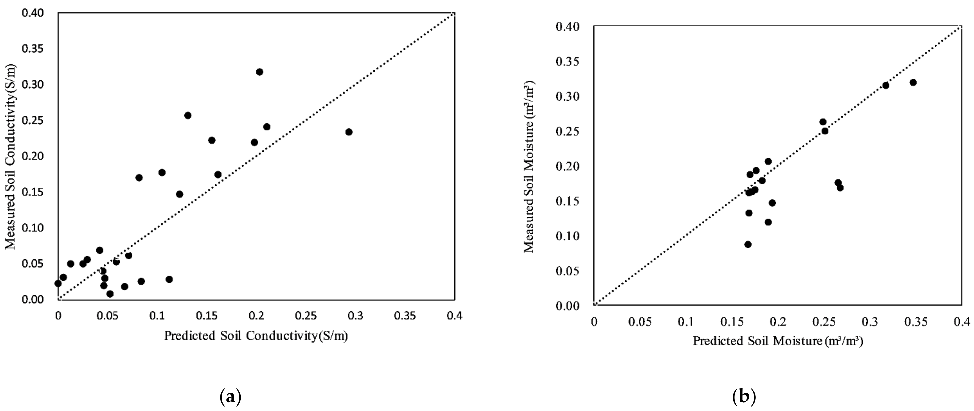
In Table 3, it can be observed that: (1) The regression model of salinity index D2 and soil conductivity had good fitting accuracy. Except for the exponential model, the fitting R2 of other models was greater than 0.5, and the validation error RMSE was less than 0.1 S/m. (2) The BP neural network model had the best fitting accuracy—R2 was 0.624, RMSE was 0.0830 S/m (Figure 2a, verification figure)—followed by cubic function model, where R2 was 0.620, and RMSE was 0.0834 S/m. (3) The fitting accuracy of linear function, quadratic function and SVR model was also greater than 0.6, and RMSE was less than 0.09. (4) In addition, it can be found that although the fitting accuracy of the cubic function model and the quadratic function model was high, the regression coefficients showed the over-fitting phenomenon, and the significance was not high. Therefore, in the final model selection, these two models were excluded. We selected the BP neural network model.
3.2. Quantitative Analysis Results of Soil Volumetric Moisture and Remote Sensing Index
3.2.1. Correlation between Soil Volumetric Moisture and Remote Sensing Index
The correlation between remote sensing index and soil volumetric moisture is presented in Table 4. From Table 4, it can be inferred that: (1) NDWI had the highest and significant correlation with soil volumetric moisture, with R of 0.600, followed by the humidity component of the Spike cap transformation, with R of 0.572. (2) The correlation between Landsat 8 band and soil volumetric moisture was on a general level, B1 and B2 had better correlation, bands 10–11 had almost no correlation, B1–4 had positive correlation, and B5–B7 had negative correlation. (3) Vegetation indices NDVI, EVI, SAVI and VCI negatively correlated with soil volumetric moisture, with good correlations of −0.476, −0.442, −0.498 and −0.476, respectively. (4) LSWI had a low correlation with soil volumetric moisture, while TVDI, VSDI and ATI had poor and insignificant correlation. LST had almost no correlation with surface temperature.
3.2.2. Regression Model of Soil Volumetric Moisture
Among the remote sensing indexes selected by this research institute, NDWI had the highest correlation with soil volumetric moisture. Therefore, the regression model of soil volumetric moisture was established using NDWI. The exact parameters and accuracy of the regression model are shown in Table 5. In Table 5, we can see that: (1) The fitting accuracy of the cubic function model was the best—R2 was 0.538 and RMSE was 0.230—followed by the SVR model and the quadratic function model. (2) The SVR model was not suitable as an inversion model because the fitting R2 was high, but the verification error RMSE was the largest. (3) The fitting accuracy of exponential function was the lowest, and the fitting effect of the primary function was not good. (4) The fitting R2 of the quadratic function was close to that of the cubic function, but the RMSE of the cubic function was smaller (Figure 2b for verification). The significance of the regression parameters was not very different. Therefore, the cubic function was chosen as the remote sensing inversion model of soil volumetric moisture.
3.3. Correlation Analysis of Soil Moisture and Salinity
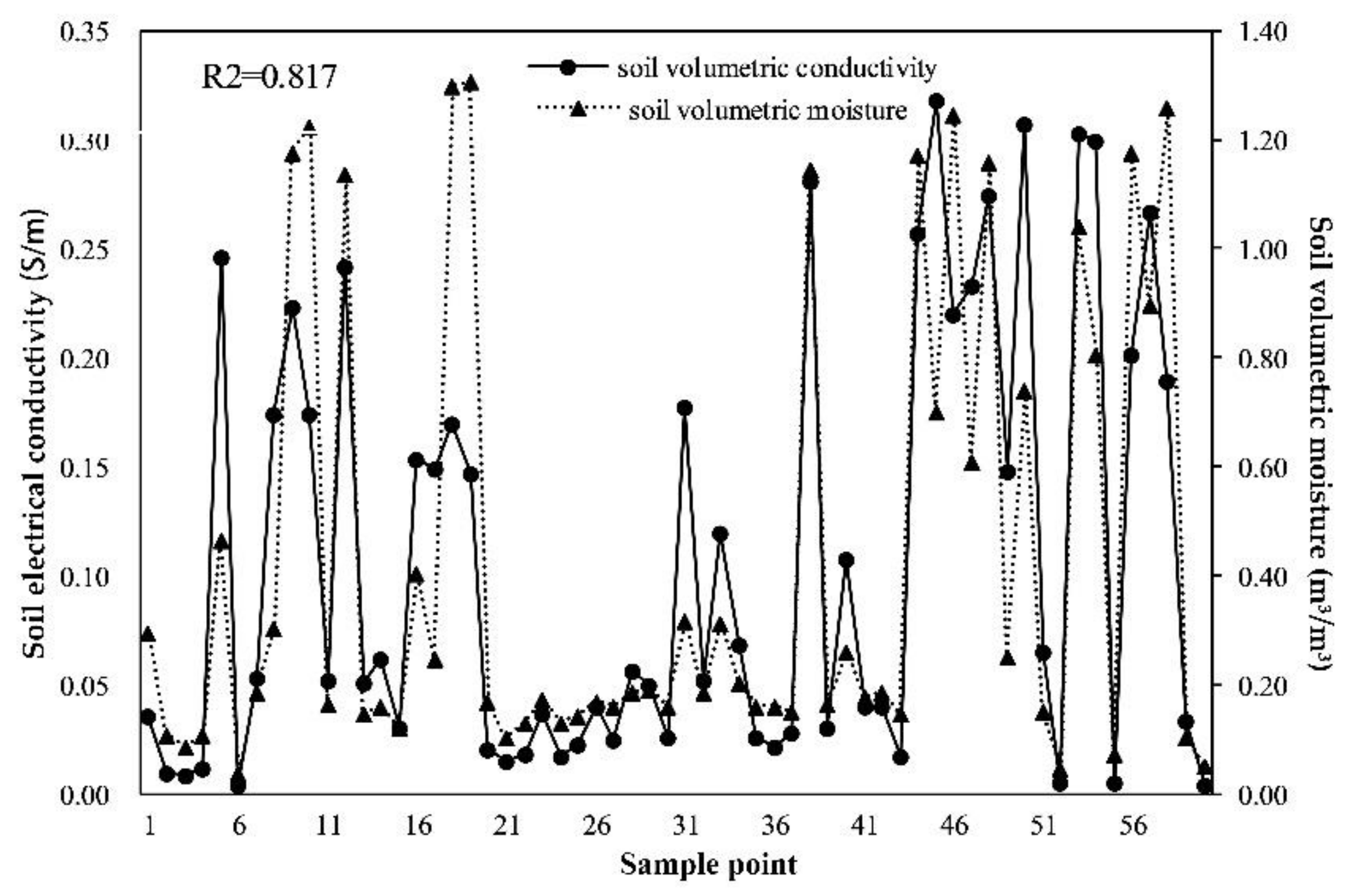
The correlation analysis between soil electrical conductivity and volumetric moisture is shown in Figure 3. From Figure 3, it can be learned that the rules of variation of soil electrical conductivity and soil volumetric moisture tended to be the same, and the correlation degree was 0.817, which meat the synchronous change degree was higher. In other words, the correlation degree between them was higher. In addition, the change rate of soil volumetric moisture at most observation points was higher than that of soil electrical conductivity. The spatial variation rate of soil volumetric moisture was high, and its heterogeneity was strong.
4. Discussion
4.1. Different Rules between Remote Sensing Index and Soil Moisture and Salinity
The correlation between soil electrical conductivity and Landsat 8 bands gradually decreased from B1 to B7, and there was almost no correlation between soil electrical conductivity and B6 and B7. The spectral reflectance of soil electrical conductivity increased with the increase in soil salinity. The 325–600 nm reflectance curve rose sharply with a large amount of information; the 600–1015 nm reflectance curve was flat with no obvious absorption and less information content [52]. Therefore, the correlation of Landsat 8 B1–B4 was significant, and the correlation of the B1 was the greatest. Vegetation index was negatively correlated with soil conductivity; that is, vegetation index was negatively correlated with soil salinity. Vegetation growth is susceptible to soil salinity stress, resulting in impaired photosynthesis and respiration [53]. There are only few salt-tolerant plants in the Ebinur Lake Basin, so the vegetation coverage in the areas with high soil salinity is very low. The purpose of salinity index is to highlight the information of surface salinity, so there is a high correlation between vegetation index with soil conductivity. The correlation between OLI_SI, D1, D2 and soil conductivity was greater than that of other salinity indices. These three indices were proposed for Landsat 8. The expression contained band 1 of Landsat 8, and the correlation between band 1 and soil conductivity was also higher than that of the other bands. Therefore, band 1 should be included in the subsequent study of soil salinity index for Landsat 8.
Soil volumetric moisture was positively correlated with B1–B4 of Landsat 8, and negatively correlated with B5–B7. The reason is that the reflectance spectrum of soil moisture rises rapidly at 300–750 nm with a large amount of information and tends to increase gently at 800–1350 nm with a small amount of information. There are also two steep upward slopes at 1500–1800 nm and 2100–2400 nm [38]. Water index can highlight surface moisture, with a reliable indicator effect on soil moisture. It has a significant positive correlation with soil volume moisture, especially the NDWI and humidity components of the Spike-cap transformation. In theory, the drought index and surface temperature are negatively correlated with soil moisture [12,13], but this study found that drought index and surface temperature were not correlated with soil moisture, so it is not feasible to use drought index to reflect soil moisture laterally. Drought index and surface temperature may affect soil moisture in time resolution. Generally, vegetation index is positively correlated with soil moisture [10], but in this study, vegetation index was negatively correlated with soil volumetric moisture. The reason is that the Ebinur Lake Basin is a high salinity area, where the soil contains too much salt, so that it is difficult for the vegetation to absorb water, and the growth is limited. In addition, the correction analysis of soil water and salt also validated the analysis. The change of soil water and salt was consistent, and soil salinity seriously affected the change of soil water.
4.2. Spatial Distribution of Soil Salt in Ebinur Lake Basin
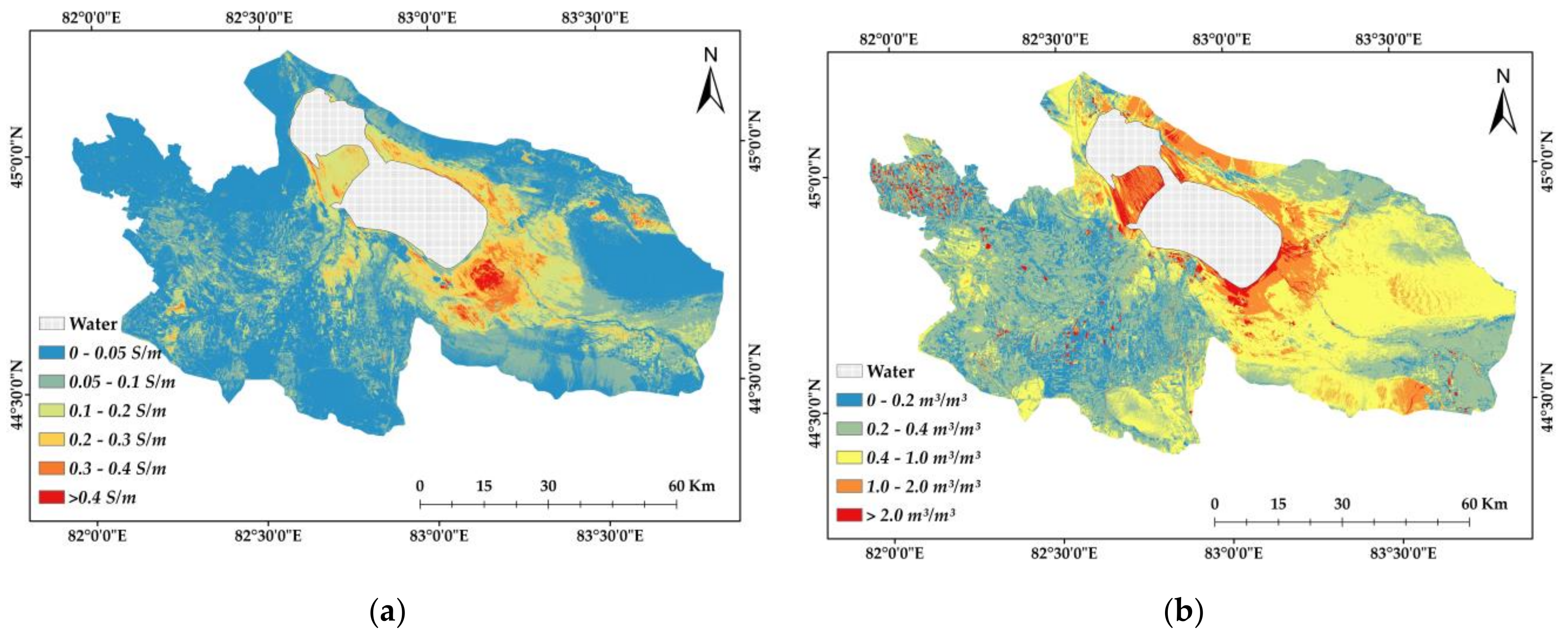
The spatial distribution map of soil salinity in the Ebinur Lake Basin was obtained by model inversion, as shown in Figure 4a. From the figure, it can be seen that the soil salinity in the Ebinur Lake Basin was low around, high in the center, high in the lake area and low in the vegetation coverage area. The soil salinity in the lake area decreased gradually outward. In addition, the salt content along the coast of the Ebinur Lake, Boltala River, Jinghe River, Kuitun River and Akeqisu River is higher than that of other areas. Among them, it was the most obvious in the case of the Ebinur Lake and the Akezisu River. According to the correction analysis of soil water and salt in the Ebinur Lake Basin, the change trend of soil salinity and soil moisture tends to be the same, so in the vicinity of the water area, the soil moisture content is higher than in other areas. There are two distinct white areas in the southeastern part of the Ebinur Lake; namely, the soil electrical conductivity there is greater than 0.4 S/m. These two areas are the Jinghe Salt Field and the Jinghe Old Salt Field respectively, which further confirms the accuracy of the model inversion. The Ebinur Lake is a saltwater lake. The area of the lake is decreasing year by year. The water around the lake is gradually evaporating, and the soil salinity is gradually increasing.
From the above analysis, we can see that the soil salt content is negatively correlated with vegetation coverage. It can be learned that the soil salt content in vegetation coverage area is lower than that in bare land or wetland. In addition, soil salinity of the northern mountain forest is lower than that of the southwestern farmland. In addition to the cause of farmland fertilizer application, the high soil salinity will inhibit the growth of vegetation, so it is also suitable for planting trees and grasslands under the extremely low salinity soil. The area with soil electrical conductivity lower than 0.05 S/m in the eastern part of the country is the Arxi Sea grassland, which further validates the above discussion.
Salinization is part of the main causes of soil degradation in arid and semi-arid regions of the world. It inhibits plant growth and agricultural production and aggravates soil erosion. Nearly 20% of land in China is influenced by salinization, which is increasing with human activities, especially in arid and semi-arid areas [54]. As a typical arid and semi-arid region and an important geographic unit in central Asia, monitoring and mapping of the Ebinur Lake Basin soil salinity over a long period of time and wide space are of great significance for curbing soil degradation and sustainable agricultural production.
4.3. Spatial Distribution of Soil Moisture in Ebinur Lake Basin
The spatial distribution of soil moisture in the Ebinur Lake Basin was retrieved from the cubic regression model, as shown in Figure 4b. As can be seen on the map, soil moisture in the Ebinur Lake Basin gradually decreased outward with the Ebinur Lake as the center and was higher in the west and lower in the east. There were many white spots (i.e., soil volumetric moisture > 2 m3 m−3). In the southwest of the basin, the bright spot was the Panqiao fishpond and in the northwest, paddy fields and reservoirs. This area was the same as the lake, so the soil moisture in this area was very high. Soil volumetric moisture along the coast of the Ebinur Lake, recharged by lake water, was 1–2 m3 m−3. The soil moisture in this kind of area is also higher than that in other areas. Because of poor water storage capacity of inland saline soil, the soil moisture of inland saline soil is lower than that of other regions. The soil moisture along the four rivers is 1–2 m3 m−3, which conforms to the basic natural law.
Soil moisture content of the farmland in the west is low, and the type of soil is inland saline soil, which is not conducive to the growth of crops, but affected by topography, it developed into farmland. Under the influence of water stress, the yield of crops is low. Soil water loss is a major restrictive factor for land degradation in arid and semi-arid areas [55]. Vegetation is very vulnerable to water stress, which has a huge impact on agricultural production [56]. Therefore, timely and accurate dynamic grasp of soil moisture changes in arid and semi-arid areas is of great significance for ecological development.
4.4. Relevant Rules of Soil Water and Salt
According to the correlation analysis of soil water and salt in the Ebinur Lake Basin, the change trend of the two tended to be consistent. Depending on the physical characteristics of soil, soil water is the carrier of soil salt transport. As can be seen in Figure 4, the soil salinity was extremely high and the soil moisture was also large around the Ebinur Lake, and the two changes were related. In the eastern, southern and northwestern parts of the basin, the conductivity of soil volumetric was less than 0.05 S/m, the salinity was very low, but the soil moisture content was high. Soil moisture content was high, which has a definite dilution effect on soil salinity. Soil water and salt are related and interrelated. Especially in arid and semi-arid areas, the change of soil water and salt is one of the controlling factors in the formation of saline land [56]. It is of great significance to study the correlation and linkage effects of soil water and salt for soil restoration and inhibition of land desertification and degradation in arid areas.
4.5. Data Accuracy Discussion
The field experiment for this study was carried out in the Ebinur Lake in May, and the measurement were performed for only one year. Although multiple measurements were taken for each measurement point and their average value was taken into consideration, the inversion model of this study is not universal due to the lack of long-term continuous observation data. In arid areas, soil moisture and salt content change with the year and season. As a result, the spectral characteristics of the ground surface will change, the inversion index will also change, and the final inversion model and results will also be different. Therefore, the important direction for the future research is to study the influence of different measurement periods on the selection of soil water content and salinity inversion index, and to explore whether there is an inversion model that is more universal for all time periods.
5. Conclusions
In this study, based on a series of field experiment data of soil salinity, soil moisture and remote sensing data (from Landsat 8 OLI), the remote sensing index for estimating soil water and salt content in the Ebinur Lake Basin were tested and compared, and two new salinity indices for Landsat 8 were developed. Good models for inversion of soil moisture and salinity in the Ebinur Lake Basin were tested and obtained. The spatial distribution of soil water and salt in the Ebinur Lake Basin was predicted using the remote sensing data. The research results of this paper have certain guiding significance for the future geophysical process modeling of water and salt transport in arid saline lake basins. The basic conclusions of this study are as follows:
- (1)
- Among the various indexes for estimating soil salinity in the Ebinur Lake Basin, the salinity index had a greater advantage than the vegetation index, and the correlation between the newly established salinity index D2 and soil conductivity was as high as 0.650. The accuracy of the BP neural network salt prediction model based on this index was also higher than other models (R2 = 0.624, RMSE = 0.083).
- (2)
- For the soil moisture content in the Ebinur Lake Basin, the correlation of the normalized water index (NDWI) was greater than that of other indices (R = 0.600). The cubic function prediction model had the best effect, the fitting accuracy was 0.538, and the verification error was 0.230.
- (3)
- The correlation degree of soil water and salinity was very high, reaching 0.817. The two trends tended to be the same, but the spatial mutation rate of soil moisture was high and heterogeneity was strong.
- (4)
- The soil salinity in the Ebinur Lake Basin was low around, high in the center, high in the lake area and low in the vegetation coverage area, and the soil salinity in the lake area decreased gradually outward. The soil moisture in the Ebinur Lake Basin gradually decreased outward with the Ebinur Lake as the center and was higher in the west and lower in the east, with more small ponds.
Author Contributions
This paper was written by J.W., D.L. reviewed and improved the manuscript with comments; the data compilation and statistical analyses were completed by J.W., W.W., Y.H., S.T., D.L. All authors have read and agreed to the published version of the manuscript.
Funding
This project is supported by Inner Mongolia major science and technology project (ZDZX2018054).
Institutional Review Board Statement
Not applicable.
Informed Consent Statement
Not applicable.
Data Availability Statement
Not applicable.
Conflicts of Interest
The authors declare no conflict of interest.
References
- Gkiougkis, I.; Kallioras, A.; Pliakas, F.; Pechtelidis, A.; Diamantis, V.; Diamantis, I.; Ziogas, A.; Dafnis, I. Assessment of soil salinization at the eastern Nestos River Delta, N.E. Greece. Catena 2015, 128, 238–251. [Google Scholar] [CrossRef]
- Sadeghravesh, M.H.; Khosravi, H.; Ghasemian, S. Assessment of combating-desertification strategies using the linear assignment method. Solid Earth 2016, 7, 673–683. [Google Scholar] [CrossRef] [Green Version]
- Hamzeh, S.; Naseri, A.A.; AlaviPanah, S.K.; Mojaradi, B.; Bartholomeus, H.M.; Clevers, J.G.P.W.; Behzad, M. Estimating salinity stress in sugarcane fields with spaceborne hyperspectral vegetation indices. Int. J. Appl. Earth Obs. Geoinf. 2013, 21, 282–290. [Google Scholar] [CrossRef]
- Periasamy, S.; Shanmugam, R.S. Multispectral and Microwave Remote Sensing Models to Survey Soil Moisture and Salinity. Land Degrad. Dev. 2017, 28, 1412–1425. [Google Scholar] [CrossRef]
- Odunze, A.C.; Mando, A.; Sogbedji, J.; Amapu, I.Y.; Tarfa, B.D.; Yusuf, A.A.; Sunday, A.; Bello, H. Moisture conservation and fertilizer use for sustainable cotton production in the sub-humid Savanna zones of Nigeria. Arch. Agron. Soil Sci. 2012, 58, S190–S194. [Google Scholar] [CrossRef]
- Han, L.; Liu, D.; Cheng, G.; Zhang, G.; Wang, L. Spatial distribution and genesis of salt on the saline playa at Qehan Lake, Inner Mongolia, China. Catena 2019, 177, 22–30. [Google Scholar] [CrossRef]
- Wagner, W.; Naeimi, V.; Scipal, K.; de Jeu, R.; Martínez-Fernández, J. Soil moisture from operational meteorological satellites. Hydrogeol. J. 2006, 15, 121–131. [Google Scholar] [CrossRef]
- Mallick, J.; AlMesfer, M.K.; Singh, V.P.; Falqi, I.I.; Singh, C.K.; Alsubih, M.; Kahla, N.B. Evaluating the NDVI–Rainfall Relationship in Bisha Watershed, Saudi Arabia Using Non-Stationary Modeling Technique. Atmosphere 2021, 12, 593. [Google Scholar] [CrossRef]
- Kumari, N.; Srivastava, A.; Dumka, U.C. A Long-Term Spatiotemporal Analysis of Vegetation Greenness over the Himalayan Region Using Google Earth Engine. Climate 2021, 9, 109. [Google Scholar] [CrossRef]
- Fakharizadehshirazi, E.; Sabziparvar, A.A.; Sodoudi, S. Long-term spatiotemporal variations in satellite-based soil moisture and vegetation indices over Iran. Environ. Earth Sci. 2019, 78, 342. [Google Scholar] [CrossRef]
- Hosseini, M.; Saradjian, M.R. Multi-index-based soil moisture estimation using MODIS images. Int. J. Remote Sens. 2011, 32, 6799–6809. [Google Scholar] [CrossRef]
- Zhu, W.; Jia, S.; Lv, A. A time domain solution of the Modified Temperature Vegetation Dryness Index (MTVDI) for continuous soil moisture monitoring. Remote Sens. Environ. 2017, 200, 1–17. [Google Scholar] [CrossRef]
- Liu, Z.; Zhao, Y. Research on the method for retrieving soil moisture using thermal inertia model. Sci. China Ser. D 2006, 49, 539–545. [Google Scholar] [CrossRef]
- Sinha, A. Variations in soil spectral reflectance related to soil moisture, organic matter and particle size. J. Indian Soc. Remote Sens. 1987, 15, 7–11. [Google Scholar] [CrossRef]
- Yanjun, S.; Ying, G.; Zhaoyan, J. Monitoring soil moisture by apparent thermal intertia method. Chin. J. Eco Agric. 2011, 19, 1157–1161. [Google Scholar]
- Ghulam, A.; Qin, Q.; Teyip, T.; Li, Z.L. Modified perpendicular drought index (MPDI): A real-time drought monitoring method. ISPRS J. Photogramm. Remote Sens. 2007, 62, 150–164. [Google Scholar] [CrossRef]
- Zhang, J.; Zhang, Q.; Bao, A.; Wang, Y. A New Remote Sensing Dryness Index Based on the Near-Infrared and Red Spectral Space. Remote Sens. 2019, 11, 456. [Google Scholar] [CrossRef] [Green Version]
- Gorrab, A.; Zribi, M.; Baghdadi, N.; Lili-Chabaane, Z.; Mougenot, B. Multi-frequency analysis of soil moisture vertical heterogeneity effect on radar backscatter. In Proceedings of the 2014 1st International Conference on Advanced Technologies for Signal and Image Processing (ATSIP), Sousse, Tunisia, 17–19 March 2014; pp. 379–384. [Google Scholar]
- Choker, M.; Baghdadi, N.; Zribi, M.; El Hajj, M.; Paloscia, S.; Verhoest, N.E.; Lievens, H.; Mattia, F. Evaluation of the Oh, Dubois and IEM models using large dataset of SAR signal and experimental soil measurements. Water 2017, 9, 38. [Google Scholar] [CrossRef]
- Bindlish, R.; Jackson, T.; Gasiewski, A.; Klein, M.; Njoku, E. Soil moisture mapping and AMSR-E validation using the PSR in SMEX02. Remote Sens. Environ. 2006, 102, 127–139. [Google Scholar] [CrossRef]
- Wang, X.; Zhang, F.; Ding, J.; Kung, H.T.; Latif, A.; Johnson, V.C. Estimation of soil salt content (SSC) in the Ebinur Lake Wetland National Nature Reserve (ELWNNR), Northwest China, based on a Bootstrap-BP neural network model and optimal spectral indices. Sci. Total Environ. 2018, 615, 918–930. [Google Scholar] [CrossRef]
- Acar, H.; Ozerdem, M.; Acar, E. Soil Moisture Inversion Via Semiempirical and Machine Learning Methods With Full-Polarization Radarsat-2 and Polarimetric Target Decomposition Data: A Comparative Study. IEEE Access 2020, 8, 197896–197907. [Google Scholar] [CrossRef]
- Bannari, A.; Guedon, A.M.; El-Harti, A.; Cherkaoui, F.Z.; El-Ghmari, A. Characterization of Slightly and Moderately Saline and Sodic Soils in Irrigated Agricultural Land using Simulated Data of Advanced Land Imaging (EO-1) Sensor. Commun. Soil Sci. Plant Anal. 2008, 39, 2795–2811. [Google Scholar] [CrossRef]
- Wang, J.; Ding, J.; Li, G.; Liang, J.; Yu, D.; Aishan, T.; Zhang, F.; Yang, J.; Abulimiti, A.; Liu, J. Dynamic detection of water surface area of Ebinur Lake using multi-source satellite data (Landsat and Sentinel-1A) and its responses to changing environment. Catena 2019, 177, 189–201. [Google Scholar] [CrossRef]
- Mo, K.; Chen, Q.; Chen, C.; Zhang, J.; Wang, L.; Bao, Z. Spatiotemporal variation of correlation between vegetation cover and precipitation in an arid mountain-oasis river basin in northwest China. J. Hydrol. 2019, 574, 138–147. [Google Scholar] [CrossRef]
- Zhu, X. Study on the Dynamic Change of Ebinur Lake Based on Multi-Source Remote Sensing Data. Master’s Thesis, Xinjiang University, Xinjiang, China, 2018. [Google Scholar]
- Zeng, H.; Wu, B.; Zhu, W.; Zhang, N. A trade-off method between environment restoration and human water consumption: A case study in Ebinur Lake. J. Clean. Prod. 2019, 217, 732–741. [Google Scholar] [CrossRef]
- Qian, Y.; Wu, Z.; Zhang, L.; Zhou, H.; Wu, S.; Yang, Q. Eco-environmental evolution, control, and adjustment for Aibi Lake catchment. Environ. Manag. 2005, 36, 506–517. [Google Scholar] [CrossRef]
- Vaz, C.M.P.; Jones, S.; Meding, M.; Tuller, M. Evaluation of Standard Calibration Functions for Eight Electromagnetic Soil Moisture Sensors. Vadose Zone J. 2013, 12, vzj2012.0160. [Google Scholar] [CrossRef]
- Peng, J.; Biswas, A.; Jiang, Q.; Zhao, R.; Hu, J.; Hu, B.; Shi, Z. Estimating soil salinity from remote sensing and terrain data in southern Xinjiang Province, China. Geoderma 2019, 337, 1309–1319. [Google Scholar] [CrossRef]
- Allbed, A.; Kumar, L.; Aldakheel, Y.Y. Assessing soil salinity using soil salinity and vegetation indices derived from IKONOS high-spatial resolution imageries: Applications in a date palm dominated region. Geoderma 2014, 230–231, 1–8. [Google Scholar] [CrossRef]
- Ennaji, W.; Barakat, A.; Karaoui, I.; El Baghdadi, M.; Arioua, A. Remote sensing approach to assess salt-affected soils in the north-east part of Tadla plain, Morocco. Geol. Ecol. Landsc. 2018, 2, 22–28. [Google Scholar] [CrossRef] [Green Version]
- El Harti, A.; Lhissou, R.; Chokmani, K.; Ouzemou, J.-E.; Hassouna, M.; Bachaoui, E.M.; El Ghmari, A. Spatiotemporal monitoring of soil salinization in irrigated Tadla Plain (Morocco) using satellite spectral indices. Int. J. Appl. Earth Obs. Geoinf. 2016, 50, 64–73. [Google Scholar] [CrossRef]
- Bouaziz, M.; Matschullat, J.; Gloaguen, R. Improved remote sensing detection of soil salinity from a semi-arid climate in Northeast Brazil. Comptes Rendus Geosci. 2011, 343, 795–803. [Google Scholar] [CrossRef]
- Triki Fourati, H.; Bouaziz, M.; Benzina, M.; Bouaziz, S. Modeling of soil salinity within a semi-arid region using spectral analysis. Arab. J. Geosci. 2015, 8, 11175–11182. [Google Scholar] [CrossRef]
- Zhang, J.-H.; Zhou, Z.; Yao, F.; Yang, L.; Hao, C. Validating the Modified Perpendicular Drought Index in the North China Region Using In Situ Soil Moisture Measurement. IEEE Geosci. Remote. Sens. Lett. 2015, 12, 542–546. [Google Scholar] [CrossRef]
- Zhang, N.; Hong, Y.; Qin, Q.; Liu, L. VSDI: A visible and shortwave infrared drought index for monitoring soil and vegetation moisture based on optical remote sensing. Int. J. Remote Sens. 2013, 34, 4585–4609. [Google Scholar] [CrossRef]
- Song, C.; Jia, L. A Method for Downscaling FengYun-3B Soil Moisture Based on Apparent Thermal Inertia. Remote Sens. 2016, 8, 703. [Google Scholar] [CrossRef] [Green Version]
- Huete, A.R. A soil-adjusted vegetation index (SAVI). Remote Sens. Environ. 1988, 25, 295–309. [Google Scholar] [CrossRef]
- Douaoui, A.E.K.; Nicolas, H.; Walter, C. Detecting salinity hazards within a semiarid context by means of combining soil and remote-sensing data. Geoderma 2006, 134, 217–230. [Google Scholar] [CrossRef]
- Cao, X.; Cui, X.; Yue, M.; Chen, J.; Tanikawa, H.; Ye, Y. Evaluation of wildfire propagation susceptibility in grasslands using burned areas and multivariate logistic regression. Int. J. Remote Sens. 2013, 34, 6679–6700. [Google Scholar] [CrossRef]
- Zhang, Y.; Song, C.; Sun, G.; Band, L.E.; Noormets, A.; Zhang, Q. Understanding moisture stress on light use efficiency across terrestrial ecosystems based on global flux and remote-sensing data. J. Geophys. Res. Biogeosci. 2015, 120, 2053–2066. [Google Scholar] [CrossRef]
- Sandholt, I.; Rasmussen, K.; Andersen, J. A simple interpretation of the surface temperature/vegetation index space for assessment of surface moisture status. Remote Sens. Environ. 2002, 79, 213–224. [Google Scholar] [CrossRef]
- Mostafiz, C.; Chang, N.-B. Tasseled cap transformation for assessing hurricane landfall impact on a coastal watershed. Int. J. Appl. Earth Obs. Geoinf. 2018, 73, 736–745. [Google Scholar] [CrossRef]
- Lyu, X.; Li, X.; Gong, J.; Li, S.; Huashun, D.; Dang, D.; Xuan, X.; Wang, H. Remote-sensing inversion method for aboveground biomass of typical steppe in Inner Mongolia, China. Ecol. Indic. 2020, 120, 106883. [Google Scholar] [CrossRef]
- Hassan-Esfahani, L.; Torres-Rua, A.; Jensen, A.; McKee, M. Assessment of Surface Soil Moisture Using High-Resolution Multi-Spectral Imagery and Artificial Neural Networks. Remote Sens. 2015, 7, 2627–2646. [Google Scholar] [CrossRef] [Green Version]
- Song, Q.; Wu, Y.; Soh, Y.C. Robust Adaptive Gradient-Descent Training Algorithm for Recurrent Neural Networks in Discrete Time Domain. IEEE Trans. Neural Netw. 2008, 19, 1841–1853. [Google Scholar] [CrossRef]
- Jiang, H.; Rusuli, Y.; Amuti, T.; He, Q. Quantitative assessment of soil salinity using multi-source remote sensing data based on the support vector machine and artificial neural network. Int. J. Remote Sens. 2018, 40, 284–306. [Google Scholar] [CrossRef]
- Hong, X.; Chen, S.; Qatawneh, A.; Daqrouq, K.; Sheikh, M.; Morfeq, A. Sparse probability density function estimation using the minimum integrated square error. Neurocomputing 2013, 115, 122–129. [Google Scholar] [CrossRef]
- Wang, X.L.; Li, Z.B. Identifying the parameters of the kernel function in support vector machines based on the grid-search method. Period. Ocean Univ. China 2005, 35, 859–862. [Google Scholar]
- Zhang, F. Study on the Spectral Characteristics of Salinized Soils with Ground Objects in the Typical Oasis of Arid Area; Xinjiang University: Xinjinag, China, 2011. [Google Scholar]
- Fatma, M.; Asgher, M.; Masood, A.; Khan, N.A. Excess sulfur supplementation improves photosynthesis and growth in mustard under salt stress through increased production of glutathione. Environ. Exp. Bot. 2014, 107, 55–63. [Google Scholar] [CrossRef]
- Li, J.; Pu, L.; Han, M.; Zhu, M.; Zhang, R.; Xiang, Y. Soil salinization research in China: Advances and prospects. J. Geogr. Sci. 2014, 24, 943–960. [Google Scholar] [CrossRef]
- Ostovari, Y.; Ghorbani-Dashtaki, S.; Bahrami, H.-A.; Naderi, M.; Dematte, J.A.M. Soil loss estimation using RUSLE model, GIS and remote sensing techniques: A case study from the Dembecha Watershed, Northwestern Ethiopia. Geoderma Reg. 2017, 11, 28–36. [Google Scholar] [CrossRef]
- Zhou, Q.; Luo, Y.; Zhou, X.; Cai, M.; Zhao, C. Response of vegetation to water balance conditions at different time scales across the karst area of southwestern China-A remote sensing approach. Sci. Total Environ. 2018, 645, 460–470. [Google Scholar] [CrossRef] [PubMed]
- Sun, H. Dynamic Water and Salt Changes in Saline Wasteland on the Lower Edge of Plain Reservoirs in the Desert Oasis Region. Asian Agric. Res. 2018, 10, 23–33. [Google Scholar]
Figure 1.
General map of the study area: (a) location of the study area; (b) land use in the Ebinur Lake Basin; (c) soil type in the Ebinur Lake Basin; (d) distribution map of soil sampling points.
Figure 1.
General map of the study area: (a) location of the study area; (b) land use in the Ebinur Lake Basin; (c) soil type in the Ebinur Lake Basin; (d) distribution map of soil sampling points.

Figure 2.
(a) Comparison of measured and predicted soil conductivity; (b) comparison of measured and predicted soil moisture.
Figure 2.
(a) Comparison of measured and predicted soil conductivity; (b) comparison of measured and predicted soil moisture.

Figure 3.
Simultaneous change of soil electrical conductivity and volume of soil water.

Figure 4.
(a) Spatial distribution of soil electrical conductivity (S/m); (b) spatial distribution of soil volumetric moisture (m3 m−3).
Figure 4.
(a) Spatial distribution of soil electrical conductivity (S/m); (b) spatial distribution of soil volumetric moisture (m3 m−3).

Table 1.
Spectral indices and their calculation formulas.
| Index | Formula | Reference | Index | Formula | Reference |
|---|---|---|---|---|---|
| BI | [31] | S6 | [31] | ||
| EVI | [34] | SI | [32] | ||
| SAVI | [39] | SI1 | [40] | ||
| Int1 | [34] | SI2 | [40] | ||
| Int2 | [34] | SI3 | [40] | ||
| OLI_SI | [33] | NDWI | [11] | ||
| OSAVI | [41] | LSWI | [42] | ||
| S1 | [31] | VCI | [43] | ||
| S2 | [31] | VSDI | [37] | ||
| S3 | [31] | ATI | [38] | ||
| S4 | [31] | SIvir | [35] | ||
| S5 | [31] | ||||
| D1 | |||||
| D2 | |||||
Note: RCoastal, RGreen, RBlue, RRed, RNIR, RSWIR are the corresponding bands of Landsat 8, NDVImin is NDVI minimum, NDVImax is NDVI maximum, the pixel-by-pixel value is NDVIi, α is full-band reflectance; Td, Tn are daytime and night temperatures on the same day, respectively.
Table 2.
Correlation coefficients between soil electrical conductivity and remote sensing indexes.
| Index | R | Index | R | Index | R |
|---|---|---|---|---|---|
| B1 | 0.612 ** | OSAVI | −0.358 ** | S5 | 0.521 ** |
| B2 | 0.589 ** | Int1 | 0.467 ** | S6 | 0.127 |
| B3 | 0.507 ** | Int2 | 0.414 ** | SI | 0.495 ** |
| B4 | 0.425 ** | BI | 0.349 ** | SI1 | 0.469 ** |
| B5 | 0.257 * | NDSI | 0.361 ** | SI2 | 0.404 ** |
| B6 | 0.046 | OLI_SI | 0.637 ** | SI3 | 0.465 ** |
| B7 | −0.066 | S1 | 0.303 * | SIvir | 0.341 ** |
| EVI | −0.274 * | S2 | 0.312 * | D1 | 0.630 ** |
| SAVI | −0.359 ** | S3 | 0.330 ** | D2 | 0.650 ** |
| NDVI | −0.361 ** | S4 | 0.515 ** | ASI | 0.391 ** |
Note: B1, B2, B3, B4, B5, B6 and B7 are Landsat 8 coastal band, blue band, green band, red band, near infrared band, short wave infrared 1 and shortwave infrared 2, respectively; * p < 0.05; ** p < 0.01.
Table 3.
Regression model and accuracy of remote sensing index and soil conductivity.
| Variable | Formula | Sig | R2 | RMSE |
|---|---|---|---|---|
| D2 | Sig1 = 0.003, Sig2 = 0.818 | 0.497 | 0.1213 | |
| Sig1 = 0.000, Sig2 = 0.035 | 0.607 | 0.0855 | ||
| Sig1 = 0.000, Sig2 = 0.000 | 0.573 | 0.0936 | ||
| Sig1 = 0.261, Sig2 = 0.048 Sig3 = 0.260 | 0.609 | 0.0862 | ||
| Sig1 = 0.074, Sig2 = 0.074 Sig3 = 0.074, Sig4 = 0.062 | 0.620 | 0.0834 | ||
| Sig1 = 0.001, Sig2 = 0.092 | 0.503 | 0.0928 | ||
| BP | Sig = 0.000 | 0.624 | 0.0830 | |
| SVR | Sig = 0.001 | 0.497 | 0.1213 |
Note: Sig is the significance of the regression coefficient. If its value is 0.01 < Sig < 0.05, the difference is significant, and if Sig < 0.01, the difference is extremely significant. Sig1, Sig2, Sig3, Sig4 are the significances of the first, second, third and fourth coefficient, respectively.
Table 4.
Coefficient of correlation between soil volumetric moisture and remote sensing indexes.
| Index | R | Index | R |
|---|---|---|---|
| B1 | 0.468 ** | EVI | −0.442 ** |
| B2 | 0.435 ** | SAVI | −0.498 ** |
| B3 | 0.330 ** | NDWI | 0.600 ** |
| B4 | 0.209 | LSWI | 0.358 ** |
| B5 | −0.063 | TVDI | −0.118 |
| B6 | −0.288 * | VCI | −0.476 ** |
| B7 | −0.350 ** | VSDI | 0.231 |
| B10 | −0.011 | ATI | 0.171 |
| B11 | 0.027 | Wetness | 0.572 ** |
| NDVI | −0.476 ** | LST | −0.006 |
Note: * p < 0.05, ** p < 0.01.
Table 5.
Regression model and accuracy of remote sensing index and soil volumetric moisture.
| Variable | Formula | Sig | R2 | RMSE |
|---|---|---|---|---|
| NDWI | Sig1 = 0.028, Sig2 = 0.000 | 0.323 | 0.277 | |
| Sig1 = 0.001, Sig2 = 0.000 | 0.418 | 0.331 | ||
| Sig1 = 0.000, Sig2 = 0.000 Sig3 = 0.000 | 0.531 | 0.275 | ||
| Sig1 = 0.000, Sig2 = 0.003 Sig3 = 0.021, Sig4 = 0.000 | 0.538 | 0.230 | ||
| BP | Sig = 0.001 | 0.502 | 0.277 | |
| SVR | Sig = 0.003 | 0.534 | 0.389 |
Publisher’s Note: MDPI stays neutral with regard to jurisdictional claims in published maps and institutional affiliations. |
© 2021 by the authors. Licensee MDPI, Basel, Switzerland. This article is an open access article distributed under the terms and conditions of the Creative Commons Attribution (CC BY) license (https://creativecommons.org/licenses/by/4.0/).
Share and Cite
MDPI and ACS Style
Wang, J.; Wang, W.; Hu, Y.; Tian, S.; Liu, D. Soil Moisture and Salinity Inversion Based on New Remote Sensing Index and Neural Network at a Salina-Alkaline Wetland. Water 2021, 13, 2762. https://doi.org/10.3390/w13192762
AMA Style
Wang J, Wang W, Hu Y, Tian S, Liu D. Soil Moisture and Salinity Inversion Based on New Remote Sensing Index and Neural Network at a Salina-Alkaline Wetland. Water. 2021; 13(19):2762. https://doi.org/10.3390/w13192762
Chicago/Turabian StyleWang, Jie, Weikun Wang, Yuehong Hu, Songni Tian, and Dongwei Liu. 2021. "Soil Moisture and Salinity Inversion Based on New Remote Sensing Index and Neural Network at a Salina-Alkaline Wetland" Water 13, no. 19: 2762. https://doi.org/10.3390/w13192762
Note that from the first issue of 2016, this journal uses article numbers instead of page numbers. See further details here.