Abstract
Flooding has presented a significant risk for urban areas around the world. Road inundation is one of the severe consequences leading to traffic issues and congestion. Green infrastructure (GI) offers further potential for stormwater management as an environmentally friendly and sustainable solution. However, sewer system behaviour has been overlooked in GI implementation. This study investigates sewer performance by measuring topological connectivity and hydraulic characteristics, and critical components are identified under different design storms. Three retrofit scenarios, including enlarged pipes (grey infrastructure, Grey I), rain gardens (GI), and the combination of enlarged pipes and increased rain gardens (GI + Grey I), are proposed according to the distribution of critical components. The results show that it is feasible to locate the vulnerable parts of the sewer system and GI site allocations based on the critical components that significantly impact the performance of the entire system. While all three scenarios can mitigate inundation, GI and GI + Grey I perform better than pipe enlargement, especially for runoff reduction during long-duration rainfall. Furthermore, the sewer behaviour and retrofit effect are dynamic under different rainfall patterns, leading to diverse combined effects. The discoveries reveal that the adaptation measures should combine with sewer behaviour and local rainfall characteristics to enhance stormwater management.
1. Introduction
Flood risk has been increasing as urbanisation and climate change continue to intensify [1,2,3,4]. The insufficient capacity of drainage systems in over-exploited urban areas has increased road inundation frequency [5,6,7,8]. Although the drainage system has been improved continuously as legacy infrastructure, the uncertainty of environmental change (e.g., urban development or precipitation patterns shifting) and facility ageing inevitably increase burden and vulnerability on the drainage system [9]. As a result, numerous strategies and technologies have been proposed to strengthen urban resilience and infrastructure sustainability against inundation [10,11,12,1313]. The conventional control method, also termed grey infrastructure (Grey I), emphasises structural measures such as adding interception pipes, expanding detention inside sewer pipes, or building end-of-pipe stormwater tanks. The structural stability and lower sensitivity to external disturbances make grey infrastructure indispensable in flood reduction. However, this has been proven to be unfriendly to the environment, and the additional space and maintenance required are costly [14]. Chen et al. [15] investigated the effect of grey infrastructure on flood reduction and concluded that even a large civil engineering scheme such as a deep tunnel system has limited mitigation for inundation. Therefore, profound studies of sewer systems and control measures are the premise of inundation management.
Various studies and projects have demonstrated the advantages of green infrastructure (GI), a nature-based solution and source control scheme [16,17,18,19,20]. Implementing GI at different positions can reduce total runoff volume and improve water quality [21,22,23]. Field measures report that the runoff peak flow can be lowered and delayed by permeable pavements [24,25,26]. Bioretention assists in transforming runoff to the evaporation process and removing contaminants [27,28]. In addition, GI provides multiple functions, and green roofs are recommended frequently for their effect on both water quality and aesthetic improvement [29]. Rainwater harvesting systems can control runoff volume and the retained rainwater meets a certain demand of irrigation and toilet flushing [30,31]. Additionally, GI implementation has great adaptability to the circumstances and existing built environment during construction. Infiltration trenches and rain barrels are suitable for smaller-scale areas, and rain gardens can be applied for larger sites [32,33,34]. In urban areas with high density, green roofs and permeable pavement systems are suitable to cope with limited space [35,36]. Given the multiple functions and spatial adaptability, GI can be applied individually or in combination for different demands, and both serve well in stormwater management [37,38,39]. When GI is implemented in an old urban area with limited space, it can be combined with existing facilities as a systemic runoff control scheme. For instance, as part of the Low Impact Development (LID) measures, GIs are installed at the “source” to reduce runoff generation, reducing the load in Grey I sewer transport during “midway”. Finally, GIs can be part of the control strategy at the Grey I outlet [40]. Considering that financial barriers are the major limitation of stormwater management projects [14], GIs are more cost-effective than traditional facilities. According to the summary of 13 case studies, USEPA [41] reported that the construction cost could be reduced significantly by LID projects, with savings ranging from 15–80%. Therefore, GI has been widely used in different scales of stormwater management worldwide [42,43,44,45,46,47].
Although GI projects have numerous benefits and construction is flexible, the project effect depends on various factors. Acquiring optimum results with multiple benefits and limited budgets is essential for decision making. Previous studies have investigated the impact of many indexes on GI performance, including topography, location, rainfall characteristics, coupled patterns, site features, socioeconomic factors such as population density, and targeted profits [48,49]. However, sewer network behaviour is frequently overlooked in GI implementation. The topology structure and the interaction among components impact the behaviour of local pipes, which will further affect the performance of adjacent components and the entire system, making sewer behaviour during rainfall complicated and sensitive to external interference. Since an urban drainage system consists of GI and Grey I, the GI projects and sewer systems cooperate to convey the stormwater. An appropriate combination of GI with various component behaviours can reduce pipe burden and improve the sewer system performance and adaptation [50]. Therefore, it is necessary to consider sewer behaviour with GI implementation to understand urban drainage system performance and enhance stormwater management holistically. To fill this gap, we analyse the behaviour of a sewer network under different rainfall patterns using an integrated model. Combined with sewer performance and critical component distribution, we compare three retrofit scenarios to alleviate road inundation: (1) a pipe enlargement (PE) scenario representing Grey I, (2) a rain garden implementation (GI) scenario representing GI, and a pipe enlargement + rain garden (GI + PE) scenario representing a combination of Grey I and GI. We assess the results of these three scenarios across a range of rainfall intensities, peak positions, and durations.
2. Materials and Methods
An integrated model is applied to profile the sewer behaviour, including the sewer network, road network, and stream network. Considering that a stream passes through the study area, the integrated model involves the stream network to avoid overestimating the sewer pipe inflow. We adopt the Stormwater Management Model (SWMM) to build the integrated model. The sewer network and road network completely follow the actual topological structure and layout. The outflow from each sub-catchment is the inflow for the sewer network through the corresponding manhole. When a sewer pipe reaches its capacity, overflow runs on the road section through a manhole. The entire road network is abstracted as open channels, and cross-sections are customised as an irregular shape in the SWMM model. It is well known that runoff will be exchanged between the two networks. The location of manholes provides the geographic interdependency and flow transfer of the sewer and road networks. Thus, an integrated network is formed and the integrated behaviour is assessed. The detailed modelling process is shown in the Appendix A.
2.1. Study Area
Congress Run in northern Cincinnati, OH, USA (Figure 1) is the study area. The drainage area of Congress Run is approximately 9.83 km2, and the dominant land uses are public service, vacant lots, and residential. The impervious coverage is approximately 25.06%, mainly including buildings and roads, and the terrain is flat. The study area adopts a combined sewer system, and the structure of the sewer network is an arborisation network. Most sewer pipes are designed for a 10-year return period. The sewer system includes 728 manholes, 727 pipes, and 3 CSO outlets. The entire study region is discretised into 836 sub-catchments, of which 51 belong to the stream. Each sub-catchment has an individual impervious area, slope, characteristic width, and other related properties. The local annual precipitation is 1072 mm, and heavy rain occurs from May to September. Most data, including land cover, impervious areas, slope, digital elevation model (DEM), road network, sewer system, and stream data, are collected from the Cincinnati Area Geographic Information System (CAGIS) and the Metropolitan Sewer District of Greater Cincinnati (MSD). The sewer system is sensitive to rainfall due to the ageing of drainage facilities, and it is necessary to investigate sewer performance and improve the GI effect.
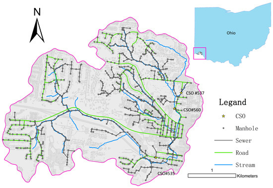
Figure 1.
Study area.
2.2. Design Storms
To investigate the sewer performance under different rainfall characteristics, 42 synthetic rainfall events with 10-min intervals are created with different durations, return periods, and locations of peak intensity by HydroCAD (Figure 2). The concentration time of the study area ranges around 0.44–1.8 hour. In reference to the Cincinnati Intensity Duration Frequency (IDF) curve, rainfall events are assorted by duration as short term and long term. Considering the sewer pipes reach their capacity at different speeds under various rainfall durations, the number of filled pipes induces complex sewer behaviour and influence. Hence, we select 2-h rainfall as a short-term event and 24-h rainfall as a long-term event to investigate the dynamic hydraulic behaviour of the sewer system. The two groups have different locations of peak value (early peak, middle peak, and late peak). According to rainfall duration and peak position, we group these events as 2-0.5, 2-1, 2-1.5, 24-4, 24-12, and 24-20. Moreover, each group contains seven return periods (1-year, 2-year, 5-year, 10-year, 25-year, 50-year, and 100-year).
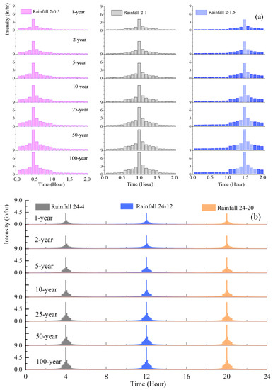
Figure 2.
Synthetic rainfall distributions: (a): 2-h event, (b): 24-h event.
2.3. Performance Measurements
Measurements of the integrated behaviour involve the road network and sewer network. Given the coupled topological structure of the two systems, we adopt the complex network method to assess the integrated behaviour. The operational part is measured by the functional components (FF) when some network components are damaged or malfunctioning during rainfall:
where t is the time of damage to the network, Nt is the number of functional components at time t, and N is the total number of components.
In addition, connectivity is the basis of network robustness, and FF only shows the state of a single component rather than the performance of the entire network. Hence, based on network science, the number of connected functional components (also called a giant component) within networks is defined as efficient clusters when the network is damaged [2,51,52]. The size of the giant component (FG) is used as an index of the network robustness and calculated as:
where Gt is the number of components in the giant component at time t. We employ different indicators to represent the performance of the two systems. For the sewer network, the depth ratio (d/D) is the crucial index of the hydraulic load of the sewer pipe. A pipe malfunction occurs when its d/D is above a threshold. We calculate the distribution of design parameters contained in the CAGIS dataset, and the distribution shows that more than 94% of pipes reach the maximum design flow when d/D ≥ 0.6. Additionally, the part-full pipes contain sediment and gas during regular operation, and the maximum flow rate occurs when d/D = 0.81 based on the calculation of part-full pipe flow [53]. Hence, we assume that 0.6 is the boundary condition for sewer pipe capacity. For the road network, we use the height of surface flow to determine the state of the road. The state of the road section consists of two types: connected with the road network and disconnected from the road network. Based on the Cincinnati road design manual, the curb height is set to 0.15 m [54]. Moreover, the overflow may lead to the vehicle rerouting and being trapped. Therefore, we assume the road section is disconnected from the adjacent road network when the overflow height exceeds 0.15 m. The FG is calculated according to the value of d/D and the road state. Thus, the components of FG consist of an interconnected operative sewer pipe (d/D < 0.6) and connected road (overflow height < 0.15 m), and these two parts are also mutually interconnected in FG. The above calculation is carried out in MATLAB, and the number of FG is calculated every minute with the rainfall process.
2.4. Identify Critical Pipes
According to the above calculation of FG, we calculate the statistics of the pipes that lead to the disintegration of the sewer network. However, not all pipes with a dramatic drop in FG would be identified as critical components. We select and locate critical pipes also based on the principle of inducing the network disconnect and the number of occurrences is over four times in every group, which means that these pipes appear in at least half of the simulation scenarios.
2.5. Scenario Development
Four simulation scenarios are developed, which are the baseline scenario, pipe enlargement scenario (PE), rain garden scenario (GI), and the combination of pipe enlargement and rain garden (GI + PE). Moreover, the reduction rate of road inundation is used to evaluate the effectiveness of control measures. The road section is marked as inundation when the height of overflow exceeds 0. We use the small threshold to avoid the unfairness assessment of the control measure effect. For example, if the overflow depth is 0.1 m before the control measure construction, the overflow depth is 0 after the construction. The control measure will be considered invalid when the threshold is 0.15 m. The baseline scenario represents the current situation of road inundation and sewer performance. By identifying critical pipes, we locate the components that significantly influence the performance of the whole sewer network. To improve the transportation efficiency of the sewer network, the diameter of the critical pipes doubles in the PE scenario. The total number of pipe enlargements is 91, and the average length is around 61.2 m. This scenario aims to reduce the vulnerability of the system and enhance global performance by improving the structure of local components. The rain garden is set in the sub-catchments of critical pipes and assumed to occupy full corresponding sub-catchments. The area of GI implementation accounts for approximately 28% of the total study area. The size of every rain garden is followed by sub-catchment property. A total of 114 sub-catchments have implemented GI facilities—the average area is 0.015 Km2, the average slope is 10.79, and the average value of the impervious area is around 30%. According to the SWMM manual, the percentage of impervious/pervious area treated is ignored if the LID practices occupy the whole sub-catchment. Since this study is mainly to determine whether mitigation measures can be implemented by identifying the location of critical pipes, the parameters refer to the default values in the SWMM manual. Relevant parameters are shown in Table 1 and Table 2. Pipe enlargement and rain gardens are set in the combination scenario, and the implementation of these two schemes follows the location of critical pipes.

Table 1.
Parameters of the rain garden.
Table 2.
Parameters of the pipe enlargement.
3. Results and Discussion
3.1. Sewer Network Performance under Different Rainfalls
To illustrate sewer behaviour under different rainfall patterns, Figure 3 plots the functional pipes (FF) and giant components (FG) of the sewer network under different peaks and return periods of short-term rainfall events (2-0.5, 2-1, and 2-1.5). FF and FG decrease significantly with increasing rainfall, and the decrease in FG is more severe than that in FF. We can see that FG drops to the lowest value, while more than 50% of pipes are not overloaded. Moreover, the variation in FG is quite different from that in FF, the number of overloaded pipes increases as the rainfall increases, and the minimum value of FF decreases continuously. However, FG directly decreases to a lower level, and the minimum value of FG is stable. In terms of the peak position, the location of the rainfall peak has a more prominent effect on FF than FG. FG reaches the lowest value before the peak arrives, and the minimum value of FF appears after the rainfall peak in all simulation events. Therefore, although the speed of pipe overload becomes slower with the delay of the rainfall peak, the disconnection of the whole sewer network is not delayed. Inevitably, the time of FG staying at the lowest level becomes longer with increasing rainfall. Hence, the sewer network needs a longer time to regain connections and recover the conveyance efficiency. However, the number of overloaded pipes does not display this situation since the FF gradually rises after rainfall, implying that most pipes recover their capacity. As a result, the recovery pipes are not connective in the function, and the whole sewer system operates at a lower performance.
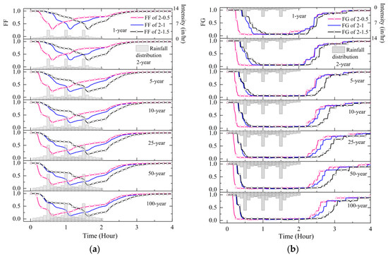
Figure 3.
The variations in the values of the fractions of FF and FG in different rainfall patterns. (a) FF, (b) FG. The grey histogram is the rainfall distribution, the pink curve with triangles is the 2-0.5 event, the blue line is the 2-1 event, and the black line with squares displays the 2-1.5 event.
In terms of long-term rainfall events, the change process of FF is similar to that of short-term rainfall when leaving out the peak position. FF decreases slowly at the beginning of rainfall and sharply drops as rainfall approaches the peak value, and the minimum value of FF appears after the peak (Figure 4). However, FG displays different trends. The decrease in FG is still faster than that of FF, but it does not directly drop to the minimum value. FG drops dramatically to a lower level at short-term events and remains at the value until the end of the rainfall. For long-term events, especially in small rainfall events (e.g., less than 10-year events), FG falls step by step. With rainfall development, FG first decreases to approximately 0.4 and drops to the lowest value when the rain peak occurs. Combined with the rainfall peak value, the peak position significantly impacts FG and the falling speed of FF. Under the same rainfall amount, the later the rainfall peak appears, the slower the decreasing speed of FG is. When the rainfall begins to weaken, both FF and FG recover gradually. Unlike short-term rainfall events, the peak position has a more notable effect on the recovery of FF rather than FG since FG remains at a low value until the end of the rainfall. Nonetheless, FG begins to rise after the rainfall peak in the long-term rainfall.
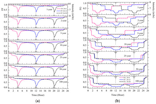
Figure 4.
The variations in the values of the fractions of FF and FG in different rainfall patterns. (a) FF, (b) FG. The grey histogram is the rainfall distribution, the pink curve with triangles is the 24-4 event, the blue line is the 24-12 event, and the black line with squares displays the 24-20 event.
The trend of the FF curve indicates the state of individual pipes under different rainfall patterns. The sewer pipe reaches capacity as the rainfall increases, and the number of overloaded pipes rises with the increase in the return period. Additionally, the location of the rainfall peak has a notable influence on FF, and the number of functional pipes decreases to the minimum as the rainfall reaches the maximum. This result is similar to Chen et al. [55]—for the same return period in short-term events, the later the peak arrives, the longer the pipe malfunction lasts. Moreover, we also find that the earlier peak arrives, the longer it takes for the pipe to recover capacity in short-term events. However, FF only reflects the performance of the single pipe rather than the behaviour of the entire sewer network. FG profiles the state of the sewer system, and the results show that the entire sewer network is significantly different from individual behaviour under different rainfall patterns. Compared with long-term events, the sewer network has the worst connectivity in short-term rainfall events. We can see in Figure 3b and Figure 4b that FG drops to the lowest value within half an hour of rainfall, and the whole sewer network becomes separated. At that time, peak rainfall does not occur, and half of the pipes are not overloaded. In long-term rainfall, the connectivity of the sewer network is better. For the same rainfall amount, the connectivity of the sewer network presents slower stepwise decline if the peak value appears later. Furthermore, FG shows that the recovery of the sewer system is faster under long-term rainfall since FG gradually begins to climb as the rainfall declines. Nevertheless, FG begins to recover until rainfall ends in short-term rainfall events. Given that FG reflects the connectivity and transportation efficiency of the entire sewer network, short-term rainfall events are more destructive and have a more adverse impact on the performance of the sewer system.
3.2. Identification of Critical Pipes
We observe several dramatic plummets (Figure 3b and Figure 4b) in the FG curves, which induce the whole network to split. In all scenarios, more than 200 pipes are identified to cause the dramatic drop in FG. Finally, we recognise the 92 common pipes where the number of occurrences is over half from 42 rainfall events. These common pipes are assumed as the common critical pipes of the entire network, since the state of these pipes has a notable impact on the sewer system behaviour. Figure 5 displays the distribution of the common critical pipes. Most of the critical components are trunk pipes, which are mainly responsible for collecting water of multiple branch pipes. It is worth noting that these critical pipes are indeed difficult to identify by general methods since they have the same size as the adjacent pipes, and the corresponding slope is not very steep. Hence, there is no significant difference between the critical pipes and their adjacent pipes, except for very few exceptions, meaning the impact is easily omitted. Therefore, based on the location of critical pipes, we determine the GI locations and pipes that need to be retrofitted. Notably, a few branch pipes are critical pipes. To avoid the diameter of branch pipes being larger than the trunk pipes, we do not enlarge the size of branch pipes in the PE scheme. Instead, we set up a rain garden in the corresponding sub-catchments of these branch pipes in GI and GI + PE projects.
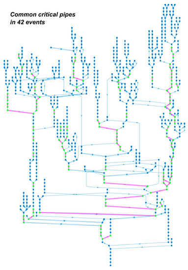
Figure 5.
Distribution of critical pipes. Red edges are the critical pipes, and green nodes are the manholes connected to the critical pipes.
3.3. Road Inundation in the Baseline Scenario
The road inundation under different rainfall patterns is shown in Figure 6, including short-term and long-term groups. The amount of rainfall significantly influences inundation, and inundated roads rise with the increase in rainfall. There is no doubt that heavy rainfall causes more serious road inundation. Nevertheless, a long duration of rainfall does not cause more severe consequences. Compared with road inundation under short-term and long-term events, the number of inundated roads is more significant in the short-term rainfall, and the submergence duration is longer. Additionally, the peak value also has a notable impact on road inundation, whether in short-term or long-term events. Although the maximum value of inundated roads appears after the rainfall peak, the inundation rises at a completely different rate. The road inundation rises immediately as the rainfall peak arrives and decreases after a peak value in long-term events, and mainly concentrates around the rainfall peak and lasts about 2 h. In short-term events, the inundated roads are close to 50% before peak rainfall. After the peak value, road inundation begins to decline, but the rate is much slower than long-term events. Until the end of rainfall, the inundation has not entirely subsided. Moreover, for the same return period rainfall, the inundated roads have the fastest rising rate in the early peak event. Nevertheless, this situation does not appear in long-term events. Sewer performance can explain why short-term events cause severe inundation. Combined with the change in FG (shown in Figure 3b and Figure 4b), FG drops to the bottom quickly as a number of pipes are filled in short-term rainfall events, which indicates that the entire sewer network is disconnected. The separated sewer network cannot cope with extensive rainfall, resulting in a dramatic increase in road inundation. However, although FG drops sharply in long-term rainfall events, the value does not drop to the bottom level directly. Instead of falling apart, the entire sewer network is separated into several sub-networks that still function effectively before the peak value arrives. Therefore, road inundation is not as severe as that in short-term events.
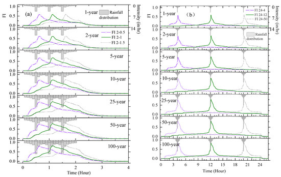
Figure 6.
The variations in the fraction of road inundation in different rainfall patterns. (a) 2-h event, (b) 24-h event. The grey histogram shows the rainfall distribution, the purple curve with triangles indicates 2-0.5 and 24-4 events, the green lines indicate 2-1 and 24-12 events, and the dotted lines indicate 2-1.5 and 24-20 events.
3.4. Retrofit Effect
The reduction rate of inundated roads is used to investigate the retrofitting effect. For short-term rainfall, Figure 7 shows the effect of GI, PE, and GI + PE under different rainfall patterns. Overall, PE is the least effective, and the performances of GI and GI + PE are better than PE. The function of the three mitigation measures gradually weakens with the increase in the return period. Especially in the 50-year and 100-year events, pipe retrofitting has little effect. The effect of mitigation measures is also affected by the time of the rainfall peak. At the beginning of rainfall, the three measures can reduce the amount of road inundation. GI can decrease road inundation by more than 50% during the first half-hour of rainfall. As rainfall increases, the capacity of mitigation measures gradually decreases. When the rainfall peak occurs, all three measures are almost invalid, and the number of flooded roads is the same as that of the baseline. GI and PE can alleviate road inundation with the decline in rainfall again, but this situation is not apparent under 50-year and 100-year events. For long-term rainfall, the control measures with GI perform better than those in short-term rainfall. The GI scheme lessens road inundation by more than half, except in a few cases (Figure 8). In contrast, the PE scheme is almost ineffective and worse than that under short-term conditions. Similar to short-term events, the influence of GI and GI + PE measures is limited when the rainfall is at a maximum. As the rainfall peak arrives, the number of inundated roads gradually increases. Therefore, peak position has a significant impact on the function of mitigation measures. Although the GI capacity diminishes slightly with the increase in the return period, the performance of GI in long-term events is more satisfactory than that in short-term events.
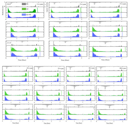
Figure 7.
The fraction of road inundation reduction in different rainfall patterns of short-term events. The dark grey area is the scheme of pipe enlargement (PE), the green area is the GI scheme, and the blue area is GI + PE.
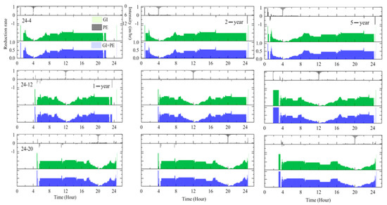
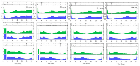
Figure 8.
The fraction of road inundation reduction in different rainfall patterns of long-term events. The dark grey area is the scheme of pipe enlargement (PE), the green area is the GI scheme, and the blue area is GI + PE.
The three schemes can reduce road inundation, but at different magnitudes, and the GI scheme has the best performance in this study. Among the project types, the average reduction in road inundation by GI and GI + PE is approximately 10% in short-term events, while that of PE is only approximately 2% (Table 3). GI and GI + PE perform better under long-term events, and the reduction average of these two projects is over 30% in group 24-4 (Table 4). For the rest of the scenarios (24-12 and 24-20), the average reduction value of GI and GI + PE is close to 30%. The effect of PE is still not significant, with a reduction average of less than 1%, even worse than that under short-term rainfall. In addition, the current results do not explain a clear relationship between PE performance and rainfall patterns since the trend of reduction fluctuated in all PE simulations. Moreover, comparing the road inundation of short-term events and long-term events illustrates that GI can adequately cope with long-term rainfall. According to the analysis of pipe behaviour in Section 3.1, short-term rainfall causes local pipes to reach capacity immediately and induces the disintegration of the entire sewer network. Therefore, GI does not have adequate time to collect a large amount of rainfall, which leads to severe inundation. In terms of long-term rainfall, although the rainfall lasts for a long time, the disintegrated sewer system becomes several sub-networks. GI can cooperate with sub-networks to maintain transportation efficiency and has enough time to reduce runoff generation. Previous studies confirmed that GI had a better effect on short-duration and frequent rainfall events [9]. However, we found that combining GI projects with sewer behaviour can also obtain a preferable effect in long-duration rainfall.
Table 3.
Average reduction rate of road inundation in short-term events.
Table 4.
Average reduction rate of road inundation in long-term events.
The results show that the synergistic relationship between GI and the sewer system is complicated, with limited recognition. The synergistic effect among various urban water infrastructures is confirmed by investigating the performance of different LID facilities [50]. However, the drainage system performance is treated as static in that investigation. Our study displays the dynamic behaviour of sewer systems and the influence between local component behaviour and system performance. The results show that sewer behaviour is complicated and dynamic during rainfall, depending on the rainfall pattern, interaction among components, and dynamic inflow. The GI outflow is critical since GI reduces the runoff generation and the sewer pipe inflow. The combined effect between sewer behaviour and GI performance will also lead to different control effects. Therefore, it can be found that it is reasonable to determine GI and the sewer update plan combined with the sewer behaviour. The results may contribute to understanding the combined relationship between sewer behaviour and GI performance. However, the results should be applied with caution in other cases since the drainage pattern is not the same (e.g., combined or separate system). Additionally, we can see that in all the simulations, the PE schemes seem to have little effect on alleviating road inundation, which is mainly caused by the following reasons. First, some critical pipes are distributed independently, and enlarging the diameter of certain critical pipes without a relevant retrofit plan of adjacent pipes cannot achieve the expected effect. In other words, simply expanding a single component can only increase storage space, which is a local effect and very small. After all, rather than water storage, the function of the sewer system is an effective conveyance. Second, we do not analyse the sewer network performance after enlarging the pipes. Updating the size of some pipes in the sewer system may produce new hydraulic characteristics, which may cause the phenomenon of new inundation or a bottleneck effect, inducing excessive water accumulation in the critical pipes. In addition, expanding the diameter of specific pipes in the network may reconstruct the topology structure of the network, resulting in the fluctuation of hydraulic behaviour and instability of the PE effect. However, this phenomenon is indeed impressive and worthy of further study.
4. Conclusions
Green infrastructure is implied based on sewer network behaviour to mitigate urban inundation and understand the interaction between the sewer system and GI projects. The critical components of the sewer system are identified by investigating 42 design rainfall events with different return periods, peak positions, and durations. Given these critical pipes, various green and grey infrastructure schemes are designed for risk reduction and stormwater management.
The results reveal that the local pipe behaviour has a diverse influence on the sewer network. The overload of the critical pipes leads to a significant reduction in system performance, which means that appropriate retrofits aimed at the critical parts can make up for the weak connectivity of the sewer network and systematically improve the sewer conveyance capacity. The three retrofits are used in this study to reduce road inundation, and the different effects highlight the interaction between the sewer behaviour and retrofits. Among them, the effect of PE is the weakest; the GI and GI + PE performances are satisfactory. However, GI + PE may need additional costs, implying that GI is the optimal scheme in this study. The mitigation consequences confirm that although it is feasible to locate a retrofit program by identifying critical components, inappropriate measures have little effect. The PE retrofit increases the volume of critical pipes, but the effect is local, and single pipe enlargement may rebuild the topology of the drainage system. Thus, GI projects perform better since GI further enhances the sewer system connectivity besides controlling the inflow of sewer pipes. In addition to the sewer behaviour, the mitigation performance is affected by rainfall patterns. For short-term rainfall, the influence of peak position is limited. GI-based projects present better in the middle and late peak events than in the early peak. For long-term events, peak position has a significant influence since GI-based retrofits can significantly alleviate inundation except for peak times. Therefore, local pipes cause system performance reduction, but the improvement plan may be beyond the specific structural promotion. Sewer behaviour and GI performance are dynamic interactions and are affected by rainfall patterns. The retrofit scheme should be targeted at vulnerable parts of the drainage network, but the topology feature of the system should be treated carefully. Consequently, the mitigation measures should correspond to the local rainfall characteristics and sewer behaviour to achieve better stormwater management in actual practice.
Our proposed approach provides a new view for green infrastructure implementation and evaluating sewer system performance. For urban areas, the high density of the built environment limits GI space availability, and ageing facilities make renovation challenging. It is necessary to combine sewer behaviour with GI to optimise planning and updating. Although the PE scenario has a limited effect in our research, this scheme is essential for other sewer system retrofits. In addition, we notice that the GI effect is not significant during the rainfall peak period. We only adopt rain gardens as the representative GI in this study. A number of studies have shown that the combination of various green infrastructure options may lead to different effects [18,19,22]. Therefore, different GI types, combinations, and comprehensive index assessments will be tried in future research. Furthermore, the proposed approach can also be extended in related fields, for instance, taking the dynamic traffic flow with inundated roads for rerouting and avoiding vehicles trapped in floods.
Author Contributions
C.S.: Conceptualization, Methodology, Software, Validation, Data curation, Writing—original draft, Writing—review and editing, Visualization. H.X.: Funding acquisition. X.F.: Resources, Writing—original draft, Writing—review and editing. X.W.: Conceptualization, Validation, Writing—original draft, Writing—review and editing, Visualization. W.W.: Writing—review and editing. All authors have read and agreed to the published version of the manuscript.
Funding
This study was supported by the scholarship from China Scholarship Council (CSC.201807090031).
Institutional Review Board Statement
Not applicable.
Informed Consent Statement
Not applicable.
Data Availability Statement
Not applicable.
Acknowledgments
We would like to thank the Cincinnati Area Geographic Information System and the Metropolitan Sewer District of Greater Cincinnati for the data support. We also thank the reviewers for their valuable suggestions to improve this paper.
Conflicts of Interest
The authors declare no conflict of interest.
Appendix A
Appendix to this article can be found online at:
Integrated Model
The integrated model consists of the road–sewer interaction system, the road network and sewer network are abstracted, respectively, and the two systems are connected through a manhole based on geographical interdependency. The hydraulic characteristics of the integrated model include overland flow, channel flow (road network), sewer flow, and stream flow. Sewer overflow from manholes is input to the road network, and water on the road network returns to the sewer network through manholes. The integrated model is implemented by the Stormwater Management Model (SWMM).
The sewer network and stream network
The sewer network model follows the actual drainage layout and component properties, and the sewer lines are generalised as pipes. We model streams with variable cross-sectional shapes derived from the Digital Elevation Model data (DEM) and set them as customised channels with virtual nodes in the model. The virtual nodes are set in the bifurcation point, confluence point, and point of flow direction change. Node elevation is extracted from DEM. Both networks use Saint-Venant equations to simulate flow. The inflows of the sewer system and stream are the outflows of corresponding sub-catchments. We delineate sub-catchments by the D8 algorithm of ArcGIS according to the surface features and stream/sewer network location.
Road network
The entire road network creates open channels in SWMM, and the cross-section is customised as an irregular shape. The roads are set as a diverted conduit of sewer pipes, and manholes are treated as the linkage. Thus, the excess flow will be discharged to the road network through manholes when the sewer pipe reaches capacity. Therefore, we use dividers to replace the manholes that connected the road and sewer, and the rest of the manholes are modelled as nodes in the SWMM. The kinematic wave is adopted in the runoff calculation. The relevant parameters are defined by the SWMM manual and published literature [56]. Additionally, the initial flow width, sub-catchment area, and the longest flow path are determined individually using ArcGIS.
Model calibration and validation
Historical rainfalls are used for model calibration and validation. Simulation results are evaluated by the coefficient of the Nash–Sutcliffe (Equation (A1)) efficiency (NSE) coefficient [57]. The parameters are calibrated by comparing the simulation with monitored data of CSO #537. CSO #535 ends at a depression area and does not connect with the stream. Additionally, monitoring data show CSO #560 barely has outflow during heavy rainstorms, and CSO #537 is the only outlet discharging directly to the stream. Hence, CSO #535 is modelled as the pipe end, the overflow water level of CSO #537 is used for calibration and validation, and the overflow events of CSO #560 are adopted for validation. The simulation results are compared with monitoring data every 5 min since the water level of CSO #537 is recorded every 5 min. The NSE ranges (Table A1) are used to evaluate the simulation results: the value ranges from −∞ to 1; in general, the closer the value is to 1, the more reliable the model is [58,59]. Furthermore, by comparing the frequency of overflow events of CSO #560, we conduct a long-term simulation as another validation of the model.
where is the monitored value at time t, is the simulated value (in) at time t, and is the average for the monitored value (in).
Table A1.
NSE range.
Table A1.
NSE range.
| NSE | Model Performance |
|---|---|
| 0.75 < NSE < 1 | Very good |
| 0.65 < NSE < 0.75 | Good |
| 0.5 < NSE < 0.65 | Satisfactory |
| NSE ≤ 0.5 | Unsatisfactory |
| NSE < 0 | Not credible |
The calibration parameter is shown in Table A2. Given that the study area adopts a combined drainage regime, we use the pipe flow data in clear days to estimate the average water level in the CSO #537 outlet. Two rainfall events (C1:18 July 2016 and C2: 8 July 2016) are used as calibration, and the NSE values are 0.855 and 0.813, respectively (Figure A1). The validation results are shown in Figure A2, using storms V1 (17–18 May 2016) and V2 (10 September 2016). The NSE values are 0.73 and 0.70, respectively, showing that our model has sound performance. We note the differences between the simulated and the measured data, and the domestic sewage discharged may result in a slight flow difference. Moreover, DEM data for the urbanised area may also introduce errors. The verification of CSO #560 includes five groups, namely June 2014, September 2015, August 2016, June 2017, and July 2017. In the validation process, all rainfall events in the whole month are taken as the input of SWMM, and the simulation time is from the first day to the last day of the month. Finally, the date of the overflows is marked and compared with the records (Table A3). The results show that the simulated overflow date matches the recorded date, although there is a slight difference. This difference is mainly due to the recording error. According to the rainfall records, heavy rainfall occurred on 7/7/2017 and 6/18/2017, and the overflow events also appeared in CSO #537. Therefore, this slight difference is mainly caused by the records. Based on the NSE range and the records of overflow events, the validation results are satisfactory, and the integrated model is capable of research.
Table A2.
The parameters of the integrated model.
Table A2.
The parameters of the integrated model.
| Parameter | Category | Calibration Value | Calibration Interval/Design Parameter |
|---|---|---|---|
| Manning’s roughness coefficient | Storm conduits Pipe Street Stream | 0.022 0.015/0.017 0.017 0.04 | 0.022 0.011–0.026 0.011–0.035 0.03–0.07 |
| Manning’s N | N-Imperv N-Perv | 0.011 0.11 | 0.011–0.015 0.06–0.41 |
| D_storage | Impervious Pervious | 0.1 0.3 | 0.05–0.1 0.1–0.3 |
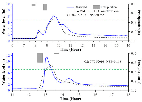
Figure A1.
Model calibration.
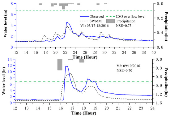
Figure A2.
Model validation.
Table A3.
Validation results from overflow events of CSO #560.
Table A3.
Validation results from overflow events of CSO #560.
| Time | Overflow Records | Simulation Results |
|---|---|---|
| June 2014 | 6/4/2014 | 6/4/2014 |
| September 2015 | 9/5/2015 | 9/5/2015 |
| August 2016 | 8/15/2016 8/17/2016 8/28/2016 | 8/15/2016 8/17/2016 8/28/2016 |
| June 2017 | 6/23/2017 | 6/23/2017 6/18/2017 |
| July 2017 | 7/13/2017 | 7/13/2017 7/7/2017 |
References
- Mohanty, M.P.; Mudgil, S.; Karmakar, S. Flood Management in India: A Focussed Review on the Current Status and Future Challenges. Int. J. Disaster Risk Reduct. 2020, 49, 101660. [Google Scholar] [CrossRef]
- Wang, W.; Yang, S.; Stanley, H.E.; Gao, J. Local Floods Induce Large-Scale Abrupt Failures of Road Networks. Nat. Commun. 2019, 10, 2114. [Google Scholar] [CrossRef]
- Hosseinzadehtalaei, P.; Ishadi, N.K.; Tabari, H.; Willems, P. Climate Change Impact Assessment on Pluvial Flooding Using a Distribution-Based Bias Correction of Regional Climate Model Simulations. J. Hydrol. 2021, 598, 126239. [Google Scholar] [CrossRef]
- Jha, M.; Afreen, S. Flooding Urban Landscapes: Analysis Using Combined Hydrodynamic and Hydrologic Modeling Approaches. Water 2020, 12, 1986. [Google Scholar] [CrossRef]
- Kourtis, I.M.; Tsihrintzis, V.A. Adaptation of Urban Drainage Networks to Climate Change: A Review. Sci. Total Environ. 2021, 771, 145431. [Google Scholar] [CrossRef]
- Arnone, E.; Pumo, D.; Francipane, A.; La Loggia, G.; Noto, L.V. The Role of Urban Growth, Climate Change, and Their Interplay in Altering Runoff Extremes. Hydrol. Process. 2018, 32, 1755–1770. [Google Scholar] [CrossRef]
- Skougaard Kaspersen, P.; Høegh Ravn, N.; Arnbjerg-Nielsen, K.; Madsen, H.; Drews, M. Comparison of the Impacts of Urban Development and Climate Change on Exposing European Cities to Pluvial Flooding. Hydrol. Earth Syst. Sci. 2017, 21, 4131–4147. [Google Scholar] [CrossRef] [Green Version]
- Zhou, Q.; Leng, G.; Su, J.; Ren, Y. Comparison of Urbanization and Climate Change Impacts on Urban Flood Volumes: Importance of Urban Planning and Drainage Adaptation. Sci. Total Environ. 2019, 658, 24–33. [Google Scholar] [CrossRef] [PubMed]
- Qin, H.; Li, Z.; Fu, G. The Effects of Low Impact Development on Urban Flooding under Different Rainfall Characteristics. J. Environ. Manag. 2013, 129, 577–585. [Google Scholar] [CrossRef] [PubMed] [Green Version]
- Babovic, F.; Mijic, A. The Development of Adaptation Pathways for the Long-term Planning of Urban Drainage Systems. J. Flood Risk Manag. 2019, 12, e12538. [Google Scholar] [CrossRef] [Green Version]
- Kang, N.; Kim, S.; Kim, Y.; Noh, H.; Hong, S.; Kim, H. Urban Drainage System Improvement for Climate Change Adaptation. Water 2016, 8, 268. [Google Scholar] [CrossRef] [Green Version]
- Casal-Campos, A.; Fu, G.; Butler, D.; Moore, A. An Integrated Environmental Assessment of Green and Gray Infrastructure Strategies for Robust Decision Making. Environ. Sci. Technol. 2015, 49, 8307–8314. [Google Scholar] [CrossRef] [PubMed] [Green Version]
- Zhou, Q. A Review of Sustainable Urban Drainage Systems Considering the Climate Change and Urbanization Impacts. Water 2014, 6, 976–992. [Google Scholar] [CrossRef]
- Barbosa, A.E.; Fernandes, J.N.; David, L.M. Key Issues for Sustainable Urban Stormwater Management. Water Res. 2012, 46, 6787–6798. [Google Scholar] [CrossRef]
- Chen, W.; Wang, W.; Huang, G.; Wang, Z.; Lai, C.; Yang, Z. The Capacity of Grey Infrastructure in Urban Flood Management: A Comprehensive Analysis of Grey Infrastructure and the Green-Grey Approach. Int. J. Disaster Risk Reduct. 2021, 54, 102045. [Google Scholar] [CrossRef]
- Pour, S.H.; Wahab, A.K.A.; Shahid, S.; Asaduzzaman, M.; Dewan, A. Low Impact Development Techniques to Mitigate the Impacts of Climate-Change-Induced Urban Floods: Current Trends, Issues and Challenges. Sustain. Cities Soc. 2020, 62, 102373. [Google Scholar] [CrossRef]
- Fu, X. Assessment of Green Infrastructure Performance through an Urban Resilience Lens. J. Clean. Prod. 2021, 11, 125146. [Google Scholar] [CrossRef]
- Chatzimentor, A.; Apostolopoulou, E.; Mazaris, A.D. A Review of Green Infrastructure Research in Europe: Challenges and Opportunities. Landsc. Urban. Plan. 2020, 198, 103775. [Google Scholar] [CrossRef]
- Eckart, K.; McPhee, Z.; Bolisetti, T. Performance and Implementation of Low Impact Development—A Review. Sci. Total Environ. 2017, 607–608, 413–432. [Google Scholar] [CrossRef]
- Venkataramanan, V.; Lopez, D.; McCuskey, D.J.; Kiefus, D.; McDonald, R.I.; Miller, W.M.; Packman, A.I.; Young, S.L. Knowledge, Attitudes, Intentions, and Behavior Related to Green Infrastructure for Flood Management: A Systematic Literature Review. Sci. Total Environ. 2020, 720, 137606. [Google Scholar] [CrossRef]
- Caparrós-Martínez, J.L.; Milán-García, J.; Rueda-López, N.; de Pablo-Valenciano, J. Green Infrastructure and Water: An Analysis of Global Research. Water 2020, 12, 1760. [Google Scholar] [CrossRef]
- Fu, X.; Hopton, M.E.; Wang, X.; Goddard, H.; Liu, H. A Runoff Trading System to Meet Watershed-Level Stormwater Reduction Goals with Parcel-Level Green Infrastructure Installation. Sci. Total Environ. 2019, 689, 1149–1159. [Google Scholar] [CrossRef]
- Seo, M.; Jaber, F.; Srinivasan, R.; Jeong, J. Evaluating the Impact of Low Impact Development (LID) Practices on Water Quantity and Quality under Different Development Designs Using SWAT. Water 2017, 9, 193. [Google Scholar] [CrossRef]
- Zhang, K.; Chui, T.F.M. A Comprehensive Review of Spatial Allocation of LID-BMP-GI Practices: Strategies and Optimization Tools. Sci. Total Environ. 2018, 621, 915–929. [Google Scholar] [CrossRef]
- Czemiel Berndtsson, J. Green Roof Performance towards Management of Runoff Water Quantity and Quality: A Review. Ecol. Eng. 2010, 36, 351–360. [Google Scholar] [CrossRef]
- Bliss, D.J.; Neufeld, R.D.; Ries, R.J. Storm Water Runoff Mitigation Using a Green Roof. Environ. Eng. Sci. 2009, 26, 407–418. [Google Scholar] [CrossRef]
- Mangangka, I.R.; Liu, A.; Egodawatta, P.; Goonetilleke, A. Performance Characterisation of a Stormwater Treatment Bioretention Basin. J. Environ. Manag. 2015, 150, 173–178. [Google Scholar] [CrossRef] [Green Version]
- Chapman, C.; Horner, R.R. Performance Assessment of a Street-Drainage Bioretention System. Water Environ. Res. 2010, 82, 109–119. [Google Scholar] [CrossRef] [PubMed]
- Jamali, B.; Bach, P.M.; Deletic, A. Rainwater Harvesting for Urban Flood Management—An Integrated Modelling Framework. Water Res. 2020, 171, 115372. [Google Scholar] [CrossRef] [PubMed]
- Autixier, L.; Mailhot, A.; Bolduc, S.; Madoux-Humery, A.-S.; Galarneau, M.; Prévost, M.; Dorner, S. Evaluating Rain Gardens as a Method to Reduce the Impact of Sewer Overflows in Sources of Drinking Water. Sci. Total Environ. 2014, 499, 238–247. [Google Scholar] [CrossRef] [PubMed]
- Roebuck, R.M.; Oltean-Dumbrava, C.; Tait, S. Whole Life Cost Performance of Domestic Rainwater Harvesting Systems in the United Kingdom: Cost Performance of Domestic Rainwater Harvesting Systems. Water Environ. J. 2011, 25, 355–365. [Google Scholar] [CrossRef]
- Soulis, K.X.; Valiantzas, J.D.; Ntoulas, N.; Kargas, G.; Nektarios, P.A. Simulation of Green Roof Runoff under Different Substrate Depths and Vegetation Covers by Coupling a Simple Conceptual and a Physically Based Hydrological Model. J. Environ. Manag. 2017, 200, 434–445. [Google Scholar] [CrossRef] [PubMed]
- Lee, J.G.; Borst, M.; Brown, R.A.; Rossman, L.; Simon, M.A. Modeling the Hydrologic Processes of a Permeable Pavement System. J. Hydrol. Eng. 2015, 20, 04014070. [Google Scholar] [CrossRef]
- Chopra, M.; Kakuturu, S.; Ballock, C.; Spence, J.; Wanielista, M. Effect of Rejuvenation Methods on the Infiltration Rates of Pervious Concrete Pavements. J. Hydrol. Eng. 2010, 15, 426–433. [Google Scholar] [CrossRef]
- Imran, H.M.; Akib, S.; Karim, M.R. Permeable Pavement and Stormwater Management Systems: A Review. Environ. Technol. 2013, 34, 2649–2656. [Google Scholar] [CrossRef] [Green Version]
- Kamali, M.; Delkash, M.; Tajrishy, M. Evaluation of Permeable Pavement Responses to Urban Surface Runoff. J. Environ. Manag. 2017, 187, 43–53. [Google Scholar] [CrossRef] [PubMed]
- Ahiablame, L.; Shakya, R. Modeling Flood Reduction Effects of Low Impact Development at a Watershed Scale. J. Environ. Manag. 2016, 171, 81–91. [Google Scholar] [CrossRef]
- Raei, E.; Reza Alizadeh, M.; Reza Nikoo, M.; Adamowski, J. Multi-Objective Decision-Making for Green Infrastructure Planning (LID-BMPs) in Urban Storm Water Management under Uncertainty. J. Hydrol. 2019, 579, 124091. [Google Scholar] [CrossRef]
- Mei, C.; Liu, J.; Wang, H.; Yang, Z.; Ding, X.; Shao, W. Integrated Assessments of Green Infrastructure for Flood Mitigation to Support Robust Decision-Making for Sponge City Construction in an Urbanized Watershed. Sci. Total Environ. 2018, 639, 1394–1407. [Google Scholar] [CrossRef]
- Gong, Y.; Chen, Y.; Yu, L.; Li, J.; Pan, X.; Shen, Z.; Xu, X.; Qiu, Q. Effectiveness Analysis of Systematic Combined Sewer Overflow Control Schemes in the Sponge City Pilot Area of Beijing. IJERPH 2019, 16, 1503. [Google Scholar] [CrossRef] [Green Version]
- U.S. Environmental Protection Agency (USEPA). Reducing Stormwater Costs through Low Impact Development (LID) Strategies and Practices; EPA 841-F-07-006; USEPA Nonpoint Source Control Branch: Washington, DC, USA, 2007.
- Randall, M.; Sun, F.; Zhang, Y.; Jensen, M.B. Evaluating Sponge City Volume Capture Ratio at the Catchment Scale Using SWMM. J. Environ. Manag. 2019, 246, 745–757. [Google Scholar] [CrossRef]
- Carter, J.G.; Handley, J.; Butlin, T.; Gill, S. Adapting Cities to Climate Change—Exploring the Flood Risk Management Role of Green Infrastructure Landscapes. J. Environ. Plan. Manag. 2018, 61, 1535–1552. [Google Scholar] [CrossRef] [Green Version]
- Palla, A.; Gnecco, I. Hydrologic Modeling of Low Impact Development Systems at the Urban Catchment Scale. J. Hydrol. 2015, 528, 361–368. [Google Scholar] [CrossRef]
- Jarden, K.M.; Jefferson, A.J.; Grieser, J.M. Assessing the Effects of Catchment-Scale Urban Green Infrastructure Retrofits on Hydrograph Characteristics: Hydrologic Effects of Catchment-Scale Green Infrastructure Retrofits. Hydrol. Process. 2016, 30, 1536–1550. [Google Scholar] [CrossRef]
- Carson, T.B.; Marasco, D.E.; Culligan, P.J.; McGillis, W.R. Hydrological Performance of Extensive Green Roofs in New York City: Observations and Multi-Year Modeling of Three Full-Scale Systems. Environ. Res. Lett. 2013, 8, 024036. [Google Scholar] [CrossRef]
- Wang, X.; Shuster, W.; Pal, C.; Buchberger, S.; Bonta, J.; Avadhanula, K. Low Impact Development Design—Integrating Suitability Analysis and Site Planning for Reduction of Post-Development Stormwater Quantity. Sustainability 2010, 2, 2467–2482. [Google Scholar] [CrossRef] [Green Version]
- Wang, W.; Yang, S.; Gao, J.; Hu, F.; Zhao, W.; Stanley, H.E. An Integrated Approach for Assessing the Impact of Large-Scale Future Floods on a Highway Transport System. Risk Anal. 2020, 40, 1780–1794. [Google Scholar] [CrossRef] [PubMed]
- Schifman, L.A.; Herrmann, D.L.; Shuster, W.D.; Ossola, A.; Garmestani, A.; Hopton, M.E. Situating Green Infrastructure in Context: A Framework for Adaptive Socio-Hydrology in Cities. Water Resour. Res. 2017, 53, 10139–10154. [Google Scholar] [CrossRef]
- Zeng, S.; Guo, H.; Dong, X. Understanding the Synergistic Effect between LID Facility and Drainage Network: With a Comprehensive Perspective. J. Environ. Manag. 2019, 246, 849–859. [Google Scholar] [CrossRef]
- Gao, J.; Buldyrev, S.V.; Stanley, H.E.; Havlin, S. Networks Formed from Interdependent Networks. Nat. Phys. 2012, 8, 40–48. [Google Scholar] [CrossRef] [Green Version]
- Ouyang; Min. Review on Modeling and Simulation of Interdependent Critical Infrastructure Systems. Reliab. Eng. Syst. Saf. 2014, 121, 43–60. [Google Scholar] [CrossRef]
- Butler, D.; Digman, C.; Makropoulos, C.; Davies, J.W. Urban Drainage, 4th ed.; CRC Press: Boca Raton, FL, USA, 2018. [Google Scholar] [CrossRef]
- City of Cincinnati. Street Restoration Manual. 2012. Available online: https://www.cincinnati-oh.gov/dote/permits-licenses/dote-resource-center/subdivision-development/subdivision-development-streets-manual/ (accessed on 15 May 2019).
- Chen, W.; Huang, G.; Zhang, H.; Wang, W. Urban Inundation Response to Rainstorm Patterns with a Coupled Hydrodynamic Model: A Case Study in Haidian Island, China. J. Hydrol. 2018, 564, 1022–1035. [Google Scholar] [CrossRef]
- Rai, P.K.; Chahar, B.R.; Dhanya, C.T. GIS-Based SWMM Model for Simulating the Catchment Response to Flood Events. Hydrol. Res. 2017, 48, 384–394. [Google Scholar] [CrossRef]
- Nash, J.E.; Sutcliffe, I.V. River Flow Forecasting through Conceptual Models. J. Hydrol. 1970, 10, 282–290. [Google Scholar] [CrossRef]
- Moriasi, D.N.; Arnold, J.G.; van Liew, M.W.; Bingner, R.L.; Harmel, R.D.; Veith, T.L. Model Evaluation Guidelines for Systematic Quantification of Accuracy in Watershed Simulations. Trans. ASABE 2007, 50, 885–900. [Google Scholar] [CrossRef]
- Santhi, C.; Arnold, J.G.; Williams, J.R.; Dugas, W.A.; Srinivasan, R.; Hauck, L.M. Validation of the Swat Model on a Large Rwer Basin with Point and Nonpoint Sources. J. Am. Water Resour. Assoc. 2001, 37, 1169–1188. [Google Scholar] [CrossRef]
Publisher’s Note: MDPI stays neutral with regard to jurisdictional claims in published maps and institutional affiliations. |
© 2021 by the authors. Licensee MDPI, Basel, Switzerland. This article is an open access article distributed under the terms and conditions of the Creative Commons Attribution (CC BY) license (https://creativecommons.org/licenses/by/4.0/).