Multi Frequency Isotopes Survey to Improve Transit Time Estimation in a Situation of River-Aquifer Interaction

Abstract

The Barthelasse alluvial aquifer is used to supply water to 180,000 inhabitants. The pumping field is located less than 200 m from the Rhône and is 100% fed by water from the Rhône, which makes it particularly vulnerable to any pollution from the Rhône. Between the Rhône and the pumping field is a Girardon unit, an arrangement that can be found regularly along the banks of the lower and middle reaches of the Rhône, and whose role is to stabilise the banks (alluvial deposits) and to facilitate river navigation. In order to know the transfer times between the Rhône and the pumping field, fortnightly monitoring was carried out over a hydrological year, as well as hourly monitoring during a flood in the winter of 2019. The Rhône shows a cyclicality in its isotopic signature with enrichment in heavy isotopes during the winter period, particularly during floods, and a depletion during the summer period. This variation is found well within the associated alluvial aquifer. The application of LPMs models showed that the average transfer time between the Rhône and the Girardon unit was 20 days and 50 days between the Rhône and the Barthelasse pumping. This study highlighted the importance of using several sampling frequencies to consider the diversity of hydrological situations. For the Rhône, event-based monitoring (flooding) proved to be relevant to account for isotopic variability throughout the year. This work also highlighted the impact of the disruption of hydraulic exchanges between the river and the water table caused by the presence of the Girardon unit in terms of the propagation of contaminants.

1. Introduction

In France, alluvial aquifers provide 45% of the volume of water used for drinking water and for agricultural and industrial uses and play an important ecological role through their hydraulic link with wetlands [1]. This strong contribution to the water supply is explained by a shallow depth and favourable hydraulic properties, which allow high flow rates to be obtained at low operating costs. However, in this configuration, the alluvial aquifers are also highly vulnerable to pollution.

To address the issue of pollutant transfer, it is common to use natural or artificial tracing methods. In particular, the stable isotopes of the water molecule (²H, ¹⁸O) have many applications, allowing a better understanding of hydrosystems. They are used to estimate the recharge, to know the origin of water, the mixing processes and the transit times [2,3,4,5,6,7,8,9,10,11]. The use of this tracer is particularly relevant in the context of short transit times within the aquifer, as is the case for exchanges between alluvial aquifers and rivers. However, it is necessary to have a marked isotopic signature for the input signal to the system and a different signature between the input and output signal [11].

From continuous monitoring of the input signal, the average transit time between the river and the water table is deduced from a transfer model chosen a priori and from a calibration on the output concentrations. This method of LPM models is widely used in the field of isotopic hydrogeology in order to understand the age distribution of groundwater in the aquifer [12]. Although these models do not require detailed hydrogeological information, they provide a first understanding of the system and are locally relevant. In the case of the water table–river relationships, the results of these models allow a first approach of the aquifer transport parameters and have shown their interest in the simulation of mass transport [13], for the assessment of the vulnerability of groundwater to anthropogenic pollution [14] or to understand the sources of contaminants [15].

Several studies have also demonstrated the value of continuous monitoring of physicochemical parameters in situ, such as temperature and electrical conductivity, to determine transit times [16,17,18,19,20] and the relationships between surface water and groundwater [21,22,23,24]. By its lower cost compared to usual tracing methods, the use of these parameters allows very high-frequency monitoring. For the interpretation of the results, several approaches have been used, namely dynamic cross-correlation [19], the calibration of an advective-dispersive model [25] and parametric/non-parametric deconvolution [17].

The alluvial water table of the Rhône constitutes the major resource for supplying drinking water to the populations of the Rhône valley and its surroundings. In this region, in economic and demographic expansion, the pressures of occupation of space are increasing rapidly, which represents a risk of degradation of water quality and failure of the supply of drinking water from the alluvial corridor [26]. The present study concerns a pumping field located on the fluvial island of Barthelasse in Avignon (south-eastern France). It contributes to the drinking water supply of 180,000 inhabitants, and because of its proximity to the Rhône (<200 m) it is important to assess the potential impacts of the river on the contamination of groundwater in order to implement a strategy for resource protection.

Based on a 2-year isotopic survey of the various water masses and high-frequency physico-chemical monitoring in the Rhône and the groundwater, the main objective of this study is to propose, through a multi-method approach, a solid estimate of transit time between the Rhône and the pumping field. For this, the choice of the sampling frequency and the impact of the hydrological context will be assessed. A reflection will also be carried out on the optimisation method for estimating the model’s parameters and the consequences of this choice on the results. Finally, a comparison between the results from two independent tracers will be carried out in order to strengthen the conclusions in terms of vulnerability.

2. Materials and Methods

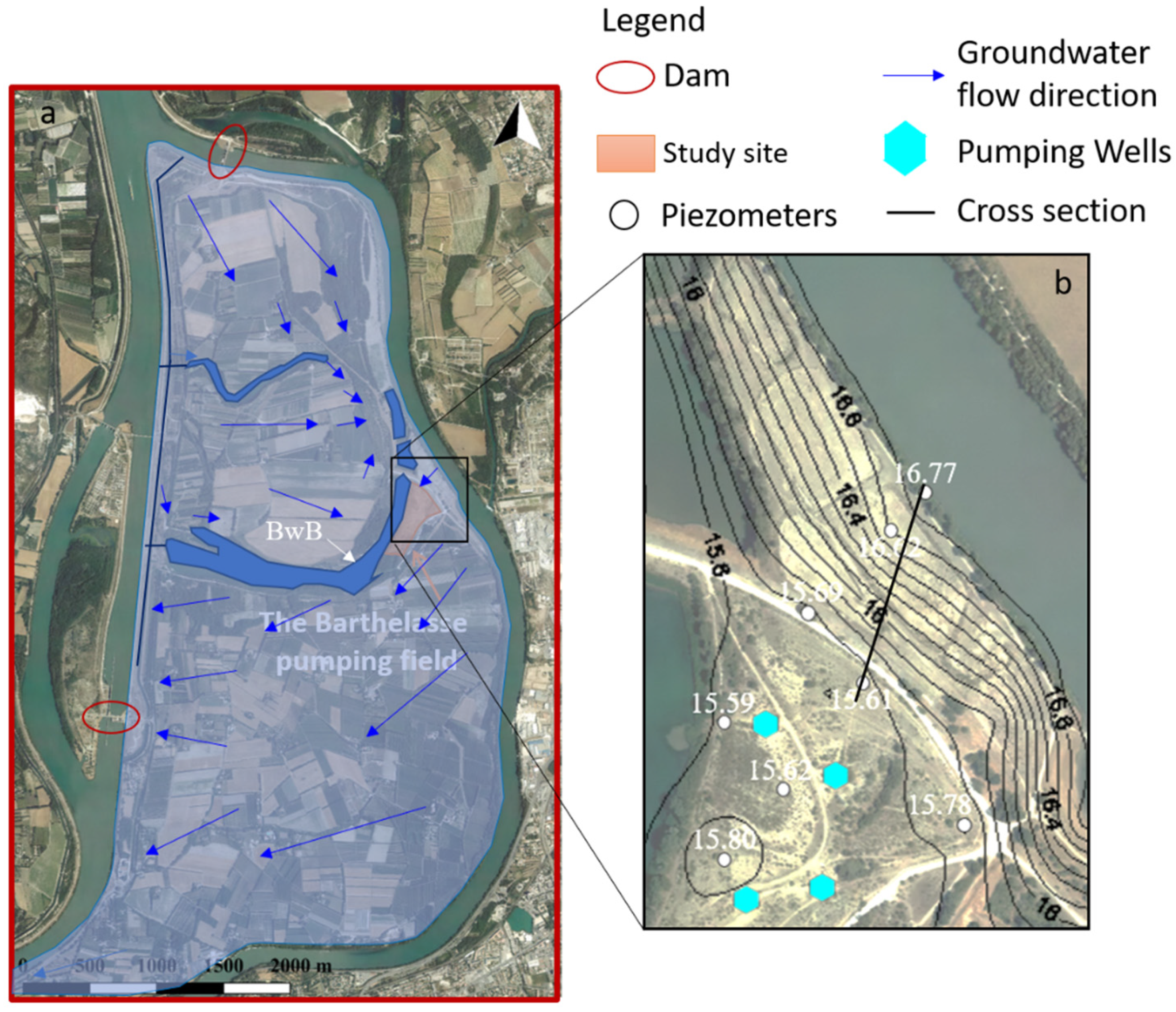
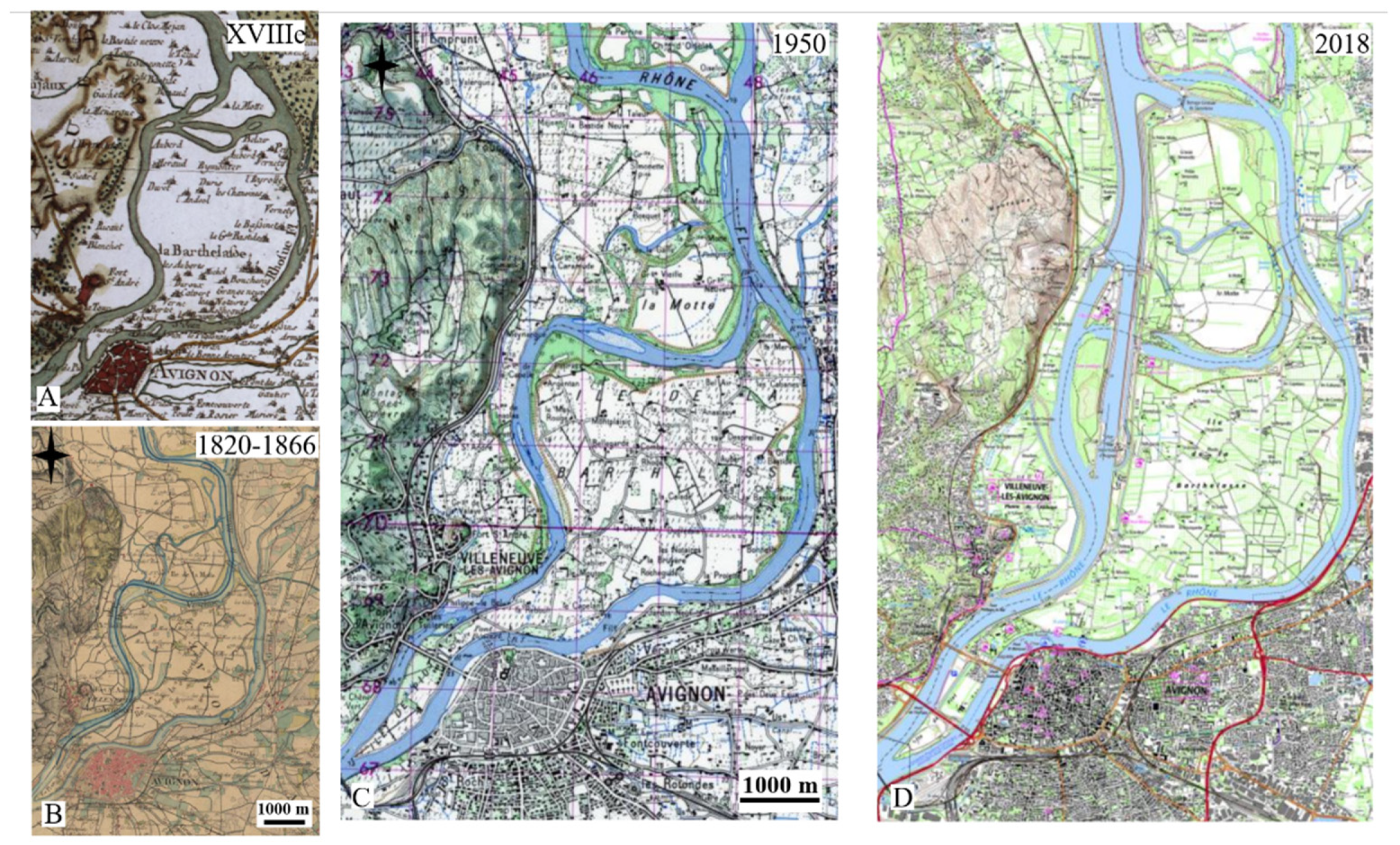
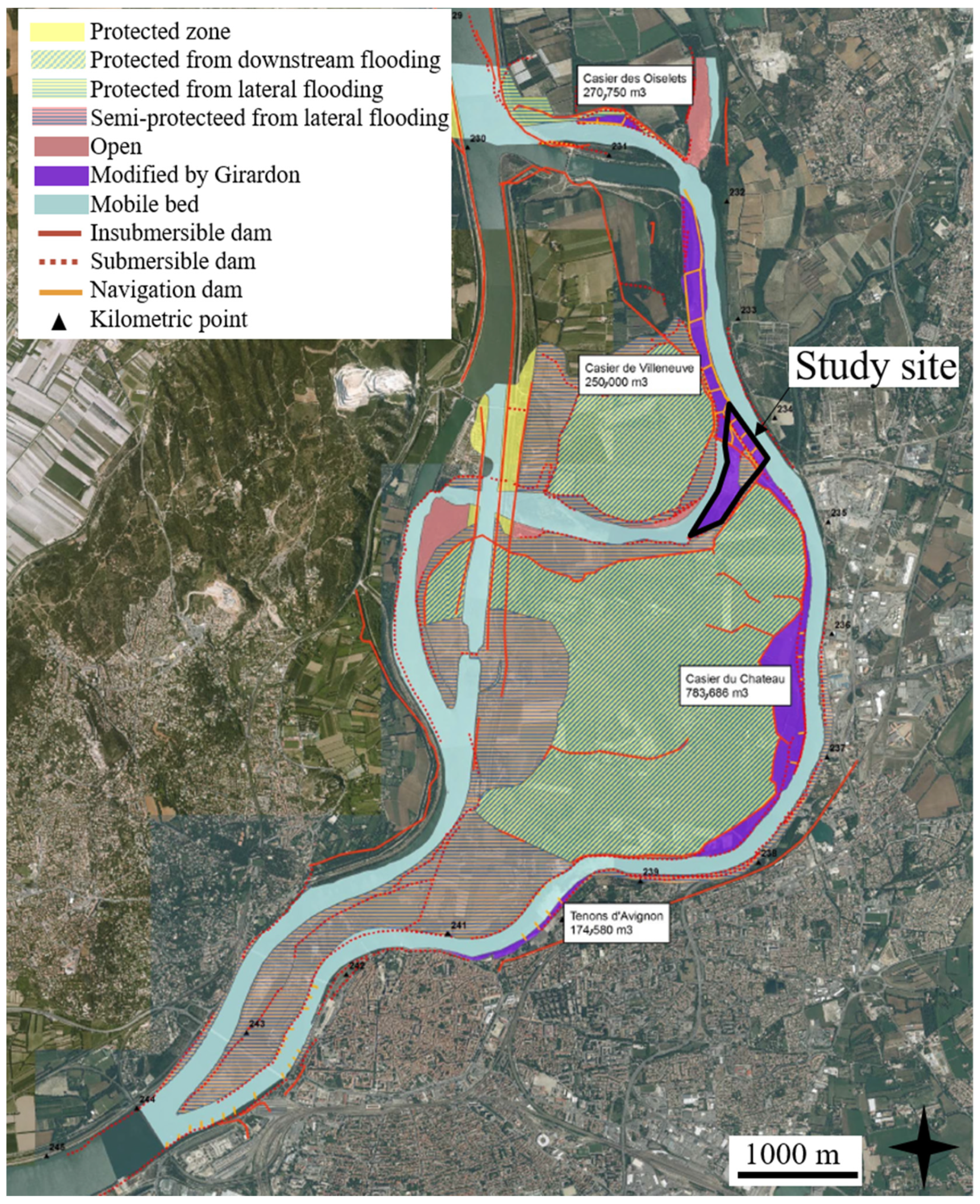
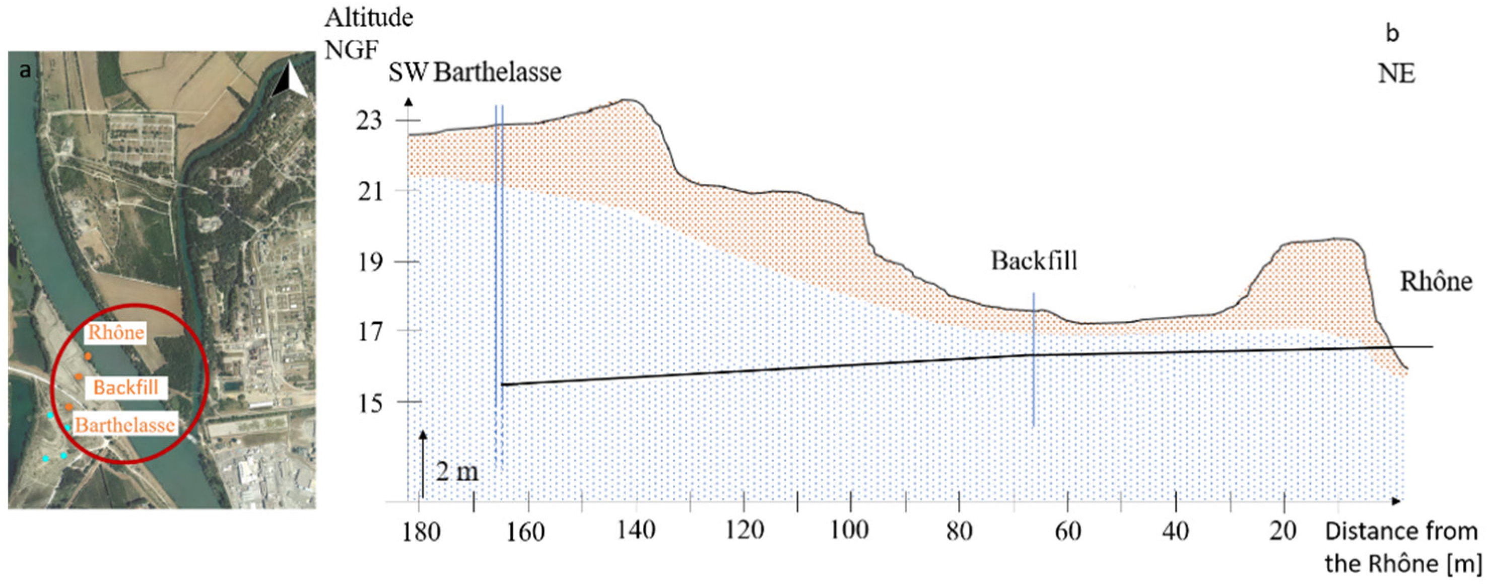
2.1. Study Site

2.1.1. Location and Climate

The Island of Barthelasse is in the southern part of France, near Avignon (Figure 1). The climate is Mediterranean [27,28], characterised usually by dry periods in Winter and Summer. The other feature of rainfall in the Mediterranean environment is its low frequency and intensity. Autumn and the beginning of winter and spring are the two rainy seasons; the equivalent of half of the average annual precipitation can fall in one day during intense rainy episodes, such as stormy Cévennes episodes. The Rhône river valley is marked by the Mistral wind, which is cold, dry and strong, with a mean speed of 50 km/h, and the strongest gust of wind can reach more than 100 km/h. The mistral contributes to the sunshine and drought of this area.

2.1.2. Complex Hydraulic Management

The hydrographic network is complex because of the Rhône river divagation and the river management works made between 1970 and 1973 by the Rhône management company (CNR, Compagnie Nationale du Rhône). In 1970, the hydraulic management of the Rhône resulted in the construction of 18 hydroelectric developments, 330 km of the river corridor, flood protection of 44,000 ha and 120,000 ha of irrigated land [30]. The Island of Barthelasse shape is the result of the works of the CNR over the years. Figure 2 is a time-lapse evolution of the Island of Barthelasse with the creation of second arms of the Rhône River in the west, after the year 1973.

Nowadays, the island is surrounded by two arms, the Villeneuve and Avignon arms on the west and east, respectively. Each one has a regulated flowrate for hydroelectric purposes; most of the flow goes into the Villeneuve part. During the CNR hydraulic management, two small arms were separated from the Rhône River and became backwaters. One of these backwaters (BwB), a few hundred meters wide, divided the Island of Barthelasse into two parts, respectively, the Motte Island in the north and Barthelasse Island in the south. A direct connection between the Rhône River and the BwB occurs on the east when the water level of the river is high enough, usually during the rain events of autumn and spring. The BwB are always fed by water coming from the counter channel on the western part of Barthelasse Island.

Between 1860 and 1880, major works were undertaken on the Rhône over a large part of its downstream course to make it more navigable. In our region, several developments (known as “Girardon” units) were built on the east channel along the right bank of the Avignon arm (in orange in 3). The Girardon structures are rectangular fields installed on the banks of the Rhône in order to stabilise the banks (alluviation) and to favour river navigation [31,32]. These Girardon units were made of both fine sediments (silts and sands) and coarse sediments (pebbles), extracted from the Rhône by dredging [33]. They have modified the hydrological dynamics of the Rhône as well as the sedimentation dynamics.

This study was focused on the east part of the island as shown in black in Figure 3. The Barthelasse pumping field is separated from the Rhône by one of the three Girardon units of the sector and the insubmersible dam at 300 linear meters from the Rhône River.

2.1.3. Geological Context

The aquifer of the Island of Barthelasse is part of the alluvial aquifer of Avignon, composed of alluvial deposits from three rivers: the Rhône, Durance and Ouvèze. The alluvial plain itself is composed of quaternaries “old” and recent alluvium. The first ones are quartzite pebbles coming from the Alps and Cevennes and Massif central. The second composes the main part of the plain with fluvial deposits from the Rhône and Durance rivers. In the Island of Barthelasse, these materials average a thickness of 15 m, increasing from 11 m in the north to 15 m in the south. They are highly heterogeneous due to the old channel of the Rhône River marked locally by molassic rocks. Silts deposits 3 to 4 m thick cover the alluvial material [34].

2.1.4. Hydrogeological Background

In this sector, the static level of the alluvial aquifer is between 14.5 and 16.7 m (msl) (mean sea level). The aquifer is mostly unconfined but may be semi-confined to confined depending on the presence and thickness of silts. The Barthelasse field has four pumping wells and 13 piezometers. The average pumping rate is 5700 m³/day. According to the different pumping tests performed in 1982, the transmissivity is between 0.08 and 0.01 m²·s⁻¹ [35]. The Rhône River contributes to the recharge of the alluvial aquifer differently according to the sector. The flow direction in the Barthelasse Island is from the northeast to the southwest, Figure 3. The main flow direction (Figure 4) is controlled by the CNR management plan made by the dam shown in Figure 1 and the presence of the drain is in the south part of Barthelasse Island. Locally, the groundwater flow directions are also affected by the pumping flow rate dynamics.

The profile studied is as follows: Rhône, Girardon unit, pumping field (Figure 5). Sensors for temperature, groundwater level and electrical conductivity of the water were positioned in the Rhône and two observation wells, in the Girardon unit (Backfill) and in the pumping field (Barthelasse), located, respectively, 67 and 165 m from the Rhône (Figure 5). The parameters were measured at a time step of 15 min. The monitoring was carried out over a period of one and a half years, from 14 October 2018 to 30 January 2020. The gaps were filled by linear interpolation.

The continuous physico-chemical monitoring was supplemented by occasional water samples in order to carry out stable isotope analyses of the water molecule (¹⁸O et ²H) within the Rhône and the two observation wells. Samples were taken fortnightly during this study. During the flood of 21/10/19, a refinement of the water samples took place with an hourly frequency during the peak of the flood and then twice daily at the end of the flood. Automatic samplers, ISCO, were used to collect water from the piezometers and the Rhône. Groundwater was extracted with a 12V PVC submersible sampling pump and stored in brown glass vials closed by a 20-mL bakelite cap for stable isotope analysis with a Picarro L2140-6i spectrometer laser analyser in the laboratory of Avignon University. A control station allowed the pumping to be started 15 min before sampling in order to renew the water in the wells before automatic sampling.

2.2. Theory

2.2.1. Lumped Parameter Models

The analysis of environmental tracer concentration time series via advective-dispersive model fitting is commonly used to determine the origin of water, mixing patterns and age of groundwater. The general approach is to convolve an input time series with a predefined function that represents the distribution of water transit times in the system. These approaches are clustered under the generic term of Lumped Parameter Models (LPMs). These mathematical models offer a simplified and global representation of the flows within the aquifer, taking into account the effects of dispersion and mixing.

The time variation of the output signal is obtained by solving the following equation:

$${\mathrm{C}}_{\mathrm{out}}\left(\mathrm{t}\right)={\int }_{-\infty }^{\mathrm{t}}{\mathrm{C}}_{\mathrm{in}}\left(\mathrm{t}\prime \right){\mathrm{e}}^{-\mathsf{\lambda }\left(\mathrm{t}-\mathrm{t}\prime \right)}\mathrm{g}\left(\mathrm{t}-\mathrm{t}\prime \right)\mathrm{dt}\prime$$

(1)

where:

C_out (t) = the concentration of the tracer at the output

C_in (t’) = the concentration of the tracer at the input at time t’

t = the sample date

t’ = the date on which the water particle entered the system

λ = the radioactive decay constant (for radiogenic tracers)

t−t’ = the age of a water particle

g = the transfer time distribution function

In the present study, the models applied were the dispersion model (DM, Equation (2)) and the exponential mixing model (EMM, Equation (3)) (Kreft and Zuber, 1978; Maloszewski, 2000; Maloszewski and Zuber, 1996):

$${\mathrm{DM}}_{\mathrm{g}\left(\mathrm{t}-\mathrm{t}\prime \right)}=\frac{1}{{\mathsf{\tau }}_{\mathrm{s}}}\frac{1}{\sqrt{4{\mathsf{\pi }\mathrm{D}}_{\mathrm{p}}\frac{\mathrm{t}-\mathrm{t}\text{′}}{{\mathsf{\tau }}_{\mathrm{s}}}}}{\mathrm{e}}^{(-\frac{{\left(1-\frac{\mathrm{t}-\mathrm{t}\prime }{{\mathsf{\tau }}_{\mathrm{s}}}\right)}^2}{4{\mathrm{D}}_{\mathrm{p}}\frac{\mathrm{t}-\mathrm{t}\prime }{{\mathsf{\tau }}_{\mathrm{s}}}})}$$

(2)

$${\mathrm{EMM}}_{\mathrm{g}\left(\mathrm{t}-\mathrm{t}\prime \right)}=\frac{1}{{\mathsf{\tau }}_{\mathrm{s}}}{\mathrm{e}}^{\left(\frac{\mathrm{t}-\mathrm{t}\text{′}}{{\mathsf{\tau }}_{\mathrm{s}}}\right)}$$

(3)

where ${\mathsf{\tau }}_{\mathrm{s}}$ is the mean transit time, D_p is the dispersion parameter = α/x avec α dispersivity and x is the distance between the input and output.

The EMM model proved to be less efficient than the DM model, even though the two models provided consistent results between them. Therefore, in the rest of this study, only the results of the dispersive model will be shown.

2.2.2. Validation

In order to determine the parameters ${\mathsf{\tau }}_{\mathrm{s}}$ and Dp, several optimisation criteria were used:

The RMSE (Equation (4)) is a quantification of the size of the differences between observations and measurements. The RMSE can thus be related to the variance of the model. However, the magnitude of the criterion is not standardised, and is, therefore, dependent on the data used.

$$\mathrm{RMSE}=\sqrt{\frac{{{\displaystyle \sum }}_{\mathrm{i}=1}^{\mathrm{n}}{\left({\mathrm{y}}_{\mathrm{i}}-{\mathrm{y}}_{\mathrm{sim}\mathrm{i}}\right)}^2}{\mathrm{n}}}$$

(4)

where:

i = the number of sample point

y_i = the ith observation value

y_{sim i} = the ith simulation value

n = the total number of sample point

The NSE criterion [36] is a normalised criterion (i.e., calculated in relation to a reference value) constructed from the normalisation of the RMSE criterion. The closer the criterion is to 1, the better the model fits the observed values.

$$\mathrm{NSE}=1-\frac{{{\displaystyle \sum }}_{\mathrm{i}=1}^{\mathrm{n}}{\left({\mathrm{y}}_{\mathrm{i}}-{\mathrm{y}}_{\mathrm{sim}\mathrm{i}}\right)}^2}{{{\displaystyle \sum }}_{\mathrm{i}=1}^{\mathrm{n}}{\left({\mathrm{y}}_{\mathrm{i}}-{\mathrm{y}}_{\mathrm{mean}}\right)}^2}$$

(5)

where:

i = the number of sample point

y_i = the ith observation value

y_{sim i} = the ith simulation value

n = the total number of sample point

y_mean = the mean of the observed values

The KGE criterion [37], evaluates the Euclidean distance between the observed and simulated values. It is derived from the NSE. Since the objective is to reach optimal values, the Euclidean distance must tend towards zero, and the aim is to maximise the KGE. Again, the closer the criterion is to 1, the better the model fits the observed values.

$$\mathrm{KGE}=1-\sqrt{{\left(\mathrm{r}-1\right)}^2+{\left(\propto -1\right)}^2+{\left(\mathsf{\beta }-1\right)}^2}$$

(6)

where:

r = correlation coefficient

β = bias ratio = $\frac{{\mathsf{\mu }}_{\mathrm{sim}}}{{\mathsf{\mu }}_{\mathrm{obs}}}$

α = variability ratio = $\frac{{\mathsf{\sigma }}_{\mathrm{sim}}/{\mathsf{\mu }}_{\mathrm{sim}}}{{\mathsf{\sigma }}_{\mathrm{obs}}/{\mathsf{\mu }}_{\mathrm{obs}}}$

2.2.3. Cross-Correlation Analysis EC

Cross-correlation can be interpreted as the estimation of the correlation between two smoothed and time-shifted time series, i.e., as the application of a parametric transfer function to the time series after the subtraction of their characteristics (Equation (7)).

$$\mathrm{R}\left(\mathsf{\tau }\right)={{\displaystyle \int }}_{-\infty }^{+\infty }\mathrm{x}\left(\mathrm{t}\right)\mathrm{y}\left(\mathrm{t}+\mathsf{\tau }\right)\mathrm{dt}$$

(7)

where:

x(t) and y(t) = two time-dependent functions

τ = the time-shifted variation

These evolutions make it possible to carry out a cross-correlation analysis on the continuous data from the CTDs sensors, and more particularly, on the electrical conductivity data. In our study, we will focus on the cross-correlation analysis between the Rhône signal and the groundwater signal at the two observation wells. The maximum correlation between the two signals will be synonymous with the time shift between the river and the groundwater signal. Before performing the cross-correlation, the signals are normalised by their annual averages to see only the variations of the conductivity during floods. A seasonal filter was applied to remove seasonal variations. The seasonal filter consists of a moving average (unweighted mean of the previous k months), which can be viewed as a low-pass filter.

3. Results

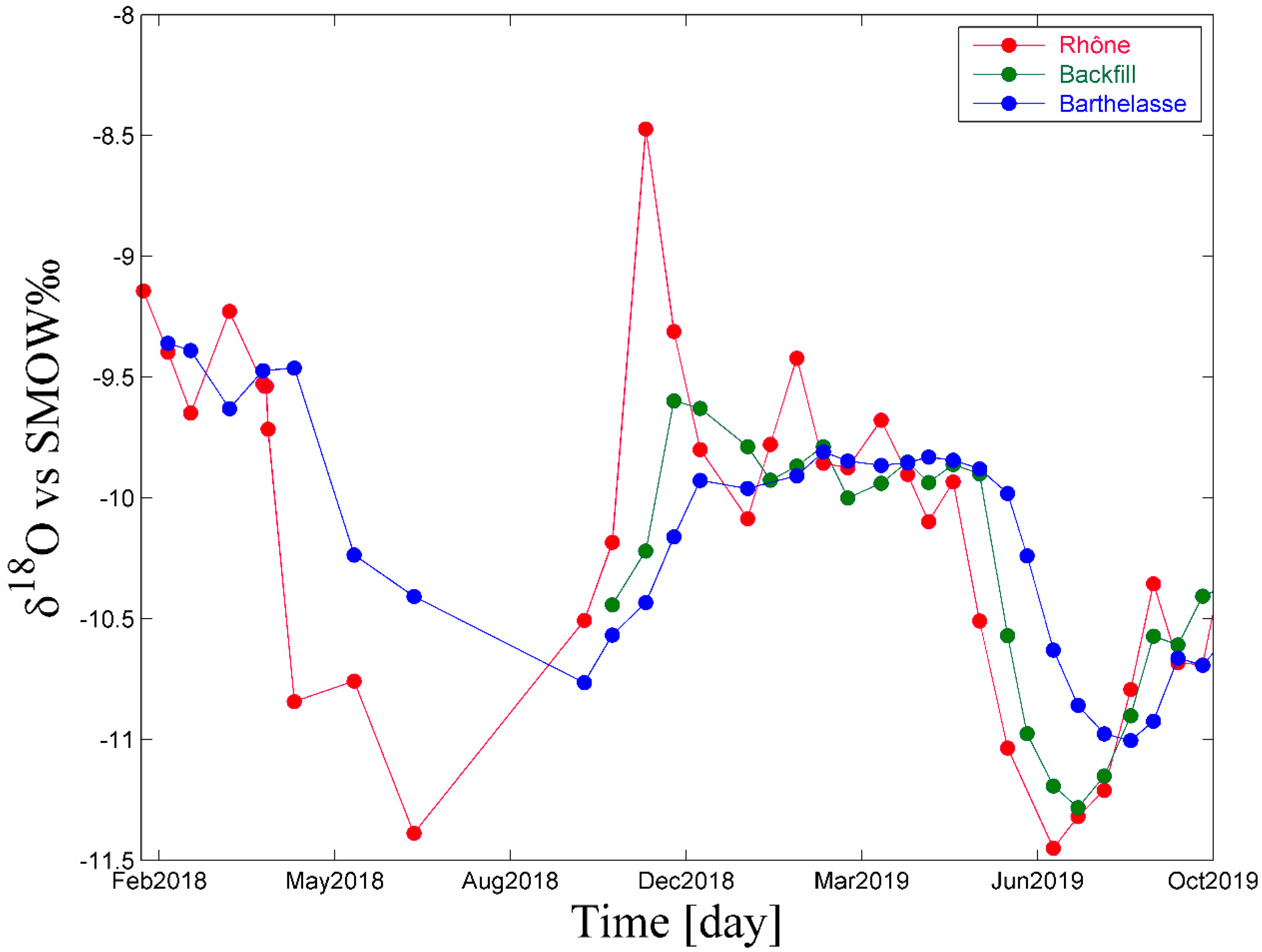
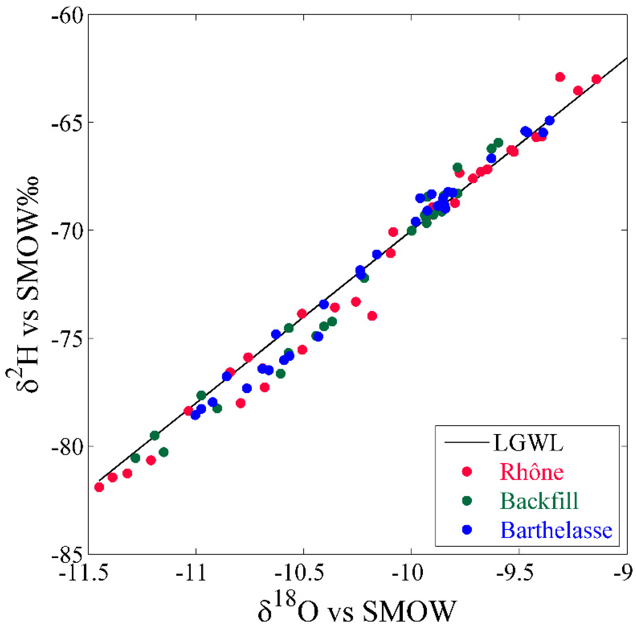
3.1. Annual Scale Monitoring

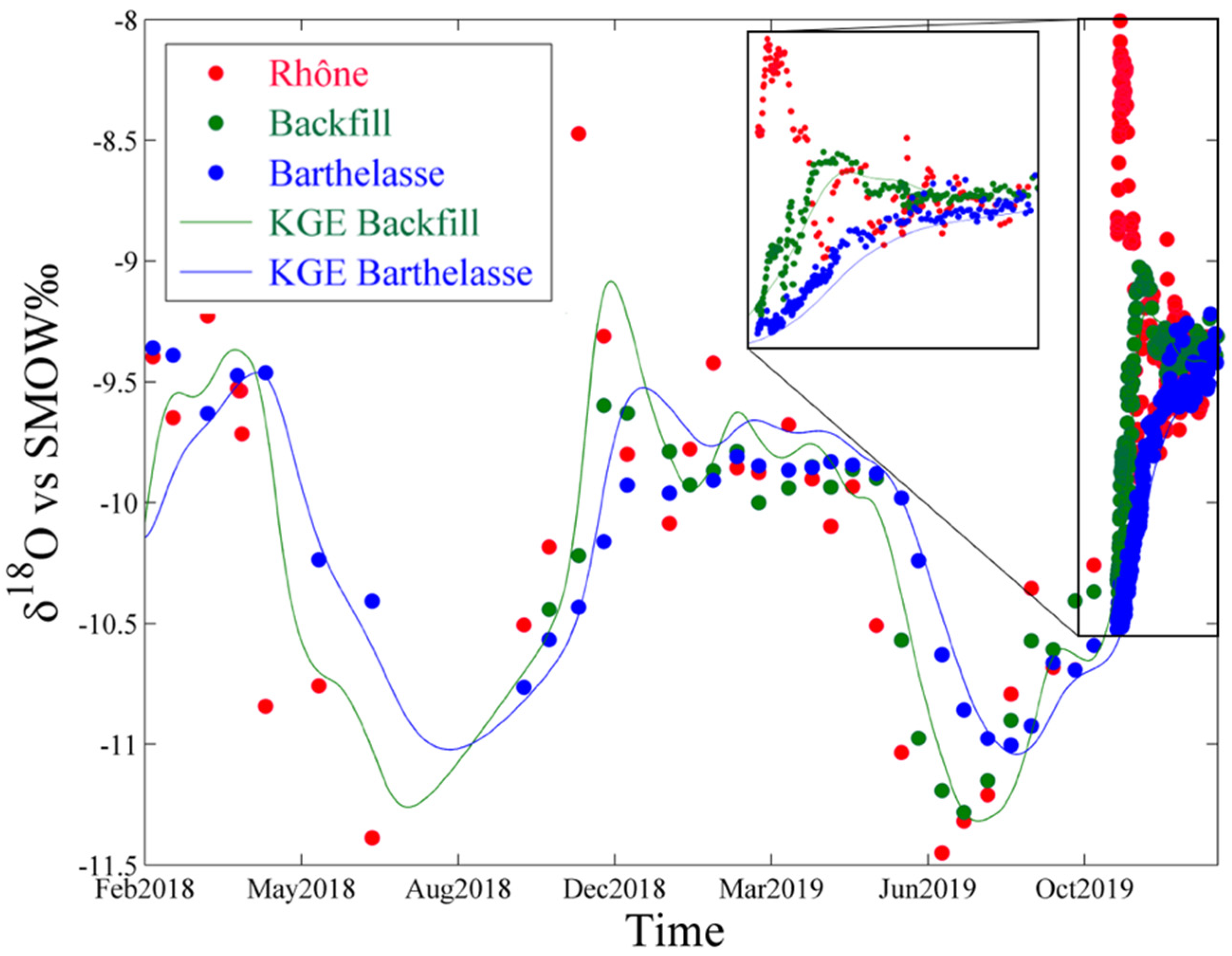
3.1.1. Isotopic Variations over Time

The report study δ¹⁸O et δ²H indicates that the two observation wells and the Rhône are located on the Global Meteoric Water Line (Figure 6) [28]. The Rhône shows a cyclic variation of δ¹⁸O with enriched water in winter and depleted water in summer (Figure 7). The variations within the observation well follow those of the Rhône with the presence of damping and a time lag, which confirms the supply of the Barthelasse pumping field by the Rhône. Except for measurement error, the mean values of δ¹⁸O for each of the monitoring points are similar, with −10.11 for the Rhône, −10.27 for the backfill and −10.17 for the Barthelasse. The standard deviation values demonstrate this damping along the study transect as the value is 0.71 for the Rhône, 0.52 for the backfill and 0.49 for the Barthelasse.

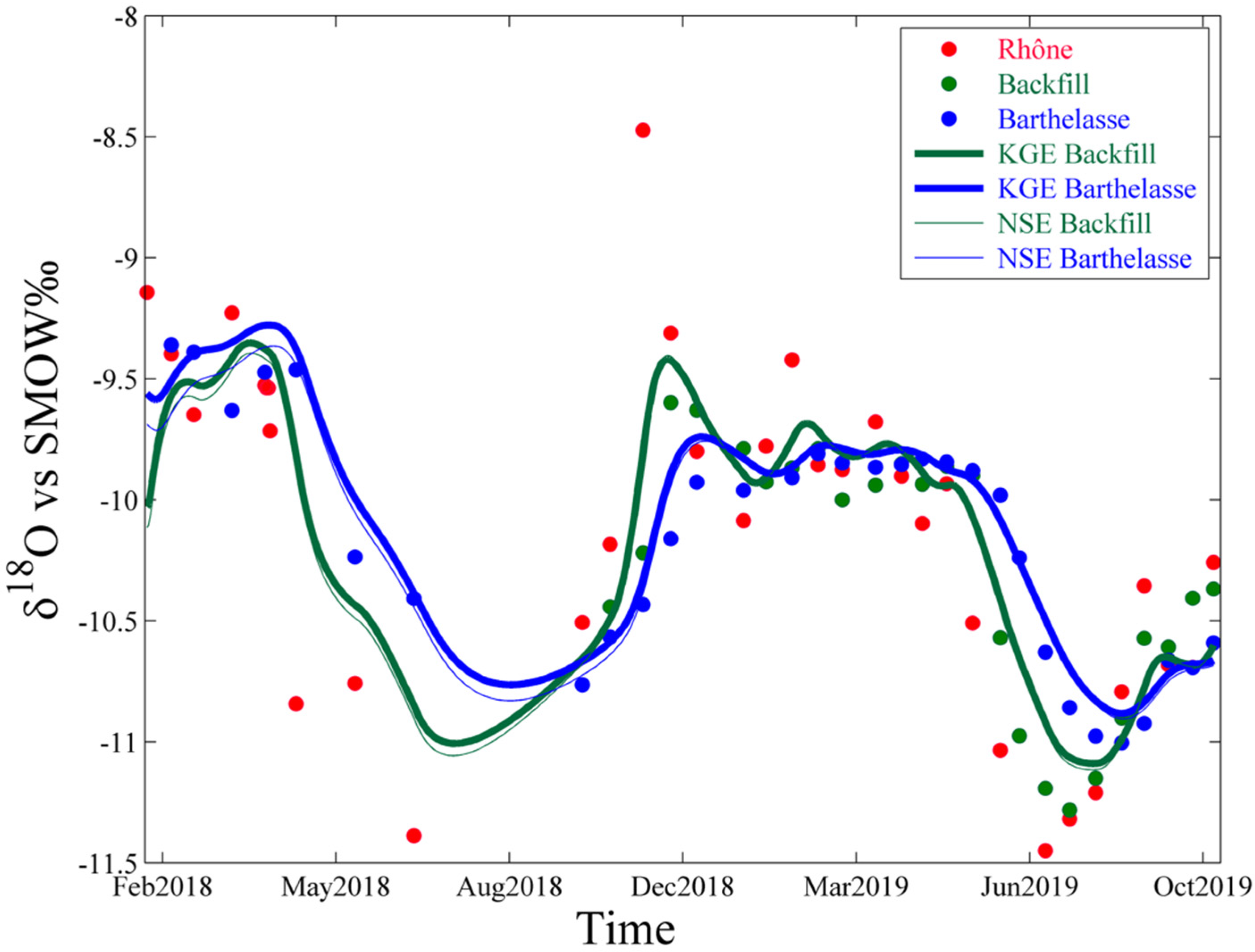
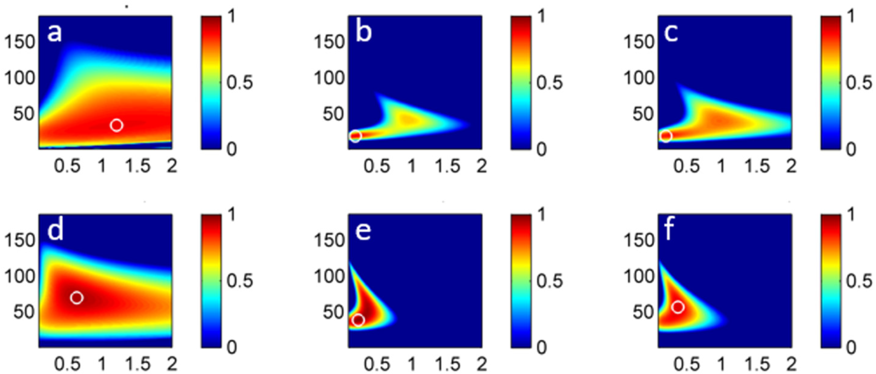
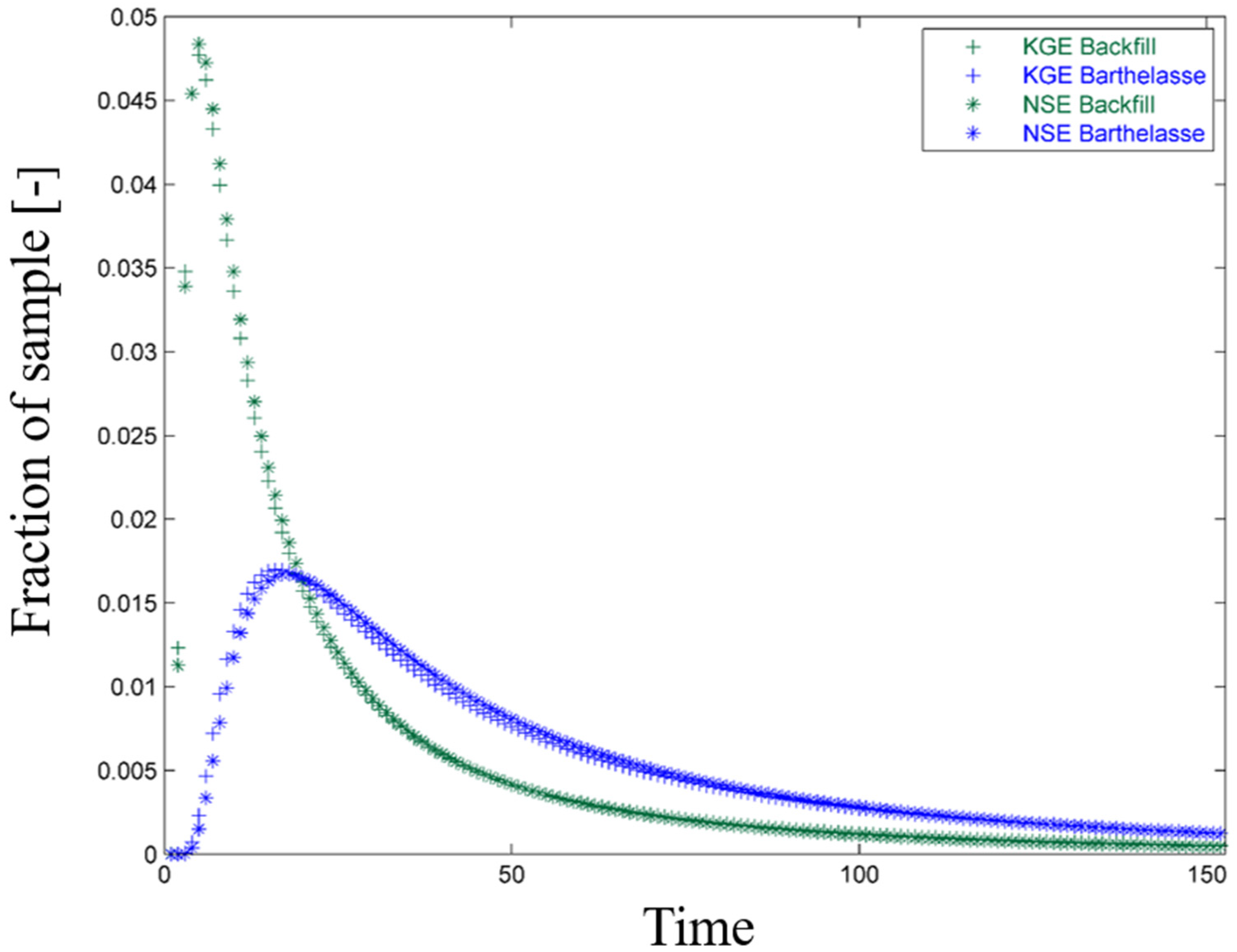
3.1.2. Applications of Lumped Parameters Models

Whether using the KGE or the NSE, the two optimised parameters Dp and τs of the DM model are almost identical, but with slightly higher values for the KGE (

Table 1. Main results of the LPMs applied to the backfill and the pumping field.

		Backfill			Barthelasse
	Dp	τs(j)	Criterion	Dp	τs(j)	Criterion
RMSE	0.99	12	0.18	0.5	61	0.11
KGE	1.4	38	0.94	0.75	74	0.97
NSE	1.21	34	0.88	0.4	70	0.95

, Figure 8). The mean transit time is around 36 days at the backfill (Dp around 1.3) and 72 days at the Barthelasse (Dp around 0.7) (Table 1, Figure 9). The parameters obtained from the RMSE criterion are lower. In all cases, the mean transit times are doubled between the backfill and the Barthelasse, while Dp is twice as low for the Barthelasse as for the backfill. However, the distance between the Rhône and the Barthelasse is not equivalent to twice the distance between the Rhône and the observation well (165 and 67 m, respectively). This confirms the difference in the nature of the sediments between the reservoir and the pumping field.

The reconstruction of the output data from optimisation by KGE and NSE is better for the Barthelasse than for the backfill, where the values tend to be overestimated (Figure 8). However, for the summer 2019 period, the values of δ¹⁸O are overestimated for both observation wells. The values of δ¹⁸O are also overestimated in winter 2018, especially for the backfill. The reconstructions obtained from the RMSE optimisation criterion are of poor quality (not shown here).

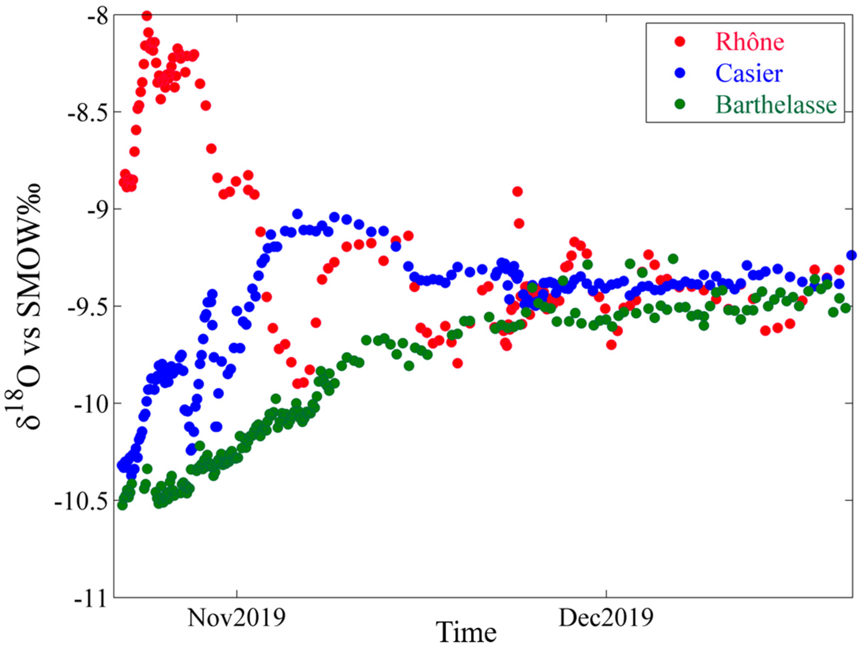
3.2. Event Scale Monitoring

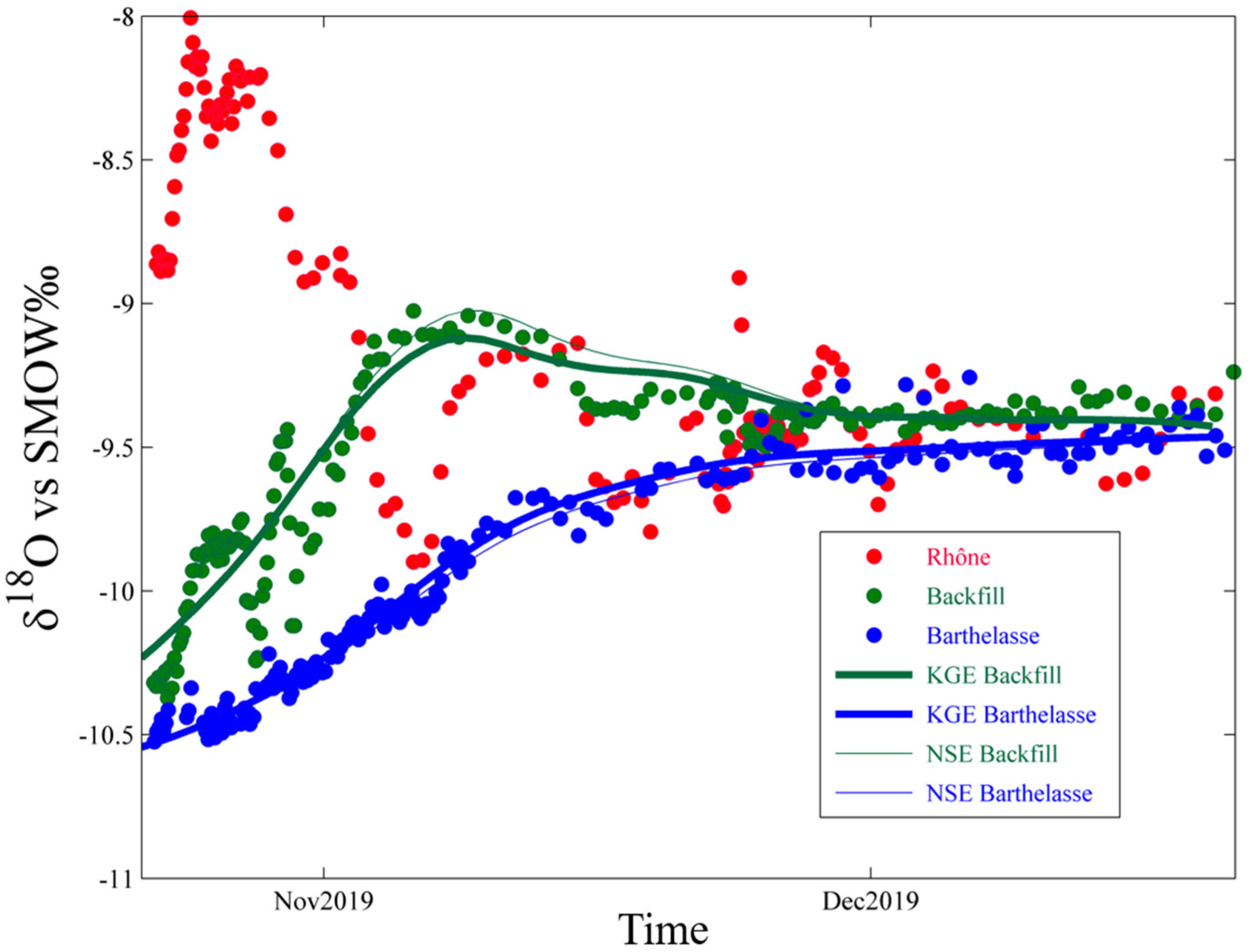
3.2.1. Isotopic Variations over Time

At the end of 2019, following two consecutive floods (21/10/2018 and 24/11/2018), the level of the Rhône increased by 40 cm. This pressurisation of the system can be seen in the Girardon unit with an increase of 26 cm but is hardly visible in the Barthelasse piezometer, given the presence of uninterrupted pumping within the field, which generates water level variations ranging from 20 to 50 cm. However, the isotopic signature of this flood is visible, so it is possible to determine the transfer time between the Rhône and the pumping field using δ¹⁸O. The Rhône shows an enriched isotopic signature following the rainfall of the Cevenol episode, with a maximum of −8.01‰ and a mean value of −9.11‰ (Figure 10). This isotopic enrichment can also be seen in the backfill with a maximum at −9.02‰ and a mean value of −9.55‰. The Barthelasse has the most damped enrichment with an average value of −9.90‰.

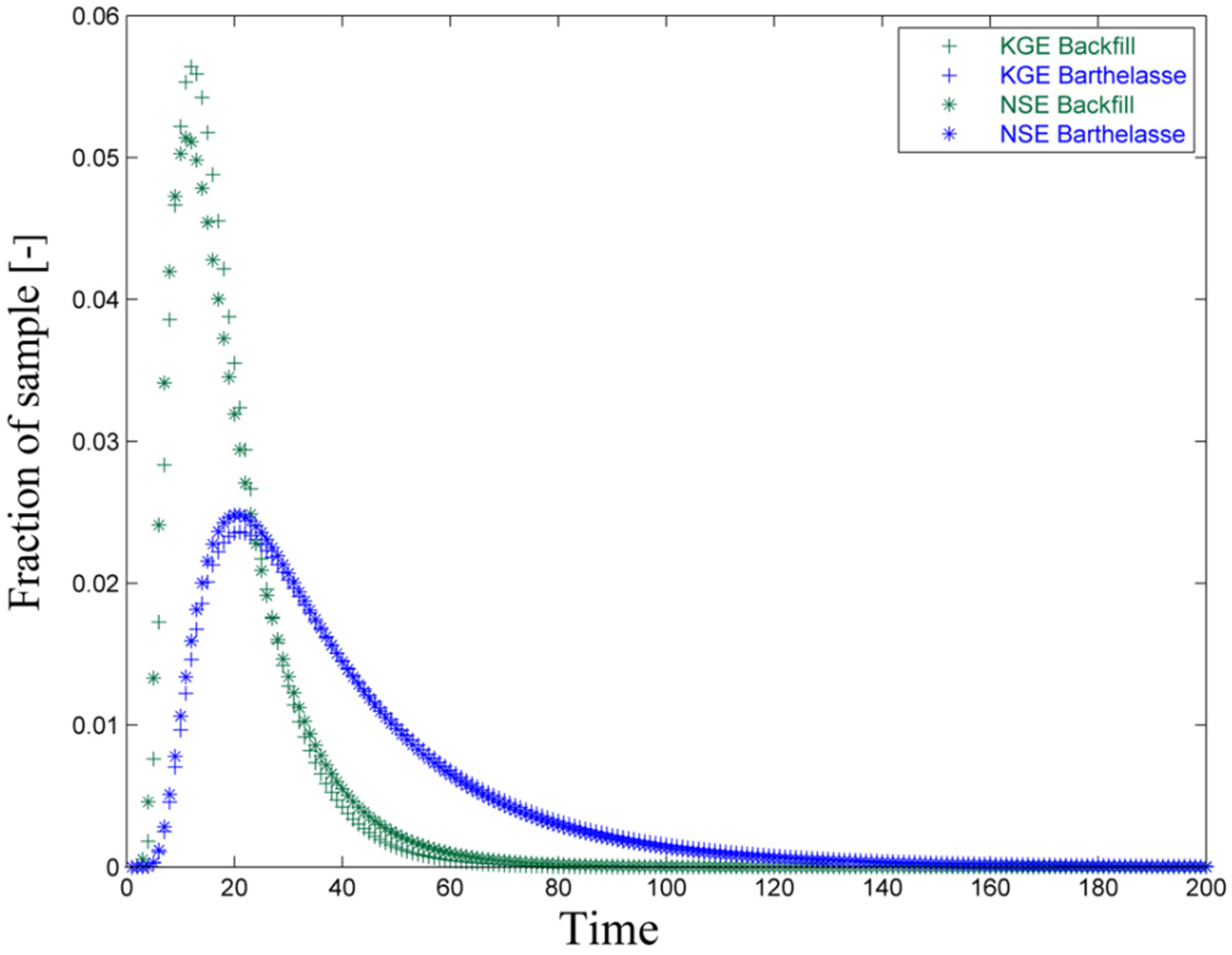
3.2.2. Applications of Lumped Parameters Models

In contrast to the annual data, the two model parameters for the two observation wells are almost identical for each criterion (

Table 2. Main results of the LPMs applied to the backfill and the pumping field.

		Backfill			Barthelasse
	Dp	τs(j)	Criterion	Dp	τs(j)	Criterion
RMSE	0.18	20	0.09	0.23	40	0.06
KGE	0.15	18	0.93	0.25	41	0.99
NSE	0.20	19	0.88	0.24	39	0.97

). The Dp values are close to each other for both observation wells, with low values ranging from 0.15 to a 0.25 maximum. The mean transit time estimated by the flood monitoring are lower than those estimated by the annual model, with the exception of the estimation at the backfill with the RMSE criterion, whose Ts value has increased from 12 to 20 days. However, the mean transit times remain twice higher for Barthelasse than for the backfill.

Within the backfill, the proportion of young water is still important, but the distribution appears to be centred around the value of 12 days, contrary to the distribution resulting from the annual model parameters (Figure 11). For the Barthelasse piezometer, the annual and flood distributions have the same shape, with a more pronounced maximum, indicating an increase in the proportion of young water.

The reconstruction of the isotopic curve for the Barthelasse well is better than for the backfill (Figure 12). Indeed, in the first few days at the backfill, a rapid decrease followed by a rapid increase in the value in δ¹⁸O was visible, but the models failed to reconstruct it correctly.

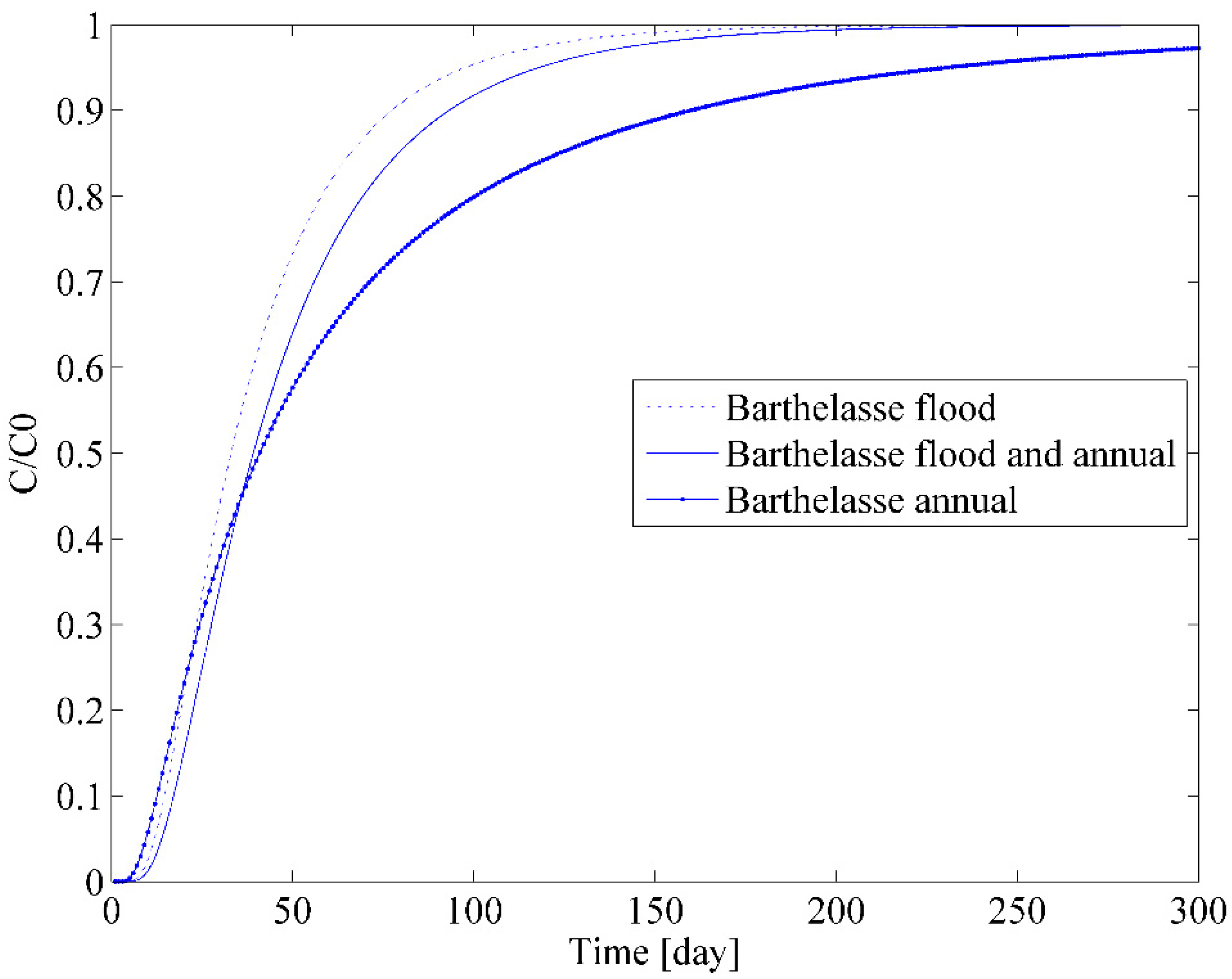
3.3. Combining Annual Scale and Event Scale Monitoring

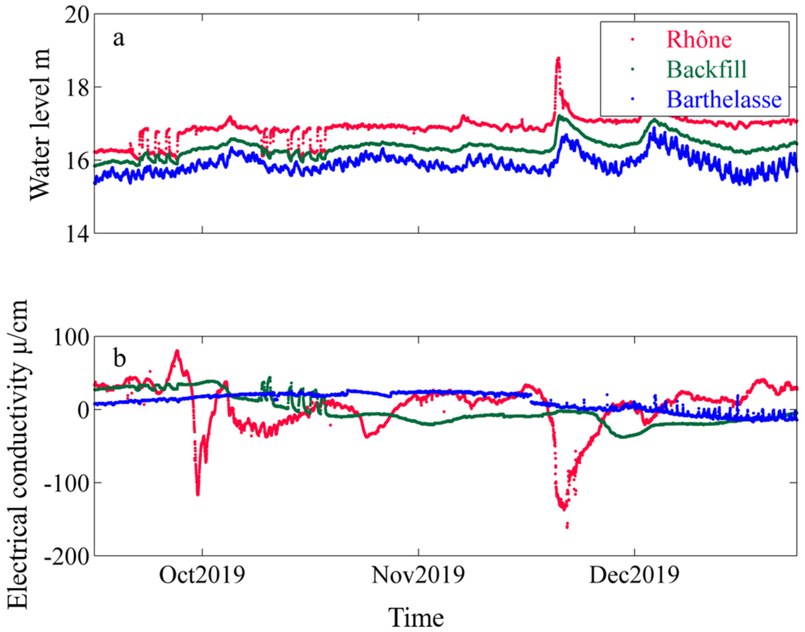
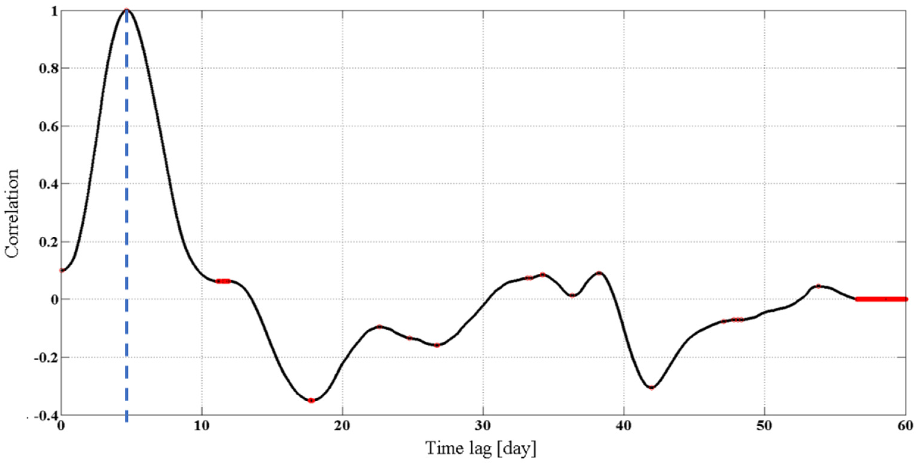
A sensitivity analysis of the parameters was conducted from the results of 142,104 simulations (Figure 13). The estimation of the transport parameters for the annual data shows a high variability according to the parameter Dp for the backfill and a lower variability according to the mean transit time. The results for the Barthelasse also show variability on an annual scale, this time around a lower Dp value (ranging from 0.5 to 1) and a high mean transit time value.

The high-frequency monitoring considerably reduces the variability of the two parameters. The optimised Dp parameter is this time comparable for the two sites with a value of 0.15 and 0.25 for the backfill and Barthelasse, respectively.

The comparison of the maps of Dp/τ_s obtained for the low and high sampling frequencies shows that there is a small area, common to both sets, where the criterion is greater than 0.8. The method consisted in crossing the maps of Dp/τ_s obtained for the low and high sampling frequencies to define new optimal values of the two parameters.

The optimal couple of parameters for the backfill is Dp = 0.20 and τ_s = 20 days and for the Barthelasse Dp = 0.26 and τ_s = 49 days. These couples are close to the values obtained during the study of the flood with a low Dp. The reconstitution of the data in the backfill, by combining the two models, improves the estimation of the values in the summer period and simulates the second flood with more accuracy, although the values remain overestimated for the first winter period (Figure 14). The simulated data for the Barthelasse show a good correlation with the data measured during the study, although the values are overestimated during the winter period and underestimated during the flood period in 2019. However, this reconstruction represents the best compromise.

3.4. EC Analysis

Both EC and temperature fluctuations in the river and groundwater show a seasonal and inverse variation. In summer, the temperature in the river is higher than in the groundwater and vice versa in winter. However, the EC is of interest during flood events. Indeed, flood events will have the effect of reducing the mineralisation of river water and thus produce a clearer diluting input signal to the aquifer. These intense and rapid variations in the river regime propagate into the associated aquifer in which the water will become mineralised as its residence time increases. During the various floods of the Rhône, the groundwater level in the reservoir increases almost instantaneously (Figure 15). Each of the Rhône’s floods is accompanied by a more or less significant decrease in the EC. This decrease in EC is not proportional to the increase in water level, as the floods of the Rhône may have different origins due to its many tributaries. The dilutions of the EC are reflected in the aquifer, within the reservoir, with the presence of a time lag. High-frequency monitoring of the EC can reveal rapid exchanges that are not always visible from an isotopic point of view. This is a possible situation in the reservoir because of the proximity of the observation well to the Rhône, but the analysis could not be conducted at the pumping field because the fluctuation observed is of the order of magnitude of the measurement error (Figure 15).

Concerning the flood of 21–22 October 2019, the EC reached a minimum of 343 µS/cm on 22 October 2019 at 08:15. The cross-correlation analysis between the Rhône and the reservoir was carried out for this event.

The maximum correlation was obtained for a time lag of 7 days between the two data sets (Figure 16). This time lag can be equated to the rapid transfer time between the Rhône and the reservoir. The analysis of the electrical conductivity is relevant in this kind of system, although spatially limited. In this study, the conductivity results in a transfer time of 7 days, which is particularly short compared to the average transfer time obtained by isotope analysis. However, the distribution of transfer times resulting from the isotope data analysis during the flood of 21–22 October 2019 peaks at 8 days for the backfill.

4. Discussion

4.1. Vulnerability of the Pumping Field and Role of the Backfill

The parameters obtained allow the one-dimensional dispersion equation to be solved using the Ogata-Bank solution [38] for each of the Barthelasse wells and to obtain the concentration of a non-reactive pollutant as a function of time in the case of a step injection (Equation (8)).

$$\frac{\mathrm{C}}{{\mathrm{C}}_0}=\frac{1}{2}\left[\mathrm{erfc}\left(\frac{1-\frac{\mathrm{t}}{\mathsf{\tau }}}{2\sqrt{\frac{\mathrm{t}}{\mathsf{\tau }}\frac{\mathrm{D}}{{\mathrm{V}}_{\mathrm{e}}\mathrm{x}}}}\right)+{\mathrm{e}}^{\left(\frac{{\mathrm{zV}}_{\mathrm{e}}}{\mathrm{D}}\right)}\mathrm{erfc}\left(\frac{1+\frac{\mathrm{t}}{\mathsf{\tau }}}{2\sqrt{\frac{\mathrm{t}}{\mathsf{\tau }}\frac{\mathrm{D}}{{\mathrm{V}}_{\mathrm{e}}\mathrm{x}}}}\right)\right]$$

(8)

where C₀ = initial concentration, t = time, τ = mean transit time, D = dispersion coefficient, Ve = flow velocity, x = distance.

The three curves represent the restitution of the pollutant as a function of time in the Barthelasse well for the three solutions: flood scale, annual scale and the combination of the two (Figure 17). The curve corresponding to the flood (blue dot) is particularly steep due to its short average transfer time in connection with its proximity to the Rhône and its low dispersion coefficient. The differences between the curves are not very sensitive for low relative concentrations but become very noticeable when the C/C0 ratio exceeds 0.5. A total of 10% of the pollutant arrives at the Barthelasse well in around 15 days whatever the model used, but for a 90% restitution, the times are 78, 160 and 95 days, for the “flood” model, the “annual” model and the “combined” model, respectively. These results show that we can be fairly confident about the estimate of the minimum warning time in a case of pollution, but strong uncertainties persist on the knowledge of the transfer dynamics of solutes.

As the distance between two observations wells and the Rhône is known along the same flow line, it is possible to calculate the effective water velocity in the aquifer’s saturated zone. The actual velocities were calculated for three transects, Rhône-backfill, Rhône-Barthelasse and backfill-Barthelasse (98 m) with the three model’s analyses (

Table 3. The effective velocities for three transects, Rhône-backfill, Rhône-Barthelasse and backfill-Barthelasse.

Transect		Rhône-Backfill			Rhône-Barthelasse			Backfill- Barthelasse
	Flood	Annual	Both	Flood	Annual	Both	Flood	Annual	Both
Effective Velocity (m/d)	3.72	1.76	3.35	4.02	2.35	3.37	4.26	2.72	3.38

). The average velocity is of the order of 3 m/d, with a high variability according to the models. For the three transects, the highest velocity is always estimated from the “flood” model. The average velocity on the backfill-Barthelasse section is higher than that estimated on the Rhône-backfill section for two out of three models. The average velocity is in the same order when referring to the combined model. From the calculated Dp values, it is possible to estimate the dispersivity on the Rhône-backfill transect and on the Rhône-Barthelasse transect. This gives values of α = 14 m for the Rhône-backfill transect and α = 43 m for the Rhône-Barthelasse transect. The values obtained are consistent with the scale of the system studied. These differences in velocities between the two transects can be explained by the difference in the composition of the environment between the backfill and the Barthelasse pumping field area. The backfill is made up of a mixture of coarse and fine materials reconstituted by the dredging of the river, constituting a heterogeneous environment and probably favourable to the emergence of preferential flows. Nevertheless, the strong variability of the results encourages the need to be cautious about the conclusions concerning the actual role of the Girardon units on the groundwater flow. The depositional conditions of these units and the types of deposits involved must vary greatly according to the sectors along the Rhône so that it is difficult to attribute a definitive and unique role to these banks layouts. The impact of these units must, therefore, be analysed on a case-by-case basis.

4.2. Rhône Dynamics and Impact on Sampling Frequency

The Rhône watershed is made up of three mountain ranges, the Alps, the Cévennes and the Jura. Snowmelt causes high river flows, especially in spring. The Rhône is also impacted in its southern part by the Mediterranean autumn episodes, which are characterised by high intensity and a high amount of rain, causing flash floods. As a result, the Rhône is fed by various tributaries with different hydrological regimes, which gives it a complex hydrological regime [39,40,41]. However, the flow of the Rhône is controlled by numerous dams, and its natural flow is strongly modified by human activities.

This diversity of water origins results in a very marked isotopic cyclicity of the Rhône throughout the year. The isotopic signature is dependent on latitude and altitude, particularly in a contrasting morphology, such as that of the Rhône watershed, and the stable isotopes of the water molecule are, therefore, very relevant in determining the origin of the water. In summer, the isotope content is rather low because the water mainly comes from the upstream basins, in particular, via the snowmelt. In autumn, the water is rather enriched in heavy isotopes due to floods from the Mediterranean basins (Ardèche, Cèze, Gardon).

At the level of Avignon, even if the autumn floods remain limited in extent due to the control by the Sauveterre dam, the hydrological dynamics are illustrated by the strong isotopic variability observed. This reactivity may seem surprising considering the size of the river. The annual and event-based isotope monitoring demonstrate the rapid dynamics of the Rhône and thus the need to adapt the sampling frequency according to the monitoring season in order to be able to highlight the sudden and rapid changes that can occur. Furthermore, the study shows that the final parameters τ and Dp are close to those obtained for the flood, the estimated average transfer time being of the order of 20 days between the Rhône and the backfill, which is close to the fortnightly sampling frequency on an annual scale. However, when we apply these optimal parameters, the simulated values within the backfill are overestimated for the first flood, which can be explained by the high variability of the isotopic signal during the hydrological cycle. This is why sampling on a 15-day scale does not allow us to intercept all the temporal variations of the δ¹⁸O. In the case of a river such as the Rhône, it seems more relevant to monitor an isotopically marked flood event in order to obtain the conservative transport parameters within the aquifer. Furthermore, the isotopic analysis of the annual data showed the presence of a majority of young water in the samples from the reservoir. It can be deduced that the pressurisation of the aquifer system following a flood event favours short transfer times.

4.3. Choice of Optimisation Criteria

The optimisation criteria used to obtain the most relevant media transport parameter values were KGE and NSE. The RMSE did not provide the optimal parameters for the dispersive models. The KGE and NSE are generally of the same order of magnitude. The Nash–Sutcliffe criterion has been one of the most popular criteria used in hydrological modelling over the last decades [42,43,44,45]. Using the standard deviation, it can be interpreted as the comparison of the simulated data against a basic average model. One of the main shortcomings of this criterion is that its optimisation commonly leads to an overestimation of the values simulated by the model. Gupta et al. (2009) showed that variabilities were not properly considered in the NSE criterion. The KGE, on the other hand, considering correlation, bias, the ratio of variances or coefficient of variation, presents a more balanced way of determining the correct estimation of data by a model. The backfill well has a greater variability, which is not correctly considered in the NSE criterion. The data series at the Barthelasse well has greater inertia, as it is less influenced by the presence of the Rhône than the backfill well. As a result, the notion of correlation between the measured and observed data is more important than for the backfill, and the KGE offers the best optimisation solution. In LPM models, the RMSE criterion is the most commonly used. It is recommended to use a standardised criterion instead and to adapt the choice of this criterion (NSE or KGE) to the observed isotopic variability.

5. Conclusions

The joint analysis of isotope monitoring and continuous EC time series has allowed a more refined understanding of the transfer times between the Rhône and the aquifer. One of the main assumptions of the use of LPMs models is the presence of the steady-state of the system. The Rhône in the Avignon branch has had small fluctuations in water level during the hydrological years since its level is regulated upstream by the Sauveterre dam. In our case, we can, therefore, approximate a stationary hydraulic state. On the other hand, the Rhône presents seasonal and event-related isotopic variation as well as variations in EC. This strong ¹⁸O and EC variability in the Rhône is strongly linked to the spatial and temporal distribution of climatic events in this large basin. Isotopic enrichments and strong decreases in EC extending over several days are remarkable in the case of several episodes and are superimposed on a seasonal cyclicity.

The output concentrations of LPMs models depend on the model parameters and the date of the input. In a highly reactive system, such as the Rhône, as an input source, the sampling frequency can have a significant impact on the calibration process of LPMs models. Over the hydrological year, the sampling frequency has an impact on the evaluation of average transfer times. The frequency of 15 days is not relevant for a dynamic river, such as the Rhône, whose hydrogeochemical evolution varies despite the absence of flow variation within the river. It is necessary to adopt a higher frequency in order to take into account the variations that occur during a hydrological cycle. In addition, sampling during a flood at a high frequency also provides valid parameters for reconstructing variations over the hydrological cycle.

In the hydrological and climatic context of the island of Barthelasse, the main pollution factors are anthropogenic. For the Rhône surrounding alluvial aquifer, the industrial pollution is the most important factor because of the exchange between the groundwater and the river water. This study highlighted an average transfer time between the Rhône and the pumping field of 50 days, which enables the pumping field manager to react in the event of pollution in the Rhône and to adapt a pumping strategy to ensure the supply of water to the inhabitants and preserve the quality of the resource.

The presence of Girardon units along the river tends to disrupt exchanges with the water table. In our case, the Girardon unit tends to increase the speed of the water, and therefore, reduce the transfer time of a possible pollutant to the pumping field. With the uncertainty arising from the fact that these Girardon units are probably not always built in the same way and with the same material, it is advisable to study this effect on a case-by-case basis.

References

1. Hérivaux, C.; Maréchal, J.-C. Prise En Compte Des Services Dépendants Des Aquifères Dans Les Démarches d’évaluation Des Services Écosystémiques—Rapport Final; BRGM (Bureau de Recherches géologiques et minières) (Bureau de Recherches géologiques et minières): Orléans, France, 2019. [Google Scholar]
2. Bertrand, G.; Siergieiev, D.; Ala-Aho, P.; Rossi, P.M. Environmental Tracers and Indicators Bringing Together Groundwater, Surface Water and Groundwater-Dependent Ecosystems: Importance of Scale in Choosing Relevant Tools. Environ. Earth Sci. 2014, 72, 813–827. [Google Scholar] [CrossRef]
3. Clark, I.D.; Fritz, P. Environmental Isotopes in Hydrogeology, 1st ed.; CRC Press: Boca Raton, FL, USA, 1997; ISBN 978-1-56670-249-2. [Google Scholar]
4. Das, B.K.; Kakar, Y.P.; Moser, H.; Stichler, W. Deuterium and Oxygen-18 Studies in Groundwater of the Delhi Area, India. J. Hydrol. 1988, 98, 133–146. [Google Scholar] [CrossRef]
5. Herczeg, A.L.; Barnes, C.J.; Macumber, P.G.; Olley, J.M. A Stable Isotope Investigation of Groundwater-Surface Water Interactions at Lake Tyrrell, Victoria, Australia. Chem. Geol. 1992, 96, 19–32. [Google Scholar] [CrossRef]
6. Katz, B.G.; Coplen, T.B.; Bullen, T.D.; Davis, J.H. Use of Chemical and Isotopic Tracers to Characterize the Interactions Between Ground Water and Surface Water in Mantled Karst. Groundwater 1997, 35, 1014–1028. [Google Scholar] [CrossRef]
7. Maloszewski, P. Lumped-Parameter Models as a Tool for Determining the Hydrological Parameters of Some Groundwater Systems Based on Isotope Data; IAHS Publication, IAHS, UKCEH: Wallingford, UK, 2000; Volume 262, pp. 271–276. [Google Scholar]
8. Maloszewski, P.; Külls, C.; Leibundgut, C. Tracers in Hydrology; John Wiley & Sons: Hoboken, NJ, USA, 2011; ISBN 978-1-119-96501-5. [Google Scholar]
9. Stichler, W.; Maloszewski, P.; Bertleff, B.; Watzel, R. Use of Environmental Isotopes to Define the Capture Zone of a Drinking Water Supply Situated near a Dredge Lake. J. Hydrol. 2008, 362, 220. [Google Scholar] [CrossRef]
10. Xu, W.; Su, X.; Dai, Z.; Yang, F.; Zhu, P.; Huang, Y. Multi-Tracer Investigation of River and Groundwater Interactions: A Case Study in Nalenggele River Basin, Northwest China. Hydrogeol. J. 2017, 25, 2015–2029. [Google Scholar] [CrossRef]
11. Kármán, K.; Maloszewski, P.; Deák, J.; Fórizs, I.; Szabó, C. Transit Time Determination for a Riverbank Filtration System Using Oxygen Isotope Data and the Lumped-Parameter Model. Hydrol. Sci. J. 2014, 59, 1109–1116. [Google Scholar] [CrossRef]
12. Maloszewski, P.; Zuber, A. Lumped Parameter Models for the Interpretation of Environmental Tracer Data. Available online: https://www.osti.gov/etdeweb/biblio/439998 (accessed on 27 February 2020).
13. Marçais, J.; Gauvain, A.; Labasque, T.; Abbott, B.W.; Pinay, G.; Aquilina, L.; Chabaux, F.; Viville, D.; de Dreuzy, J.-R. Dating Groundwater with Dissolved Silica and CFC Concentrations in Crystalline Aquifers. Sci. Total Environ. 2018, 636, 260–272. [Google Scholar] [CrossRef] [Green Version]
14. Jafari, T.; Kiem, A.S.; Javadi, S.; Nakamura, T.; Nishida, K. Using Insights from Water Isotopes to Improve Simulation of Surface Water-Groundwater Interactions. Sci. Total Environ. 2021, 798, 149253. [Google Scholar] [CrossRef] [PubMed]
15. Fórizs, I.; Berecz, T.; Molnár, Z.; Süveges, M. Origin of shallow groundwater of Csepel Island (south of Budapest, Hungary, River Danube): Isotopic and chemical approach. Hydrol. Process. 2005, 19, 3299–3312. [Google Scholar] [CrossRef]
16. Anderson, M.P. Heat as a Ground Water Tracer. Groundwater 2005, 43, 951–968. [Google Scholar] [CrossRef] [PubMed]
17. Cirpka, O.A.; Fienen, M.N.; Hofer, M.; Hoehn, E.; Tessarini, A.; Kipfer, R.; Kitanidis, P.K. Analyzing Bank Filtration by Deconvoluting Time Series of Electric Conductivity. Groundwater 2007, 45, 318–328. [Google Scholar] [CrossRef] [PubMed]
18. Hoehn, E. Hydrogeological Issues of Riverbank Filtration—A Review. In Riverbank Filtration: Understanding Contaminant Biogeochemistry and Pathogen Removal; Ray, C., Ed.; NATO Science Series; Springer: Dordrecht, The Netherlands, 2002; pp. 17–41. ISBN 978-94-010-0479-4. [Google Scholar]
19. Sheets, R.A.; Darner, R.A.; Whitteberry, B.L. Lag Times of Bank Filtration at a Well Field, Cincinnati, Ohio, USA. J. Hydrol. 2002, 266, 162–174. [Google Scholar] [CrossRef]
20. Vogt, T.; Hoehn, E.; Schneider, P.; Cirpka, O.A. Investigation of bank filtration in gravel and sand aquifers using time-series analysis. Grundwasser 2009, 14, 179–194. [Google Scholar] [CrossRef] [Green Version]
21. Dudley-Southern, M.; Binley, A. Temporal Responses of Groundwater-Surface Water Exchange to Successive Storm Events. Water Resour. Res. 2015, 51, 1112–1126. [Google Scholar] [CrossRef] [Green Version]
22. González-Pinzón, R.; Ward, A.S.; Hatch, C.E.; Wlostowski, A.N.; Singha, K.; Gooseff, M.N.; Haggerty, R.; Harvey, J.W.; Cirpka, O.A.; Brock, J.T. A Field Comparison of Multiple Techniques to Quantify Groundwater–Surface-Water Interactions. Freshw. Sci. 2015, 34, 139–160. [Google Scholar] [CrossRef] [Green Version]
23. Slater, L.D.; Ntarlagiannis, D.; Day-Lewis, F.D.; Mwakanyamale, K.; Versteeg, R.J.; Ward, A.; Strickland, C.; Johnson, C.D.; Lane, J.W. Use of Electrical Imaging and Distributed Temperature Sensing Methods to Characterize Surface Water–Groundwater Exchange Regulating Uranium Transport at the Hanford 300 Area, Washington. Water Resour. Res. 2010, 46. [Google Scholar] [CrossRef]
24. Unland, N.P.; Cartwright, I.; Andersen, M.S.; Rau, G.C.; Reed, J.; Gilfedder, B.S.; Atkinson, A.P.; Hofmann, H. Investigating the Spatio-Temporal Variability in Groundwater and Surface Water Interactions: A Multi-Technique Approach. Hydrol. Earth Syst. Sci. 2013, 17, 3437–3453. [Google Scholar] [CrossRef] [Green Version]
25. Slimani, R.; Guendouz, A.; Trolard, F.; Moulla, A.S.; Hamdi-Aïssa, B.; Bourrié, G. Identification of Dominant Hydrogeochemical Processes for Groundwaters in the Algerian Sahara Supported by Inverse Modeling of Chemical and Isotopic Data. Hydrol. Earth Syst. Sci. 2017, 21, 1669–1691. [Google Scholar] [CrossRef] [Green Version]
26. AERMC Nappe Alluviale Du Rhône Identification et Protection Des Ressources En Eau Souterraine Majeures Pour l’alimentation En Eau Potable. Volume 3. (Télécharger Le Document). Available online: https://www.eaurmc.fr/jcms/dma_40370/fr/nappe-alluviale-du-rhone-identification-et-protection-des-ressources-en-eau-souterraine-majeures-pour-l-alimentation-en-eau-potable-volume-3 (accessed on 18 August 2021).
27. Nofal, S. Étude Du Fonctionnement Hydrodynamique de La Nappe Alluviale d’Avignon: Impact de l’usage Du Sol Sur Les Mécanismes de Recharge. Ph.D. Thesis, Avignon Unisersité, Avignon, France, 2014. [Google Scholar]
28. Nofal, S.; Travi, Y.; Cognard-Plancq, A.-L.; Marc, V. Impact of Infiltrating Irrigation and Surface Water on a Mediterranean Alluvial Aquifer in France Using Stable Isotopes and Hydrochemistry, in the Context of Urbanization and Climate Change. Hydrogeol. J. 2019, 27, 2211–2229. [Google Scholar] [CrossRef]
29. Poulain, A.; Marc, V.; Gillon, M.; Mayer, A.; Cognard-Plancq, A.-L.; Simler, R.; Babic, M.; Leblanc, M. Enhanced Pumping Test Using Physicochemical Tracers to Determine Surface-Water/Groundwater Interactions in an Alluvial Island Aquifer, River Rhône, France. Hydrogeol. J. 2021. [Google Scholar] [CrossRef]
30. Gentric, J.; Langumier, J. Inondations des villes, inondations des champs: Norme et territoire dans la prévention des inondations sur l’île de la Barthelasse (Avignon). Nat. Sci. Soc. 2009, 17, 257–265. [Google Scholar] [CrossRef]
31. Räpple, B. Patrons de sédimentation et Caractéristiques de la Ripisylve dans les Casiers Girardon du Rhône: Approche Comparative Pour une Analyse des Facteurs de Contrôle et une évaluation des Potentialités écologiques. Ph.D. Thesis, Université de Lyon, Lyon, France, 2018. [Google Scholar]
32. Thorel, M.; Piégay, H.; Barthelemy, C.; Räpple, B.; Gruel, C.-R.; Marmonier, P.; Winiarski, T.; Bedell, J.-P.; Arnaud, F.; Roux, G.; et al. Socio-Environmental Implications of Process-Based Restoration Strategies in Large Rivers: Should We Remove Novel Ecosystems along the Rhône (France)? Reg. Environ. Chang. 2018, 18, 2019–2031. [Google Scholar] [CrossRef]
33. Gaydou, P. Schéma Directeur de Réactivation de la Dynamique Fluviale des Marges du Rhône; CNRS: Lyon, France, 2013; p. 79. [Google Scholar]
34. Abiven, R.; Blavoux, B. Dir. de thèse Etude Hydrochimique Du Fer et Du Manganèse Dans l’aquifère Alluvial d’Avignon (Vaucluse); France. 1986. [Google Scholar]
35. Gourdin, T. Champ de Captage de l’île de La Motte Pompage d’essai, Résultats, Interprétation; France. 1994. [Google Scholar]
36. Nash, J.E.; Sutcliffe, J.V. River Flow Forecasting through Conceptual Models Part I—A Discussion of Principles. J. Hydrol. 1970, 10, 282–290. [Google Scholar] [CrossRef]
37. Gupta, H.V.; Kling, H.; Yilmaz, K.K.; Martinez, G.F. Decomposition of the Mean Squared Error and NSE Performance Criteria: Implications for Improving Hydrological Modelling. J. Hydrol. 2009, 377, 80–91. [Google Scholar] [CrossRef] [Green Version]
38. Ogata, A.; Banks, R.B. A Solution of the Differential Equation of Longitudinal Dispersion in Porous Media: Fluid Movement in Earth Materials; U.S. Government Printing Office: Washington, DC, USA, 1961. [Google Scholar]
39. Etchevers, P.; Golaz, C.; Habets, F. Simulation of the Water Budget and the River Flows of the Rhone Basin from 1981 to 1994. J. Hydrol. 2001, 244, 60–85. [Google Scholar] [CrossRef]
40. Golaz-Cavazzi, C. Modelisation Hydrologique a l’echelle Regionale Appliquee Au Bassin Du Rhone: Comparaison de Deux Modes de Calcul Des Bilans Hydriques de Surface et Etude de Sensibilite a Une Perturbation Des Forcages Climatiques; ENMP: Paris, France, 1999. [Google Scholar]
41. Golaz-Cavazzi, C.; Etchevers, P.; Habets, F.; Ledoux, E.; Noilhan, J. Comparison of Two Hydrological Simulations of the Rhone Basin. Phys. Chem. Earth Part B Hydrol. Ocean. Atmos. 2001, 26, 461–466. [Google Scholar] [CrossRef]
42. Krause, S.; Hannah, D.M.; Fleckenstein, J.H.; Heppell, C.M.; Kaeser, D.; Pickup, R.; Pinay, G.; Robertson, A.L.; Wood, P.J. Inter-Disciplinary Perspectives on Processes in the Hyporheic Zone. Ecohydrology 2011, 4, 481–499. [Google Scholar] [CrossRef] [Green Version]
43. Oudin, L.; Andréassian, V.; Mathevet, T.; Perrin, C.; Michel, C. Dynamic Averaging of Rainfall-Runoff Model Simulations from Complementary Model Parameterizations. Water Resour. Res. 2006, 42. [Google Scholar] [CrossRef]
44. Pushpalatha, R.; Perrin, C.; Moine, N.; Andréassian, V. A Review of Efficiency Criteria Suitable for Evaluating Low-Flow Simulations. J. Hydrol. 2012, 420, 171–182. [Google Scholar] [CrossRef]
45. De Vos, N.J.; Rientjes, T.H.M.; Gupta, H.V. Diagnostic Evaluation of Conceptual Rainfall–Runoff Models Using Temporal Clustering. Hydrol. Process. 2010, 24, 2840–2850. [Google Scholar] [CrossRef]
Figure 1. Location of the study area ([29] modified by Poulain A.).
Water 13 02695 g001
Figure 2. Time-lapse evolution of the Island of Barthelasse. (A) Extract of the first topographic card of the France Kingdom, “Carte Cassini”, from the XVIIIth Century. (B) Extract of the “carte d’Etat major” from 1820 to 1866. (C) Extract of IGN card from 1950. (D) Extract of IGN from 2018.
Water 13 02695 g002
Figure 3. Hydraulic management of the Barthelasse Island ([33] modified by Poulain A.).
Water 13 02695 g003
Figure 4. (a) Map of local groundwater flow directions. (b) Piezometric map of the study site.
Water 13 02695 g004
Figure 5. Monitoring network of physico-chemical parameters using various sensors and the water sampling network set up on Barthelasse Island (a) and cross-section of the Rhône/Girardon unit/Barthelasse transect (b).
Water 13 02695 g005
Figure 6. Relationships between δ2H and δ18O in water samples with the bi-monthly collected from 02/2018 to 11/2019.
Water 13 02695 g006
Figure 7. δ18O evolution in the Rhône, the backfill observation well and the Barthelasse observation well during the year 2018–2019.
Water 13 02695 g007
Figure 8. δ18O evolution in the Rhône, backfill and Barthelasse during the year 2018–2019, and the reconstitution of δ18O data following the DM model calibration (points = field samples, curves = models).
Water 13 02695 g008
Figure 9. Distribution of transit times within the backfill and Barthelasse on an annual scale.
Water 13 02695 g009
Figure 10. δ18O evolution in the Rhône, backfill and Barthelasse during flood monitoring.
Water 13 02695 g010
Figure 11. Distribution of transit times within the backfill and the Barthelasse on a flood scale.
Water 13 02695 g011
Figure 12. δ18O evolution in the Rhône, backfill and Barthelasse during flood monitoring and simulation from dispersive model calibration (points = field samples, curves = models).
Water 13 02695 g012
Figure 13. Map of optimal parameters resulting from the analysis on an annual scale (a) for the backfill, (d) for the Barthelasse; then on a flood scale (b) for the backfill, (e) for the Barthelasse and finally taking into account the two temporal scales (c) for the backfill and (f) for the Barthelasse.
Water 13 02695 g013
Figure 14. Evolution of δ18O in the Rhône, backfill and Barthelasse after combining flood monitoring and annual monitoring.
Water 13 02695 g014
Figure 15. (a)The water level fluctuation in the Rhône River, backfill and Barthelasse as a function of time. (b) Evolution of electrical conductivity after removal of annual and seasonal variations in the Rhône, backfill and Barthelasse as a function of time.
Water 13 02695 g015
Figure 16. Normalised plot of correlation between the EC data series of the Rhône and the backfill as a function of time lag.
Water 13 02695 g016
Figure 17. C/C0 as a function of time in each of the study cases in Barthelasse.
Water 13 02695 g017