Article

Simulation of the Riprap Movement Using the Continuous-Time Random Walking Method

1
College of Hydrology and Water Resources, Hohai University, Nanjing 210098, China
2
Hydraulic Science and Research Institute of Jiangsu Province, Nanjing 210017, China
3
College of Mechanics and Materials, Hohai University, Nanjing 210098, China
*
Authors to whom correspondence should be addressed.
Water 2021, 13(19), 2669; https://doi.org/10.3390/w13192669
Submission received: 17 August 2021 / Revised: 23 September 2021 / Accepted: 24 September 2021 / Published: 27 September 2021
(This article belongs to the Section Hydraulics and Hydrodynamics)

Abstract

:
During the implementation of the riprap project, the underwater migration process of the stones is quite uncertain because of its difficulty to observe. The process of stone transportation is discrete, which makes it unsuitable to be described by a continuous differential equation. Therefore, considering the distribution of stone jumping and waiting, a continuous-time random walk (CTRW) model is established. Based on the actual engineering data, five schemes simulate the one-dimensional motion of riprap underwater and further discuss the spatial distribution and particle size of the riprap. The results show that the CTRW model can effectively predict the riverbed elevation change behavior caused by the riprap project. The suitability of the model for the prediction of riprap movement decreases first and then increases with the increase in the selected width. This indicates that the randomness of the motion of the riprap causes the width of the observation zone to have a significant effect on the overall behavior of riprap movement. When the width is large enough, the influence of the randomness of the motion can be reduced by the average movement behavior within the observation zone. While the observation time of riprap movement is from a short to long time scale, the transport behavior changes from subdiffusion to normal diffusion behavior.

1. Introduction

Riprap is one of the most common materials used to protect the stability of riverbeds and revetments, bridge abutments and pier foundations from scouring [1]. The transport of riprap is similar to the bedload in the broad sense. In the condition of an underlying water surface, these methods used for riverbanks are no longer applicable [2]. The stability evaluation of riprap adopts Monte Carlo simulation, inertia analysis, the Faroson blue point estimation method and others to calculate the riprap under the flow conditions [3,4]. Numerical simulation methods are usually used to simulate the changes in water flow, wind, waves and riverbed morphology caused by the implementation of stone dumping projects. The existing software is generally used for two-dimensional or three-dimensional simulation, and PFC software is commonly used [5,6], namely River2D [7,8], or the discrete element method is used to simulate the conditions and hydrodynamic methods to establish aggregation models, such as the DEM-SHP model [9], DEM-CFD model [10] and CFD-CSM model [11]. Existing research focuses on the impact of stone dumping on the mass and the migration status of the stone. The complex process of riprap transport underwater can be approximated as the transport process of bedload in the river [12], and the bedload transport model is often used to study the riprap movement. Therefore, the actual demand of river management and development has promoted the development of sediment discipline, and the development of the related disciplines has repaid the progress of river management and development of engineering practices. The important indicator of the development of particle flow is the improvement of the basic theoretical research level of river sediment. The study of particle movement in rivers originated from geomorphology and gradually evolved into a branch of hydraulics. Therefore, the traditional theory retains the traces of geomorphology to a certain extent. In addition, the traditional theory also draws heavily on the research results of fluid mechanics. However, according to the existing research results, it was found that the movement of sediment and riprap particles is a complex process that is cross-scale, highly random and coupled with multiple physical processes [13]. Traditional research methods cannot accurately describe the motion characteristics of the complex process of riprap and sediment movement and its physical mechanism. Considering the above problems, new methods to study the movement of particles such as riprap are needed. The probability statistical method theory based on the particle velocity distribution function and its evolution equation can not only reflect the individuality of particle movement but also reflect the common characteristics of particle movement [14]. Because of its cross-scale research advantages, it reflects the probability change process of particles appearing in velocity space and geometric space, as well as the extremely strong coupling ability of the motion characteristics of individual particles and the statistical characteristics of particle clusters. Recently, stochastic dynamics theory has been widely used in the field of gas molecular motion and particle flow [15,16].
The most basic stochastic transport process in science and engineering is the diffusion process. The classic model of the diffusion process is Brownian motion, which has been widely used in the scientific fields of physics, chemistry, biology, finance and others [17,18]. However, in recent decades, with the improvement of the level of research, more studies are concerned with systems with small scales and complicated conditions. These systems present features that deviate from Brownian motion and result from non-standard statistical physics. Therefore, they cannot be simulated well using the model with Brownian motion and standard statistical distributions [19,20]. All these non-Brownian diffusion processes are collectively referred to as “anomalous diffusion”. Due to the heterogeneity of the riverbed environment, the transport of riprap particles often deviates from conventional statistical physical results and exhibits anomalous transport. The application of random walk and random process theory is a novel and feasible research idea. The most important feature of the probability statistical theory of particle flow is the ability to reconstruct the missing links of microscopic motion characteristics and macroscopic statistical laws.
The riprap movement in the riverbed is similar to bedload sediment, which is an inherently stochastic process. Since Einstein proposed a statistical description of sediment transport, he modeled the sediment transport as a series of alternating step lengths and resting periods [10,21]. The probabilistic framework to characterize particle transport attracted substantial attention from scientists in the past two decades, especially the CTRW model [19,22,23,24]. The CTRW model has been successfully applied to predict the time-dependent kinetics of tracers in strongly inhomogeneous media and constant velocity experiments [25,26,27,28].
The movement of the riprap is controlled by the two aspects of necessity and chance [29]. On one hand, for certain riprap particles, the movement is inevitably affected by the condition of the bottom flow rate, which is in accordance with the laws of mechanics. On the other hand, the particle size, the bottom flow rate, the position of the particles on the bed surface and the structural components of the riverbed are all random variables, and their changes conform to the laws of probability theory. In the operation of the riprap project, it is difficult to accurately capture and predict the difference between the transport behavior in different environments and the transformation of the transport process at different scales. Many parameters of the traditional model use empirical formulas or parameters that make them impossible to be directly applied in some specific engineering projects. The actual observations and theoretical calculations often have great deviations. Therefore, it is a practical and feasible direction to use statistics to study the transport of the riprap. The statistics of macroscopic data dismantle the deterministic nature of the transport properties of riprap in random behavior. The statistical results have made great progress under the rapid development of computer theory in recent years. In addition to the increase in computing speed, the statistical method has become one of the main research methods in different research directions through the big data analysis of macro data and the development of artificial intelligence. This study uses a combination of stochastic theory and engineering practice to determine the appropriate statistical distribution, establish a mechanical model for analyzing and simulating the anomalous transport of riprap in the river and quantify the relationship between the model parameters and the internal structure of the riverbed.
The random walking model is the most intuitive model to study the particle diffusion problem by using various statistical methods. It mainly analyzes the statistical law of the anomalous diffusion process and builds a random walking model by means of unconventional statistical methods. In the study of statistical methods for anomalous diffusion, the Lévy distribution is used the most and has been applied successfully to the analysis of anomalous diffusion phenomena in turbulent, aquifer, biological fluid, semiconductor and other media [30]. Extended Gaussian distribution in porous media with a fractal structure demonstrates its advantages in the anomalous diffusion process. Mittag-Leffler distribution has also achieved breakthrough results in anomalous diffusion and signal processing and other fields. The theory of random walking was first proposed by Einstein [29] when he studied molecular motion in fluids. Two fixed variables, such as fixed waiting time and a certain jump step, were proposed to study the Brownian motion behavior of equilibrium fluids. The random walking framework treats the particles as tracers, which will experience two states in the movement (i.e., rest and jump). The jump step is the distance of a single jump, and the waiting time is the elapsed time between two successive jumps. In the original theory, the behavior of random walking did not consider the distribution of jumps and waits but only fixed steps and time as considerations. On this basis, Montroll and Weiss [31] established the continuous-time random walking method (CTRW). In a CTRW framework, a successful walk is decomposed into two parts: a random spatial jump interval and the waiting time between two successful jumps. The distributions of the two parts are dominated by their respective probability density distributions. Scher and Montroll [32] first developed the CTRW model with a long-tailed distribution of waiting times to describe the motion of charged particles in amorphous semiconductors.
In this study, the long-tail waiting time and jump step distribution are used to simulate the anomalous transport behavior of the riprap movement in the river, and the field observation data further validated the effectiveness of the CTRW model in predicting the transport of riprap. We also discuss the spatial distribution of riprap particles with different hydraulic conditions and different particle sizes.

2. Materials and Methods

2.1. Random Walk Theory

The continuous-time random walking theory (CTRW) extends the assumption of a fixed step size and fixed waiting time to the jump step size and a waiting time dominated by probability density distribution on the basis of the random walking theory. In the continuous-time random walking theory, the particle jumping process is composed of the space jumping distance and the waiting time between two successful jumps. The two parameters are determined by the common joint probability density distribution. In actual research, it is found that the jumping step length and waiting time are often irrelevant. This assumption that the jump distance and the stay time are independent is adopted in this study. Then, the jump step distance and waiting time are determined by their own respective distribution densities. In the study, λ ( x ) ,   ω ( t ) are used to denote the probability density functions of the jump step and the waiting time, respectively. The generalized main equations of the CTRW process are obtained by the joint probability density function as follows [30]:
η ( x , t ) = + d x 0 t η ( x , t ) ψ ( x x , t t ) + δ ( t ) P 0 ( x )
where η ( x , t ) is the probability density function for a tracer to just arrive at position x at time t, the initial distribution of particles is P 0 ( x ) and ψ ( x , t ) represents the joint probability density function of the jump step and waiting time.
The probability density function P ( x , t ) of the particle satisfies the following equation:
P ( x , t ) = 0 t η ( x , t t ) Ψ ( t ) d t
where Ψ ( t ) = 1 0 t ω ( t ) d t is the survival probability, indicating the probability that the particles will never move.
By substituting the generalized main Equation (1) into Equation (2), the probability density equation of continuous-time random walking is finally obtained:
P ( x , t ) = + d x 0 t ψ ( x x , t t ) P ( x , t ) d t + P 0 ( x ) ψ ( t )
In the CTRW framework, both space and time are defined as continuous variables, so Equation (3) can consider the equations satisfied in the phase space. Then, a Fourier-Laplace transformation can be applied to Equation (3):
P ˜ ^ ( k , u ) = 1 ω ˜ ( u ) u · P ^ 0 ( k ) 1 ψ ˜ ^ ( k , u )
Equation (4) in the Fourier-Laplace domain is called the Montroll–Weiss equation. In this equation, the probability density distribution properties of the jump step and waiting time can distinguish different transmission operations as the probability of the jump step. When the second-order moment of the distribution diverges and the first-order moment of the probability distribution of the waiting time converges, the transport operation is defined as super-diffusion transport. When the second-order moment of the probability distribution of the jump step converges and the first-order moment of the probability distribution of the waiting time diverges, the operation defines this as diffusion transport. Both are divergent with both the super-diffusion transport operation and this diffusion transport operation, both of which converge to the normal transport state.

2.2. Monte Carlo Modelling for the Riprap Movement

The Monte Carlo method, also known as the stochastic simulation method, is widely used in the context of the greatly improved computing power of today’s electronic computers [33]. This method is based on statistical theory and uses repeated random sampling methods to obtain the numerical characteristics of statistics. When the number of repetitions is sufficient, the numerical solution obtained by the Monte Carlo method can infinitely converge to the real solution. Due to the complexity of the distribution used in this study, Equation (4) in the Fourier-Laplace domain has great difficulty in converting to the time domain. Here, we use the Monte Carlo method to obtain its numerical results. At the same time, this method has great advantages in tracking the trajectory of particles and analyzing the anomalous movement of particles.
The classic advection–diffusion equation (ADE) characterizes the law of fluid mass transport. By solving the ADE, the distribution of particles under the central limit theorem can be obtained. However, in actual observations, it has been found that the central limit theorem will be broken in many cases. For example, the heterogeneity of the aquifer and the non-uniformity of the riverbed structure will cause the equations that conform to the central limit theorem to fail to accurately describe the actual transport behavior. This type of transport that breaks the central limit theorem is called “anomalous transport”. The continuous-time random walking theory describes the “anomalous transport” behavior by defining jump steps and wait times for more of a “wide” probability density distribution. When the probability density distribution returns to satisfy the central limit theorem, the jump step distribution is normal distribution, the waiting time distribution is exponential, Equation (4) will return to the normal form of the advection–diffusion equation. In this study, in order to reflect the “anomalous transport” behavior of the riprap caused by the heterogeneity of the riverbed’s structure, the α stable distribution is used as the jump step distribution, and the Mittag-Leffler distribution is used as the waiting time distribution.
In this study, we divided the motion of the riprap into the direction of flow and perpendicular to the direction of flow and used independent and identically distributed random numbers to simulate the movement process of the whole riprap process.
The waiting time of the exercise process is determined by the following formula:
t n + 1 = t n + τ β t 0 = 0
The displacement in the direction of the water flow is composed of the displacement caused by the collision of the particles and the displacement caused by carrying the water flow, which is determined by the following formula:
x n + 1 l = x n l + ξ α 1 + v · ( t n + 1 t n ) x 0 l = 0
The displacement perpendicular to the direction of the water flow is only caused by the mutual collision of the particles, which is determined by the following formula:
x n + 1 r = x n r + ξ α 2 x 0 r = 0
where τ β is a random number that satisfies the Mittag-Leffler distribution and ξ α 1 and ξ α 2 are random numbers that satisfy the α stable distribution. Random number generation in the study was generated by the following formula.
Among them, the α stable distribution random number that meets the jump step is generated using Equation (8):
ξ α = γ x ( I n ( u 1 ) cos θ cos ( ( 1 α ) θ ) ) 1 1 / α sin ( α θ ) cos θ
Random numbers satisfying the Mittag-Leffler distribution are generated using Equation (9):
τ β = γ t I n ( u 1 ) ( sin ( β π ) tan ( u 2 β π ) cos ( β π ) ) 1 / β
where u 1 , u 2 ( 0 , 1 ) are uniformly distributed random numbers and γ x , γ t is the scale factor generated by the random numbers.
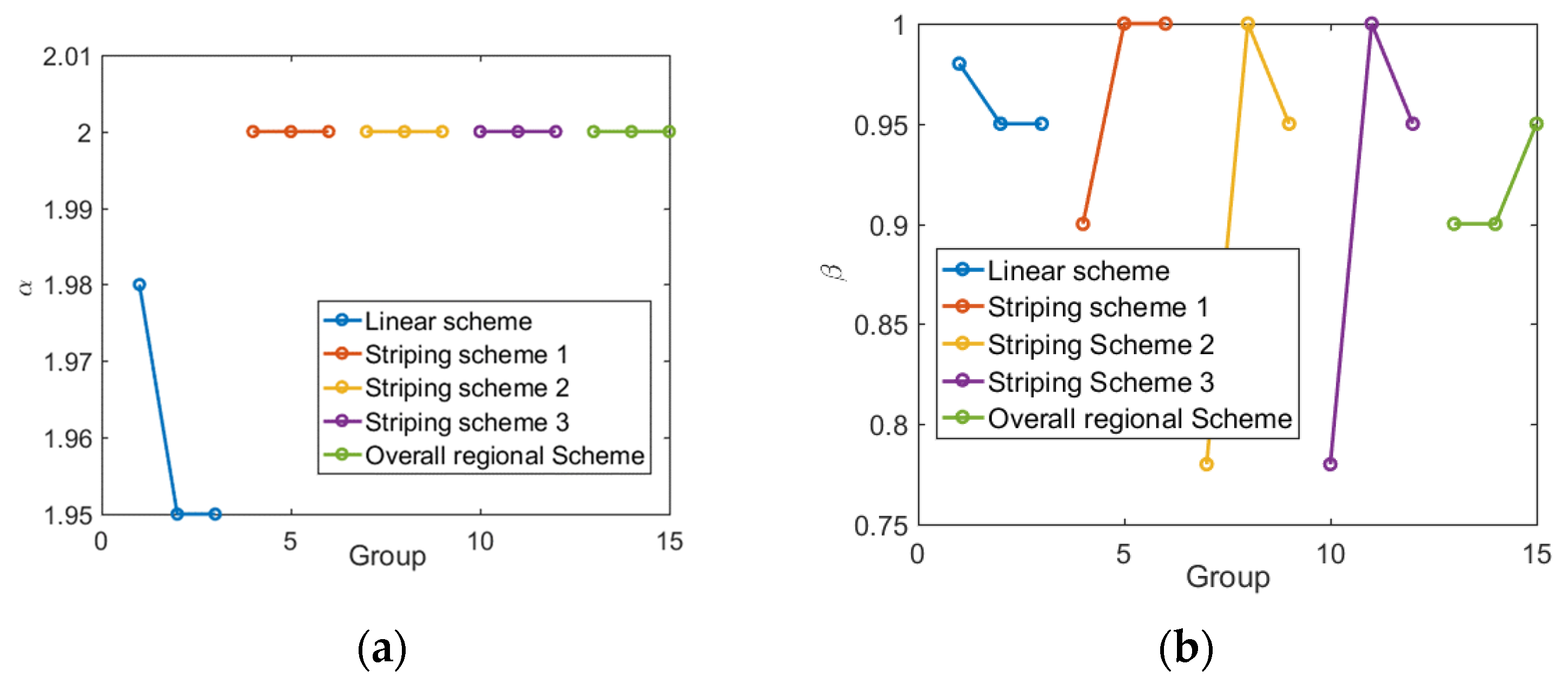
In the actual simulation, we used Equations (5)–(7) as the calculation of the movement displacement of the riprap along the flow direction and perpendicular to the flow direction. The random numbers of the waiting time and jumping step in the formula were determined by Equations (8) and (9), respectively. When the parameter α was larger, the distribution of the jump step was more concentrated (otherwise, it was more dispersed), and when α = 2.0, the distribution of the jump step returned to the normal distribution. When the parameter β was larger, the waiting time distribution had the greater decay rate. When β = 1.0, the waiting time distribution returned to the exponential distribution. A more dispersed jump step distribution means that the riprap particles have a greater probability of performing long-distance movement in a short time. While the waiting time distribution decay is slower, the probability of the riprap particles staying in the riverbed is greater. In the following research, we will analyze the transport behavior of the riprap in the riverbed based on this property. In the simulation, three parameters need to be determined: α is the parameter of α stable distribution which controls the strength of the super-diffusion, β is the parameter of the Mittag-Leffler distribution which controls the strength of subdiffusion, and v is the mean velocity of all the riprap particles. The boundary condition upstream is a Dirichlet condition, and the boundary condition downstream is natural.

2.3. Field Investigation of Riprap Projects

The old sea dam node comprehensive improvement project in Zhangjiagang, which is located in the Chengtong section of the lower Yangtze River, was selected as the study area. The channel is 2 km wide, and the water level during the simulation period was from −0.3 m to about 2.7 m (all based on the 1985 Chinese national elevation datum). The study area belongs to the tidal river section. Under the dual effects of runoff and tide, the flow velocity changes periodically (0.3–1.6 m/s). The river regime changes drastically, with siltation on the left bank and scouring on the right bank. The elevation of the riverbed presented is from −16 to about −5 m on the left bank and from −36 to about −50 m on the right bank. There are many thorough scour pits from −30 m to about −50 m, and the monthly variation of the scouring and silting thickness in individual locations is more than 10 m [34]. Figure 1 shows the specific locations of the study area.
The stone dumping methods used in river improvement work are divided into two types: stone dumping on the outer slope of the embankment and stone dumping in the deep-water area out in front of the wharf. The anti-collapsing layer (particle size: 0.16~0.4 m) is first thrown along the slope foot and then thrown along the bank slope. There are large stones (particle size: 0.5 m~0.65 m), the designed riprap width is 40~120 m, and the total riprap volume reaches 2.442 million m2 [35].
For further verification of the applicability and spatial suitability of the continuous-time random walking model in the transport of the riprap, we used the biharmonic spline interpolation method to interpolate the data collected in the field test at intervals of 0.05 m and performed simulation analysis. The data acquisition used the R2SONIC 2024 multibeam bathymetry system, which uses multiple arrays and wide-angle transmission and reception and has the advantages of measurement accuracy and wide coverage. The horizontal accuracy was ±0.03 m, the sounding accuracy was ±0.05 m, and the range resolution was 0.0125 m. Here, we conducted on-site monitoring of the changes in riverbed elevation at different periods after the riprap projects. Six elevation datasets were obtained on 22 May 2015, 21 July 2015, 18 December 2015, 11 March 2016, 22 May 2016 and 4 July 2016. Among them, there was no riprap project after July 2015. Therefore, the change in riverbed elevation after July 2015 was mainly caused by the transport of the riprap in the river. In order to accurately predict the riprap movement and apply the data to the continuous-time random walking model, we first needed to understand the initial riverbed state before the simulation time and analyze the riverbed elevation data obtained by examining each time. We selected the riverbed elevation data captured for the second instance (21 July 2015) as the initial elevation state of the riverbed. The data measured on 22 May 2015 was not used as the initial state because the difference was too obvious compared with the subsequent data and the elevation distribution for 22 May 2015 was very uneven. This was caused relatively from the fact that the riprap project was still in progress during this period, which had a great impact on the river elevation. Using it as the initial data during the simulation would cause the simulation results to distort and not truly reflect the impact state of the riprap project after the implementation of the riprap project. In order to accurately characterize the degree of change of the riverbed at different times, several sets of data with uniform changes were selected for analysis, namely 20150721, 20151218, 20160311 and 20160522. Due to the difference in the amount of data collected at each time, the riverbed elevation of the uncollected part was subjected to a second interpolation calculation to keep the amount of data consistent. By analyzing the topographic characteristics of the study area and the construction conditions of the rubble project, it was found that the riverbed had a large elevation drop in the direction of the vertical river, and the riprap project was also implemented perpendicular to the riverbank. The change of two characteristics in the vertical riverbank direction was consistent, while the characteristics in each cross section were similar. Therefore, the problem of stone migration in the direction of the vertical riverbank could be generalized into a one-dimensional model for simulation. The simulation path selected by the linear scheme was the most representative feature location in the range, and the location was slightly different in different sessions. For details, refer to the location represented by the linear scheme in the riverbed topography distribution map of different simulation periods in Figure 1.
In order to verify the spatial suitability and spatial scale of continuous-time random walking in the simulation of the riprap movement, the region selection in the study shown in Figure 1 adopted a linear scheme, strip scheme and regional overall scheme. In the linear scheme, the calculated path of the riverbed elevation was the path shown in the “linear scheme”. In each strip scheme, the calculation range was the area between the two straight lines indicated by the double arrow in Figure 1 (different colors represent different stripping schemes), and the overall scheme was calculated in the entire space. The elevation of the calculation path of the stripping scheme, and the overall scheme was the mean value of the elevation along the stripping width direction (calculating the average height along the X axis).

3. Results

3.1. Numerical Simulation Based on the Field Investigation Varied by Different Widths of Observation Strips

The simulation transport results for five different schemes are shown in Figure 2, and the best fitted parameters are listed in Table 1. In the simulation, we normalized the measured elevation (i.e., divided the elevation of each location by the maximum elevation). Note that there is a clear deep groove near the right side in each graph of Figure 2. This was due to the non-stationary terrain of the riverbed, which CTRW is still not a good model for at this point. However, other terrains could be simulated precisely by adjusting the parameters. By comparing the results in Figure 2, it can be found that with the increasing width of the selected strip, the elevation change of the riverbed gradually tended to be gentle, which was due to the transport of the riprap. The behavior was extremely random. When the strip width was too small, the riverbed elevation exhibited strong randomness. This was because there may have been a large number of particles located outside the area. However, when the selected area gradually increased, this randomness further decreased, which is consistent with the theorem of large numbers in statistical theory. When the number of samples that are sampled is large enough, the mean of the samples is extremely close to the overall mean.
The above simulation results of the field observation data at different spatial scales show that the continuous-time random walking model could effectively predict the riverbed elevation change behavior caused by the stone throwing project. In order to further examine the spatial suitability of the continuous-time random walking model at different spatial scales, the parameters of the continuous-time random walking model under different schemes were analyzed, considering that the convection-induced velocity and diffusion coefficient of the particles in the CTRW theory were not the reasons for the anomalous transport of the riprap and parameters α and β of the jump step length and waiting time distribution reflected the super-diffusion and subdiffusion transport behaviors, respectively. Here, we analyze and consider the changing behavior of parameters α and β at different spatial scales and further obtain the spatial suitability of the CTRW in the actual prediction of the riprap transport behavior. Figure 3 shows the changes of parameters α and β at different spatial scales.
Figure 3 shows that the parameter α had small amplitude fluctuations under the linear scheme. In other cases, the parameter α = 2 remained unchanged, which means that the jumping step of the riprap was close to the normal distribution and a long distance occurred in a short time. The probability of jumping was small. Meanwhile, the change in the range of parameter β was larger in the strip scheme, and the change in the range of parameter β was smaller in the linear scheme and the regional overall scheme. The results show that parameter β was less than one many times, indicating power law decay behavior rather than exponential decay behavior in the distribution of the waiting time in each state of the riprap, which means that the riprap movement was subdiffused at each spatial scale. When the strip width was small, the particle transport behavior changed from subdiffusion to normal diffusion behavior after a long time. Moreover, the riprap particles moving intermittently on the heterogeneous bed surface could therefore experience a bi-modal transport such that fine particles may experience a sudden release, which corresponds with a small α value, and the large particles may experience a long waiting time, which corresponds with a small β value.
When analyzing the variation of parameters α and β , it was found that when CTRW was used to simulate the riprap transport, the parameters were basically not affected by the selected spatial scale, indicating that under any state, it is difficult for the transport to be super-diffused. The variation was the smallest in the overall area, which means that when the spatial area was large enough, the particle transport was stable in the statistics. Therefore, the spatial suitability of CTRW gradually decreased first and then increased as the selected strip width increased.

3.2. Spatial Distribution of the Riprap under Different Flow Conditions

The pattern of riprap movement in rivers is mainly reflected in super-diffusion transport, subdiffusion transport, normal diffusion transport and the simultaneous existence of super-diffusion and subdiffusion transport [36,37]. The mechanism of super-diffusion and subdiffusion is determined mainly by the heterogeneity of the transport space. When the riprap particles are easy to capture and difficult to release (caused by the riverbed structure), the subdiffusion transport behavior will dominate the riprap movement. The super-diffusion transport of the riprap is caused by the fact that the riverbed often also produces channels in the form of fissures so that the riprap particles are apt to enter it and move quickly downstream. The super-diffusion behavior is reflected in the jump step distribution of the CTRW model ( α < 2.0), and the subdiffusion transport behavior is dominated by the waiting time distribution ( β < 1.0). The following simulation results show the prediction results of the spatial distribution of the riprap with various diffusion behaviors. In the simulation, the conditions of the riprap particles were set as follows: Dx = 0.05, Dy = 0.4 and v = 0.2, and all parameters were dimensionless. The transport behavior of the riprap particles could be judged by the mean square displacement of the riprap particles (i.e., x 2 t γ   ( γ = 2 + β α ) ), with γ > 1 when the super-diffusion behavior appears, γ < 1 when the subdiffusion behavior appears and γ = 1 when it returns to normal diffusion behavior.
Figure 4 shows the spatial distribution of the riprap particles at different times under different conditions after the riprap particles are released from the origin. Figure 4a shows the state where super-diffusion and subdiffusion coexist. Figure 4b–d shows the transport behavior of the riprap in the super-diffusion, subdiffusion and normal diffusion states, respectively. The results show that the particles could reach the other side of the river and downstream more quickly under the super-diffusion operation. The subdiffusion operation illustrates that there was still a considerable part of the riprap particles under the long-term erosion of particles staying near the initial riprap point, and the spatial distribution was further dispersed. Compared with the actual observations and the simulation results in Figure 2, we found that in actual rivers, the movement of the riprap after the implementation of the riprap project was dominated by subdiffusion transport, and the behavior of super-diffusion was insignificant. This phenomenon is consistent with the previous study in that the parameters α and β were sensitive to particle size. The sediment with a larger size showed enhanced subdiffusion in the transport process [15,38,39]. This may be due to the fact that the particle size of a riprap is generally larger than the sediment particles of the riverbed, resulting in increasing difficult for the riprap particles to enter the fast path. Even if a small amount of riprap particles enters the channel of the fast path and is divided by the entire domain, the super-diffusion behavior is covered by the whole sub-diffusion behavior.

3.3. Riprap Distribution Affected by Its Size

In the riprap project, the particle size of the released riprap needed to meet the needs of the project as a whole. However, in actual operation, the riprap can meet the engineering needs but also have obvious differences in the particle size. The riprap will have different transport behaviors in the river, which will also have a certain impact on the effect of the riprap project. The actual observation found that during the implementation of the riprap project, the large-grained riprap were deposited easily at the bottom of the riverbed, eroded gradually and moved downstream. While the transport of small-grained riprap particles in the river and suspended particles have similar patterns of movement, they can move quickly downstream along with the streamflow and will not even touch the riverbed for quite a while. According to the above observation behavior, in the simulation, we released three kinds of riprap at the same time and gave all the riprap of the same size to the subdiffusion transport and the super-diffusion transport at the same time. The subdiffusion transport was dominant, the small-sized riprap was dominated by super-diffused transport, and the medium-sized riprap behaved as both super-diffusion and subdiffusion.
Figure 5 shows the spatial distribution of various sizes of the riprap particles after the time T = 30 (dimensionless time). Position 0 is the location where the riprap was released. The thickness here represents the size (diameter) of the riprap particle size, corresponding to the field test data in this article. The coarse particle size was 0.5~0.65 m, the medium particle size was 0.4~0.5 m, and the fine particle size was 0.16~0.4 m. The results show that the large- and medium-sized riprap particles partially remained after a period of erosion. The small-sized particles moved rapidly downstream, and the spatial distribution of the medium-sized riprap was more disperse. The large-sized particles were concentrated in the upstream of the river, and the small particles were concentrated in the downstream of the water flow.

4. Discussion

Usually, after a period of implementation of the riprap project, there is no upstream supply of riprap particles, and the status of the riprap in the river is basically stable. At this time, the movement of the riprap is very similar to the transport of bedload in the river. This is due to the erosion of streamflow and the exchange with the riverbed. In order to analyze the transport situation of the riprap in this state, we mainly considered the following Markov birth–death system [40]. The specific description of the system is as follows:
The unit window is taken in the system, and the number N of stone throwing movements in the window is counted. The change of the number N is affected by the following four assumptions:
  • The static particles in the riverbed enter the window, which will increase N, and the activation rate is c1;
  • The particles in the window will be redeposited as part of the riverbed, resulting in a decrease in N, and the deposition rate is c2;
  • The moving particles are washed out of the window, resulting in a decrease in N, and the window exit rate is c3;
  • The particles flushed into the window upstream will increase the amount of N, and the window entry rate is c4.
Figure 6 is a schematic diagram of the Markov birth–death system and the corresponding reaction chain. N in the reaction chain represents the number of riprap particles in the window, and X represents the number of particles in the riverbed and outside the window. In this system, the number of X is unlimited (due to the amount of gravel contained in the riverbed itself being greater than the amount of gravel that was washed away under natural conditions). This system can be well described by Equation (10), but the steady state solution of Equation (10) is not unique, mainly because particles often occur in integers in the exchange, so continuous equations are solving discrete problems. There will be a certain conflict in the physical sense of time. In order to visualize the state of the Markov birth–death system, we used the Monte Carlo method for simulation. Intuitively, in order to obtain the distribution of waiting times related to the continuous-time random walking model, we defined the waiting time of the particle as the interval between two consecutive events where the particle moved out of the window as the waiting time:
N/dt= ( c 1 + c 4 ) X·N ( c 2 + c 3 ) · N 2
Figure 7 is a graph showing the change trend of the number of particles in the window in two groups, and the number of initial particles in each group was quite different with the stabilized state. Through the simulation results, we found that in the Markov birth–death system, the moving particles of the riprap gradually stabilized after a long time, and the change in the number of particles was related to the initial number of moving particles. When the initial number of particles was smaller than the number of particles in the steady state, the overall number of moving particles increased. These results indicate that the probability that the riprap particles restarted in the riverbed was greater than the probability of the deposition of moving particles under these conditions. However, when the number of initial particles was greater than the steady state particles, the number of overall moving particles decreased, which indicates that the deposition probability of the moving particles in this state was greater than the restart probability of the particles.
The number of moving particles in the steady state was determined by the selected parameters c1, c2, c3 and c4, and the steady state value was (c1 + c4)X/(c2 + c3). When the deposition rate and the window exit rate increased, the number of particles moving in the window in the steady state decreased. When c2 + c3 tended toward infinity, this meant that almost all particles entering the window were deposited or moved out of the window, so there was no moving particle in the window in the steady state, which was consistent with the actual conjecture.
Figure 8 shows the distribution of the waiting time of the riprap particles under different parameter conditions. By comparing the decay behavior of the waiting time of each figure in Figure 8, it can be found that after the riprap movement was stable, the distribution of the waiting time was an exponential distribution. The increase of parameters c2 and c3 made the distribution of waiting times decay more slowly, which means that the increase of the deposition rate and the windowing rate would lead to an increase in the probability of a long waiting time. Although it is not a power law decay, the relative probability particles stayed in the window. The distribution of waiting times exhibited more sensitivity to the deposition rate. In addition, the increase of parameters c1 and c4 would make the waiting time distribution decay faster, and its sensitivity to the waiting time distribution was basically the same. The above conclusions indicate that the transport of the riprap particles in the steady state behaved as a normal transport state rather than as a secondary diffusion transportation state after the implementation of the riprap project.

5. Summary and Conclusions

The process of rappel movement in water is affected by multi-physical processes and has strong randomness, and traditional research methods cannot accurately describe this complex process. In this paper, a continuous-time random walking model and Markov birth–death system were established and combined with actual engineering data to study the transportation behavior of ripraps, and the following conclusions were obtained:
  • The transport of riprap in rivers is extremely random. This randomness makes conventional deterministic equations unable to accurately capture the transport of riprap. CTRW models based on statistical theory can model its behavior well.
  • Riprap transport is discrete at the variable level. This is due to the physical size of the particles. It is impossible for the movement of non-integer particles to occur during transport. This discreteness is therefore not described by continuous differential equations. Appropriately, it can be approximated only in a certain situation, and the Markov birth–death system can accurately describe this behavior through the Monte Carlo method.
  • The results of the CTRW model show that the model’s suitability for the prediction of riprap decreases first and then increases with the increase of the width of the observation strip. This is because the randomness of the riprap movement causes the width of the observation strip to be significant for the overall movement of the riprap movement. When the strip is wide enough, the randomness of the riprap movement is reduced by the overall behavior.
  • The CTRW model shows that for a considerable period after the riprap project, the transport of riprap is dominated mainly by the subdiffusion state and does not exhibit super-diffusion behavior. The behavior of a normal transport state, such as the number of moving particles, is closely related to the hydraulic conditions. In summation, during the observation from the short to long time scales, the transport operation changes from subdiffusion to normal diffusion behavior.

Author Contributions

Data curation, M.W., Y.L. and Z.L.; formal analysis, M.W.; funding acquisition, M.W. and G.Z.; methodology, Y.L. and Z.L.; supervision, L.S.; writing—original draft, M.W. and C.L.; writing—review and editing, L.S., H.S. and C.L. All authors have read and agreed to the published version of the manuscript.

Funding

This work was supported by the Water Conservancy Science and Technology Project of Jiangsu (Grant Number 2017009 and 2018005) and the Fundamental Research Funds for the Central Universities (B210203044). This study does not necessarily reflect the views of the funding agencies.

Data Availability Statement

The data presented in this study are available on request from the corresponding author. The data are not publicly available due to government confidentiality provisions.

Acknowledgments

Many thanks to Guo Jiang, Lei Wei and Dan Lou for their assistance in the field work, and thanks to Tema Koketso Ealotswe for polishing the language.

Conflicts of Interest

The authors declare no conflict of interest.

References

  1. Oscar, S.; Cezary, B.; Steven, A.; Lottes; Jerry, S.; Kornel, K.; Roger, K. Advanced Methodology to Assess Riprap Rock Stability at Bridge Piers and Abutments. Fed. Highw. Adm. Pool. Fund Study Rep. 2017, 82, 51. [Google Scholar]
  2. Kreyenschulte, M.; Schürenkamp, D.; Bratz, B.; Schüttrumpf, H.; Goseberg, N. Wave Run-Up on Mortar-Grouted Riprap Revetments. Water 2020, 12, 3396. [Google Scholar] [CrossRef]
  3. Jafarnejad, M.; Pfister, M.; Brühwiler, E.; Schleiss, A.J. Probabilistic Failure Analysis of Riprap as Riverbank Protection Under Flood Uncertainties. Stoch. Environ. Res. 2017, 31, 1839–1851. [Google Scholar] [CrossRef]
  4. Karimaei, M.; Tabarestani, A.; Zarrati, R. Reliability Analysis of Riprap Stability Around Bridge Piers. J. Appl. Water Eng. Res. 2019, 7, 79–88. [Google Scholar] [CrossRef]
  5. Cheng, Z.; Zhang, Z.; Nie, Q. Numerical Simulation Study on the Degree of Submarine Cable Protection by Riprap Protection Layer Against Anchor. IOP Conf. Ser. Earth Environ. Sci. 2019, 300, 022127. [Google Scholar] [CrossRef]
  6. Hu, B.; Yao, W.; Xiong, S.; Cui, X. Numerical Simulation of Dynamic Stability for Riprap Breakwater under Wave Loads. Eng. Mech. 2014, 31, 139–145. (In Chinese) [Google Scholar]
  7. Vasquez, J.A.; McLean, D.G.; Walsh, B.W. Modelling Scour and Riprap Protection in Golden Ears Bridge. In Proceedings of the 18th Canadian Hydrotechnical Conference, Canadian Society for Civil Engineering, Winnipeg, Manitoba, 22–24 August 2007. [Google Scholar]
  8. Blackburn, J.; Steffler, P. River 2D Two Dimensional Depth Averaged Model of River Hydrodynamics and Fish Habitat. In River2D Tutorials; Cumulative Environmental Management Association: Wood Buffalo, AB, Canada, 2002. [Google Scholar]
  9. Liu, Y.; Zhang, P.; Liu, L.; Ji, S. Coupled DEM-SPH Simulations of Rock Dumping in Waters For Pipeline Reinforcement Process. Chin. J. Comput. Mech. 2021, 38, 9. (In Chinese) [Google Scholar]
  10. Mittelbach, L.; Pohl, M.; Konietzky, H. A Coupled DEM-CFD Simulation of Riprap Revetments in Tidal Areas. In Proceedings of the ICHE 2014. Proceedings of the 11th International Conference on Hydroscience & Engineering, Hamburg, Germany, 28 September–2 October 2014; pp. 453–460. [Google Scholar]
  11. Bojanowski, C.; Lottes, S.; Flora, K.; Suaznabar, O.; Shen, J.; Kerenyi, K. Development of a Computational Approach to Detect Instability and Incipient Motion of Large Riprap Rocks; Argonne National Lab. (ANL): Argonne, IL, USA, 2017. [CrossRef] [Green Version]
  12. McKie, C.; Juez, C.; Plumb, B.; Annable, W.; Franca, P. How Large Immobile Sediments in Gravel Bed Rivers Impact Sediment Transport and Bed Morphology. J. Hydraul. Eng. 2021, 147, 04020096. [Google Scholar] [CrossRef]
  13. Zhong, D.; Zhang, L.; Wang, G. Research Progress and Frontier of Sediment Movement Mechanics. Adv. Sci. Technol. Water Resour. Hydropower 2015, 35, 52–58. [Google Scholar]
  14. Gu, Z.; Guo, L. Simulation of Sand Saltation Flow with Kinetic Theory. J. Eng. Thermophys. 2004, 25, 79–82. (In Chinese) [Google Scholar]
  15. Cai, X. Exact Stochastic Simulation of Coupled Chemical Reactions With Delays. J. Chem. Phys. 2007, 126, 124108. [Google Scholar] [CrossRef]
  16. Sposini, V.; Chechkin, A.V.; Seno, F.; Pagnini, G.; Metzler, R. Random Diffusivity from Stochastic Equations: Comparison of Two Models for Brownian Yet Non-Gaussian Diffusion. BMJ Open Sport Exerc. Med. 2018, 20, 043044. [Google Scholar] [CrossRef]
  17. Kang, K.; Abdelfatah, E.; Pournik, M. Nanoparticles Transport in Heterogeneous Porous Media Using Continuous Time Random Walk Approach. J. Pet. Sci. Eng. 2019, 177, 544–557. [Google Scholar] [CrossRef]
  18. Kirchner, J.W.; Feng, X.; Neal, C. Fractal Stream Chemistry and Its Implications for Contaminant Transportation Catchments. Nature 2000, 403, 524–527. [Google Scholar] [CrossRef]
  19. Berkowitz, B.; Cortis, A.; Dentz, M.; Scher, H. Modeling Non-Fickian Transport in Geological Formations as a Continuous Time Random Walk. Rev. Geophys. 2006, 44, RG2003. [Google Scholar] [CrossRef] [Green Version]
  20. Metzler, R.; Klafter, J. The Random Walk’s Guide to Anomalous Diffusion: A Fractional Dynamics Approach. Phys. Rep. 2000, 339, 1–77. [Google Scholar] [CrossRef]
  21. Einstein, H.A. Bedload Transport as a Probability Problem. Sedimentation 1937, 1027, C1–C105. [Google Scholar]
  22. Li, Z.; Chen, D.; Sun, H.; Meng, Z.; Zhang, Y.; Sibatov, R. Analyzing and Modeling Sub-diffusive Transport of Bedload along a Heterogeneous Gravel Bed Using Stochastic and Statistical Methods. J. Hydrol. 2021, 596, 125697. [Google Scholar] [CrossRef]
  23. Schumer, R.; Meerschaert, M.M.; Baeumer, B. Fractional Advection-dispersion Equations for Modeling Transport at the Earth Surface. J. Geophys. Res. Earth Surf. 2009, 114, F00A07. [Google Scholar] [CrossRef] [Green Version]
  24. Zhang, Y.; Chen, D.; Garrard, R.; Sun, H.; Lu, Y. Influence of Bed Clusters and Size Gradation on Operational Time Distribution for Non-uniform Bed-load Transport. Hydrol. Process. 2016, 30, 3030–3045. [Google Scholar] [CrossRef]
  25. Weiss, G.H.; Masoliver, J. Nearest Trap-particle Distances in a One-dimensional CTRW Model with a Mobile Trap. Phys. A Stat. Mech. Its Appl. 1991, 174, 209–213. [Google Scholar] [CrossRef]
  26. Liu, J.; Li, B.; Chen, X. Nonergodic Property of the Space–time Coupled CTRW: Dependence on the Long-tailed Property and Correlation. Phys. A Stat. Mech. Its Appl. 2018, 491, 995–1000. [Google Scholar] [CrossRef]
  27. Barkai, E. CTRW Pathways to the Fractional Diffusion Equation. Chem. Phys. 2002, 284, 13–27. [Google Scholar] [CrossRef] [Green Version]
  28. Hansen, S.K.; Berkowitz, B. Interpretation and Nonuniqueness of CTRW Transition Distributions: Insights from an Alternative Solute Transport Formulation. Adv. Water Resour. 2014, 74, 54–63. [Google Scholar] [CrossRef]
  29. Einstein, H.A. The Bed-Load Function for Sediment Transportation in Open Channel Flows; US Government Printing Office: Washington, DC, USA, 1950.
  30. Huang, C.; Yang, T.; Yeh, H.D. Review of Analytical Models to Stream Depletion Induced by Pumping: Guide to Model Selection. J. Hydrol. 2018, 561, 277–285. [Google Scholar] [CrossRef]
  31. Montroll, E.W.; Weiss, G.H. Random Walks on Lattices II. J. Math. Phys. 1965, 6, 167–181. [Google Scholar] [CrossRef]
  32. Scher, H.; Montroll, E.W. Anomalous Transit-time Dispersion in Amorphous Solids. Phys. Rev. B 1975, 12, 2455–2477. [Google Scholar] [CrossRef]
  33. Binder, K.; Heermann, D.; Roelofs, L.; Mallinckrodt, A.J.; McKay, S. Monte Carlo Simulation in Statistical Physics. Comput. Phys. 1993, 7, 156–157. [Google Scholar] [CrossRef] [Green Version]
  34. Wang, M.; Gao, Y.; Zeng, R.; Lu, C.; Zhao, G. Impact Evaluation of Rock-revetment and Bank-protection Project on Old Sea Dam Reach on River Course Evolution. Jiangsu Water Resour. 2020, 2, 42–47. (In Chinese) [Google Scholar]
  35. Wang, M.; Zhu, H.; Zhao, G.; Xu, Y.; Cai, J. Influence of Rip-rap Revetment Project on Flow Condition in the Area of Sharp Change of River Regime in Yangtze River. China Rural Water Hydropower 2021, 1–13. Available online: http://kns.cnki.net/kcms/detail/42.1419.TV.20210907.1315.014.html (accessed on 7 September 2021). (In Chinese).
  36. Li, Z.; Sun, H.; Zhang, Y.; Chen, D.; Sibatov, R.T. Continuous Time Random Walk Model for Non-uniform Bed-load Transport with Heavy-tailed Hop Distances and Waiting Times. J. Hydrol. 2019, 578, 124057. [Google Scholar] [CrossRef]
  37. Li, Z.; Sun, H.; Sibatov, R.T. An Investigation on Continuous Time Random Walk Model for Bedload Transport. Fract. Calc. Appl. Anal. 2019, 22, 1480–1501. [Google Scholar] [CrossRef]
  38. Sun, H.; Chen, D.; Zhang, Y.; Li, C. Understanding Partial Bed-load Transport: Experiments and Stochastic Model Analysis. J. Hydrol. 2015, 521, 196–204. [Google Scholar] [CrossRef]
  39. Sun, H.; Li, Z.; Zhang, Y.; Liu, X. Discrete Fractional Derivative Based Computational Model to Describe Dynamics of Bed-Load Transport. J. Comput. Nonlinear Dyn. 2018, 13, 061004. [Google Scholar] [CrossRef]
  40. Gardiner, C.W. Handbook of Stochastic Methods; Springer: Berlin, Germany, 1985. [Google Scholar]
Figure 1. Location of the study area, the elevation observation for four different dates and the calculation scheme with five strip widths. Using a geodetic coordinate system, X is east-west facing and Y is north-south facing. (a) Riverbed elevation and simulation scheme on 21 July 2015; (b) Riverbed elevation and simulation scheme on December 18, 2015; (c) Riverbed elevation and simulation scheme on 11 March 2016; (d) Riverbed elevation and simulation scheme on 22 May 2016.
Water 13 02669 g001
Figure 2. The prediction results of the continuous-time random walking model of the three sets of observation data under each scheme. (ac) The prediction results of the linear scheme. (df) The prediction results of stripping scheme 1. (gi) The prediction results of stripping scheme 2. (jl) The prediction results of stripping scheme 3. (mo) The prediction results of the overall regional scheme.
Water 13 02669 g002
Figure 3. Changes in parameters α (a) and β (b) in three time groups in different scenarios.
Water 13 02669 g003
Figure 4. Spatial distribution of riprap particles at different times in a CTRW model under different parameters, where the diffusion coefficient and mean velocity of particles are set as D = γxαtβ = 0.4 and v = 0.2. In the simulation, we paid attention to the influence of parameters α and β on the spatial distribution of riprap particles, so the other parameters D, v, t and x were dimensionless here. (a) α = 1.5, β = 0.5 for the existence of both subdiffusion and super-diffusion behaviors; (b) α = 1.4, β = 1.0 for super-diffusion behavior; (c) α = 2.0, β = 0.8 for subdiffusion behavior; (d) α = 2.0, β = 1.0 for normal diffusion behavior.
Water 13 02669 g004
Figure 5. Spatial distribution of riprap particles of different sizes at time T = 30 (all parameters were dimensionless). The particle sizes of the three types were as follows: coarse particle, 0.5–0.65 m; medium particle: 0.4–0.5 m; and fine particle: 0.16–0.4 m.
Water 13 02669 g005
Figure 6. Schematic diagram of the movement of riprap particles in a river under steady conditions.
Water 13 02669 g006
Figure 7. Time-varying movement of riprap particles in a river channel with different parameters and different numbers of initial moving particles.
Water 13 02669 g007
Figure 8. The distribution of waiting times for the steady state riprap in the Markov model under different parameters. (a) The parameters c1X = 2.5, c1X = 5.0, and c1X = 10.0 are compared; (b) The parameters c4X = 2.5, c4X = 5.0, and c4X = 10.0 are compared; (c) The parameters c2 = 0.0025, c2 = 0.0050, and c2 = 0.02 are compared; (d) The parameters c3 = 0.0025, c3 = 0.0050, and c3 = 0.02 are compared. All parameters are dimensionless here.
Water 13 02669 g008
Table 1. Parameters of the CTRW model under various schemes.
Field Observation GroupScheme TypeParameter
α
Parameter
β
Diffusion Coefficient
D   ( m α / Day β )
Convection Speed
V   ( m / Day )
20151218Linear1.980.985.00.1346
Stripping 12.00.905.00.1346
Stripping 22.00.787.00.1346
Stripping 32.00.787.00.1346
Overall Regional2.00.905.50.1346
20160311Linear1.950.953.50.1610
Stripping 12.01.004.50.1610
Stripping 22.01.004.50.1610
Stripping 32.01.004.50.1610
Overall Regional2.00.906.50.1610
20160522Linear1.950.953.50.1391
Striping12.01.004.50.1391
Striping 22.00.954.50.1391
Striping 32.00.955.00.1391
Overall Regional2.00.957.50.1391
Publisher’s Note: MDPI stays neutral with regard to jurisdictional claims in published maps and institutional affiliations.

