A Barotropic Tide Model for Global Ocean Based on Rotated Spherical Longitude-Latitude Grids

Abstract

Ocean modeling and simulation are important for understanding the dynamic processes in the geophysical system, and the simulation of tidal dynamics is of great significance for understanding the dynamic evolution of the ocean. However, there are some problems in existing simulations, including lack of specific standards to produce a desirable discrete spherical mesh for global ocean modelling. Many global ocean numerical models based on conventional longitude-latitude (LL) coordinates suffer from the “pole problem” in regions adjacent to the North Pole due to the convergence of meridians, which seriously hinders global ocean simulations. In this paper, a new longitude-latitude spherical grid coupled with rotated coordinate mapping is proposed to overcome the problem. In the design of the numerical model, for spatial approximation, the finite volume method on staggered C grid is proposed to solve the two-dimensional tidal wave equations for the global ocean. For temporal integration, the third-order Adams-Bashforth method is used to explicitly extrapolate the value on the next time interval half layer, and then the fourth-order implicit Adams-Moulton method is used to correct the water level. Finally, the constructed model is used to simulate the dynamics of two-dimensional tidal waves in the global ocean, and the co-tidal maps of two major diurnal tide and semidiurnal tide components are shown. The results demonstrate that the proposed model can support the simulation of tidal dynamics in the global ocean, especially for the Arctic Ocean.

1. Introduction

The tide phenomenon in the ocean has long been observed by humankind living by the sea, but it was not until the 18th century that the natural process behind this phenomenon came to light. Many scientists posed their explanations as to the cause of tide dynamics, the most influential and contributive theories including Equilibrium Tidal Theory by Isaac Newton, the theory of Bernoulli, and Dynamic Tidal Theory proposed by Laplace [1]. In essence, tides belong to shallow water long waves forced by the tide-producing force induced by gravitational interactions between the Sun, Moon, and Earth [2]. There are many methods for forecasting and simulating ocean tides, which can mainly be classified as two types: harmonic analysis by time series of tide height acquired from observation sites or satellite [3], or analysis based on a dynamical model. However, it is difficult for the first method to evaluate the effect of external causes, such as meteorological factors, submarine earthquakes, etc. Furthermore, it is impossible for non-dynamic methods to be coupled with other models to study more complex processes, such as transport or chemical processes. Therefore, in most cases, numerical dynamical models are relied upon to model and simulate tidal wave dynamics.

To numerically simulate ocean tide dynamics, either a well-developed two dimensional (2D) barotropic model or three dimensional (3D) multilayered baroclinic model could be workable. Although the 3D model can reproduce flow vectors in different layers of depth in more detail, it requires considerable time and effort to establish. In most cases, the results of a 2D model are sufficient for practical applications in tide dynamics [4]. In fact, a 2D barotropic model is derived from a 3D model. The state of seawater movement should satisfy the 3D Navier-Stokes equations, which are integrated along the vertical direction, and the final form involves 2D shallow water equations after some necessary approximations.

To construct a numerical model for the simulation of geographic processes [5,6], the first task is to choose a desirable discrete grid. There are several types of discrete sphere grid. For different purposes, some grids mainly focus on organization and manipulation, visualization methods, spatial relation operations, or geospatial data from digital earth [7,8,9], while others place much more importance on the numerical modelling of geographical processes. In essence, there is no difference between the same types of grid in geometry topology. The structure of the discrete grid is closely related to its corresponding numerical method [10]. According to their shape and connectivity structure, discrete grids can be classified into three main categories, structured grids, unstructured grids and hybrid grids [11]. Due to the more regular shape of the structured grids, relatively little effort is required to construct a model based on them, especially orthogonal curvilinear grids, on which finite difference methods or finite volume methods can be implemented clearly and efficiently.

The traditional longitude-latitude (LL) grid is one of the most widely used structured grids on the regional or global scale, but this grid has a defect due to the convergence of meridians at the two poles. Global ocean numerical models built on the grid suffer from issues related to the “pole problem” that occurs in the areas adjacent to the two poles on the sphere. To avoid this problem, many global ocean numerical models based on LL grids were built without considering the Arctic Ocean [12,13,14]. However, the tidal dynamics in the Arctic Ocean have a non-negligible influence on the marginal seas adjacent to it, especially the North Atlantic Ocean. Recently, more advanced global ocean numerical models are expected to include the Arctic Ocean [15]. The problem can be resolved by several approaches, including filtering [16,17,18], semi-Lagrangian and semi-implicit integration [19], coordinate system transformation and grid topology improvement [20,21]. However, it is difficult to design a suitable numerical model that conserves the physical variable using the first two methods, whereas the last two are commonly used in global ocean numerical models. Reduced LL grids are improvements over traditional LL grids. The key idea is to properly merge grid units along certain latitudes near the poles [22,23], thereby relieving the “pole problem”.

In this paper, a rotated LL grid is developed to overcome the “pole problem”, and then a new finite volume method for solving two-dimensional (2D) shallow water equations on the sphere developed to study the dynamics of several major tide components in the global ocean. The generation method using a rotated spherical grid is given in Section 2, and the numerical methods for spatial discretization and the time integration scheme of the dynamical equations are presented in Section 3. Then, the validation and evaluation of the method are presented in Section 4, and the last section is the conclusion.

2. Grid Generation

In recent years, in order to make the most of the spherical long-lat. grids, several improvements have been presented, such as reduced LL grids and SMC grids [24,25]. However, it needs more time and effort to generate and assemble these semi-structured grids before the “pole problem” is relieved. Here, on the basis of conventional longitude-latitude grids, a new rotate transformation was utilized to shift the North Pole to the mainland. Let (x, y, z) be the coordinates of a point in 3D Cartesian coordinates and (x2, y2, z2) the transformed point, that is:

$$\left[\begin{array}{c}x2\\ y2\\ z2\end{array}\right]=rotate\ast \left[\begin{array}{c}x1\\ y1\\ z1\end{array}\right]$$

(1)

where the rotation mapping matrix rotate = Rotz∗Roty∗Rotx, in which the rotation mapping along three axes are as follows:

$$Rotx=\left[\begin{array}{ccc}1& & \\ & \cos (\alpha )& -\sin (\alpha )\\ & \sin (\alpha )& \cos (\alpha )\end{array}\right], Roty=\left[\begin{array}{ccc}\cos (\beta )& & \sin (\beta )\\ & 1& \\ -\sin (\beta )& & \cos (\beta )\end{array}\right], Rotz=\left[\begin{array}{ccc}\cos (\gamma )& -\sin (\gamma )& \\ \sin (\gamma )& \cos (\gamma )& \\ & & 1\end{array}\right]$$

(2)

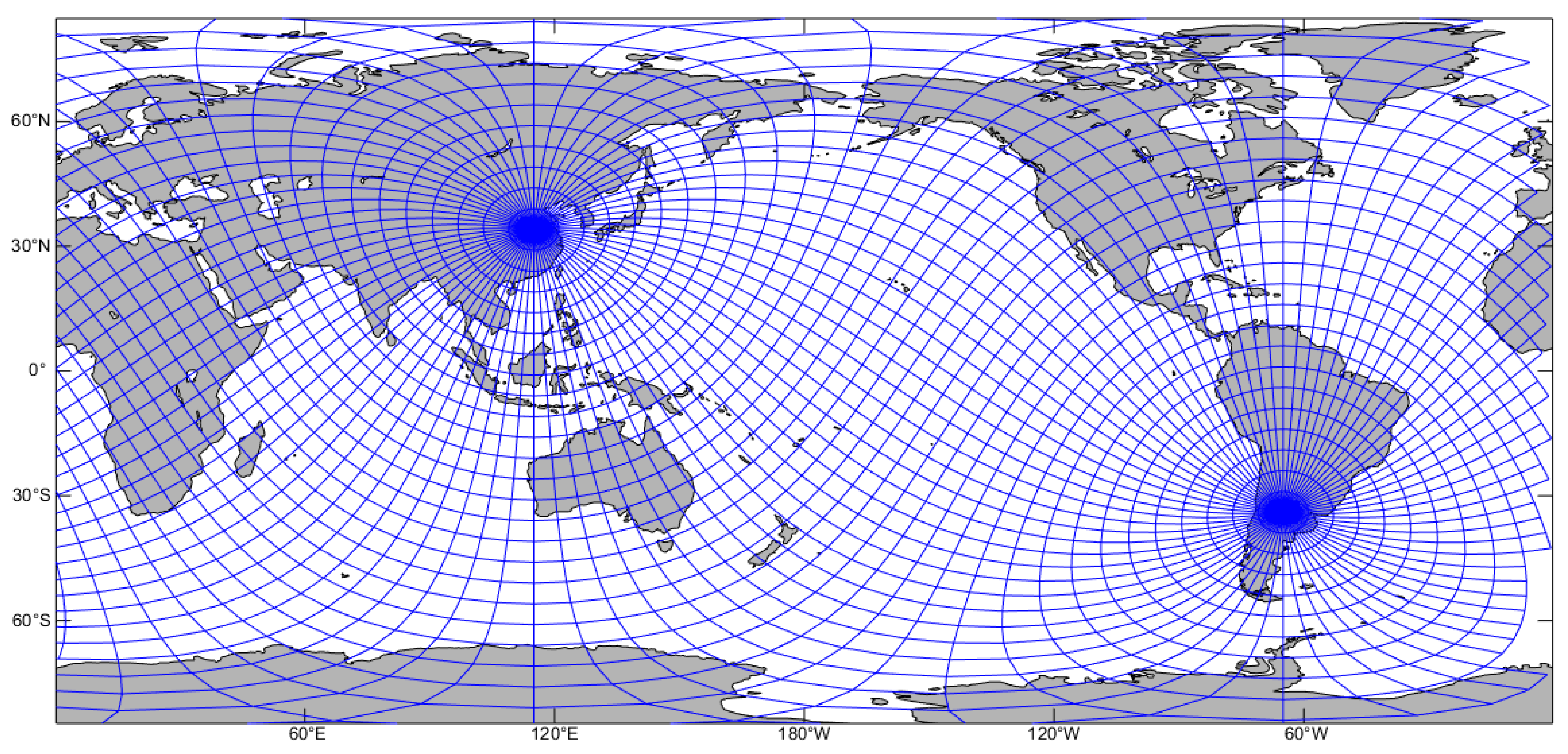
After a series of tests, it turns out that the poles can be shifted on the mainland in two ways, where one pair of anti-poles are in Eastern China and Argentina (a typical value is $\alpha =-60,\beta =0, \gamma =25$), and the other pair are in Greenland and Antarctica (a typical value is $\alpha =10,\beta =13, \gamma =0$), as shown in Figure 1 and Figure 2. The results of Tsunami simulation show that more accurate results can be achieved on the second mesh [26]. Hence, the mesh in Figure 2 was also preferred in this paper.

3. Model Formulation

On the spherical surface, the seawater movement described by shallow water wave equations must meet the following assumptions [14]:

• The Earth is considered a standard sphere, and the ocean has a free surface;
• Gravity is the main restoring force, and energy is dissipated by the friction between water flow and solid boundaries and by the internal friction between water flows of different velocities;
• The hydrostatic pressure assumption states that the acceleration of the flow velocity is relatively small in the vertical direction and that the pressure distribution of the water is close to the pressure distribution at the static state;
• The derivative of the horizontal flow velocity in the vertical direction is close to zero; that is, the difference between flow velocities is trivial in the vertical direction.

Under the conditions mentioned above and in spherical LL coordinates, the 2D tidal wave equations can be expressed in a flux form as follows [14,27]:

$$\frac{\partial \zeta }{\partial t}+\frac{1}{R\cos (\theta )}(\frac{\partial UH}{\partial \lambda }+\frac{\partial V\cos (\theta )H}{\partial \theta })=0$$

(3)

$$\begin{gathered} \frac{\partial UH}{\partial t}+\frac{1}{R\cos (\theta )}[\frac{\partial (U·UH)}{\partial \lambda }+\frac{\partial (V\cos (\theta )·UH)}{\partial \theta }]-\frac{U·VH}{R}\tan (\theta )-fVH \\ =-\frac{gH}{R\cos (\theta )}\frac{\partial (\zeta -{\zeta }_{EQ}-{\zeta }_{SAL})}{\partial \lambda }+\frac{{\tau }_{s\lambda }-{\tau }_{b\lambda }}{{\rho }_0}+F_U \end{gathered}$$

(4)

$$\begin{gathered} \frac{\partial VH}{\partial t}+\frac{1}{R\cos (\theta )}[\frac{\partial (U·VH)}{\partial \lambda }+\frac{\partial (V\cos (\theta )·VH)}{\partial \theta }]+\frac{U·UH}{R}\tan (\theta )+fUH \\ =-\frac{gH}{R}\frac{\partial (\zeta -{\zeta }_{EQ}-{\zeta }_{SAL})}{\partial \theta }+\frac{{\tau }_{s\theta }-{\tau }_{b\theta }}{{\rho }_0}+F_V \end{gathered}$$

(5)

where on the right sides of Equations (4) and (5), the terms $F_U$ and $F_V$ denote the horizontal diffusion effect, which is formulated as follows:

$$F_U=\frac{A_H}{R^2\cos (\theta )}[\frac{\partial \cos (\theta )FX}{\partial \theta }+\frac{\partial FY}{\partial \lambda }-\sin (\theta )FX]$$

(6)

$$F_V=\frac{A_H}{R^2\cos (\theta )}[-\frac{\partial \cos (\theta )FY}{\partial \theta }+\frac{\partial FX}{\partial \lambda }+\sin (\theta )FY]$$

(7)

where FX, FY are auxiliary terms:

$$FX=H(\frac{\partial U}{\partial \theta }+\frac{1}{\cos (\theta )}\frac{\partial V}{\partial \lambda }+U\tan (\theta )), FY=H(\frac{1}{\cos (\theta )}\frac{\partial U}{\partial \lambda }-\frac{\partial V}{\partial \theta }-V\tan (\theta ))$$

(8)

From the second term in the momentum equations, the terms represent the advection, space curvature, Coriolis force, pressure gradient, wind stress and bottom frictional stress, and horizontal diffusion effect. The symbols and meanings of the other important variables are listed in

Table 1. Symbols and meanings of variables in the equations.

Variable Symbol	Meaning
t	time
$(\lambda ,\theta )$	long-lat. Coordinates
$(U,V)$	Horizontal flow-vector along the LL coordinates
$\zeta$	Water surface elevation
${\zeta }_{EQ}$	Equilibrium tide height
${\zeta }_{SAL}$	Effects of ocean Self-attraction and Loading
$H$	Instantaneous total depth
$f$	Coriolis parameter
$g$	Gravitational acceleration
$R$	Mean radius of Earth
${\rho }_0$	Mean density of seawater
$A_H$	Horizontal diffusion coefficient
$({\tau }_{s\lambda },{\tau }_{s\theta })$	Surface wind stresses
$({\tau }_{b\lambda },{\tau }_{b\theta })$	Frictional stresses at the bottom

. The $\lambda ,\theta$ denote the longitude-latitude coordinates, and $U,V$ denote the zonal and meridional component of the horizontal flow vector, t denotes time, R, f, g denote the Earth’s mean radius, the Coriolis parameter and gravitational acceleration, respectively. The total water depth is $H=h+\zeta$, where h, $\zeta$ denote the bathymetry and water surface height at cell-center respectively. ${\zeta }_{EQ}$ denotes the equilibrium tide height, ${\zeta }_{SAL}$ denotes the ocean Self-attraction and Loading effects, ${\rho }_0$ denotes the mean density of seawater, and ${\tau }_{b\lambda },{\tau }_{b\theta }$ denote the frictional stresses at the bottom of ocean. $A_H$ denotes the horizontal diffusion coefficient. The symbols and meanings of the important variables are listed in Table 1.

For accurate and long-term simulation of global ocean tides, the effects of ocean self-attraction and loading (SAL) must be taken into account [28,29,30,31]. These effects include the deformation of the elastic ocean seafloor due to the weight of the water column, the changes in the tide potential caused by the redistribution of seawater quantities, and the combined effects of these factors. If complete and strict effects of seawater SAL on the tide are considered, calculations of the convolution of the tidal potential are involved [32,33]; thus, the equations become integro-differential equations, which greatly increases the amount of calculation in the model. A coarser approach is to use a scalar approximation [34], i.e., a simple scalar multiplied by the local tidal elevation: ${\zeta }_{SAL}=\beta \zeta$, where the scalar multiplier is $\beta =0.085$, $\beta =0.1$ or $\beta =0.12$. Generally, $0.08<\beta \le 0.12$. Compared with the calculation of the tidal potential convolution, this approximation method has lower precision, but the efficiency is much higher.

In this paper, only the astronomical tide is considered, and other external factors are neglected, such as the influence of meteorological factors. The quadratic bottom friction law is expressed as follows [35]:

$$({\tau }_{b\lambda },{\tau }_{b\theta })=Bfric\ast \left|\overrightarrow{U}\right|\overrightarrow{U}=Bfric\ast \sqrt{U^2+V^2}(U,V)$$

(9)

where $Bfric$ denotes the bottom friction coefficient.

After rotated mapping, the form of the equations remains unchanged, while the coordinates should be the transformed LL coordinates. All grid metrics, such as edge length, cell area and curvature terms could be calculated in the rotated LL coordinates directly, but for terms related to realistic LL coordinates, such as the Coriolis parameter and the tide-producing potential terms, the coordinates should be replaced by original LL coordinates.

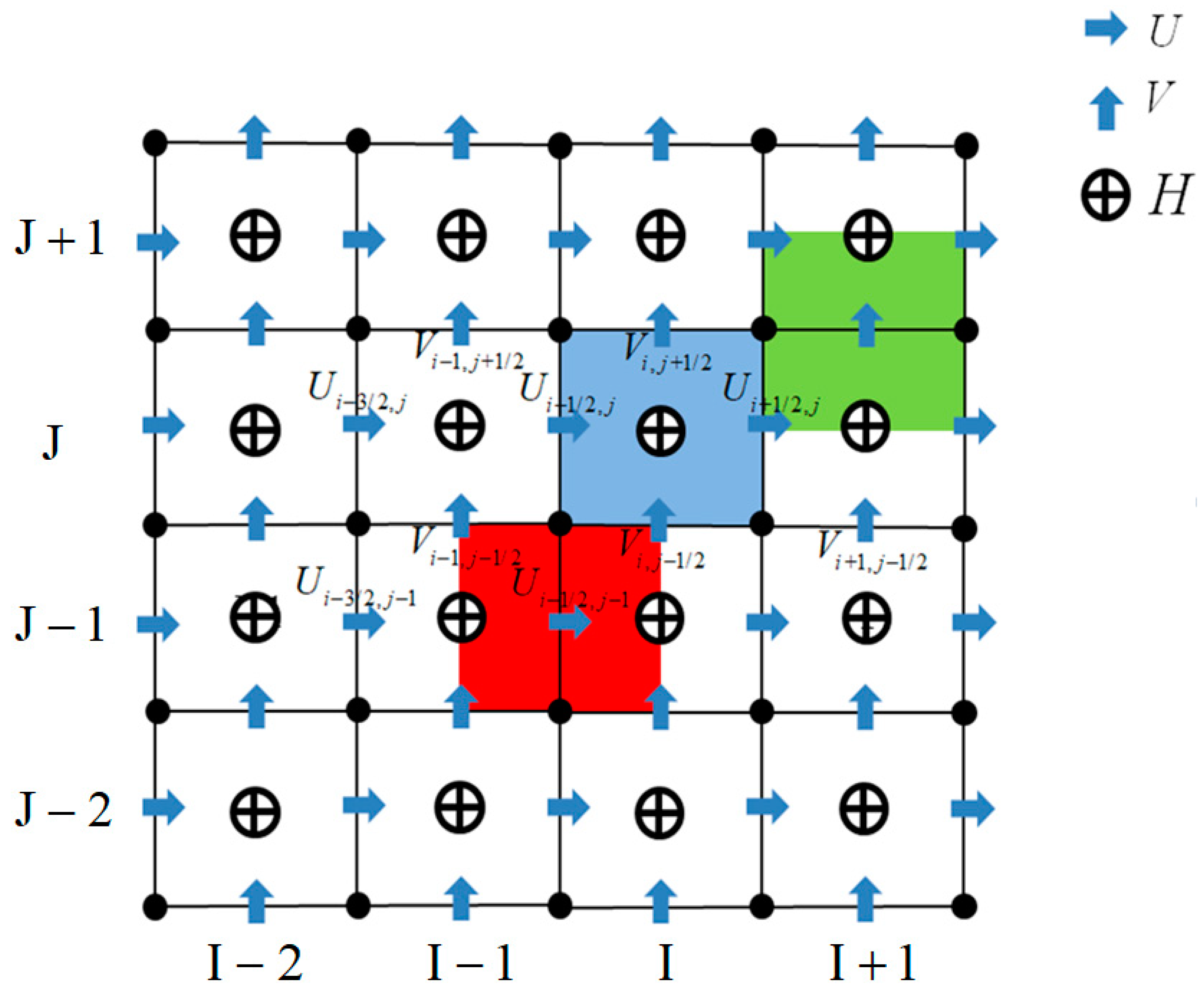
3.1. Spatial Discretization of Equations

For the numerical discretization of dynamical Equations (3)–(5) on the rotated LL grids, the Arakawa C-grid is preferable, because it has good dispersion properties of the inertia-gravity wave and gives an accurate representation of the geostrophic adjustment process provided that the Rossby deformational radius is well resolved [36]. The prognostic variables are discretized with the C-grid staggering as illustrated in Figure 3. The horizontal velocity normal to the cell edge (U or V) as a pointwise value is placed at the cell edges. The fluid thickness H is a cell-averaged value at cell-center. The quadrilaterals in red and green denote the control volume (${\mathsf{\Omega }}_U$, ${\mathsf{\Omega }}_V$) of horizontal velocity U, V, respectively.

3.1.1. Divergence Operator

The continuity equation (Equation (3)) is in flux form that guarantees mass conservation in the discrete system of equations; the mass-flux divergence can be given by using the Gauss divergence theorem over the cell

$${(\nabla ·(\overrightarrow{V}H))}_{i,j}=\frac{1}{A_{i,j}}\left[{(U{H}_{\mathrm{e}}\ast l)}_{i+1/2,j}-{(U{H}_{\mathrm{e}}\ast l)}_{i-1/2,j}+{(V{H}_{\mathrm{e}}\ast l)}_{i,j+1/2}-{(V{H}_{\mathrm{e}}\ast l)}_{i,j-1/2}\right]$$

(10)

where $\overrightarrow{V}=(U,V)$, $A_{i,j}$ and l denote the area and the edge length of the primary cell, respectively. The total depth at the cell edge He needs to be interpolated from the primal cell centers; for example, the total depth at the east edge of the cell is:

$${(H_e)}_{i+1/2,j}=\frac{H_{i,j}+H_{i+1,j}}{2},\begin{array}{cc}& H_{i,j}=h_{i,j}+{\zeta }_{i,j}\end{array}$$

(11)

where $H_{i,j}$ is the total water depth at cell-center. Grid metrics, such as the edge length $l$ and cell area $A_{i,j}$ can be approximated easily:

$$\begin{array}{l}{l}_{i+1/2,j}=R·\Delta \theta ,\begin{array}{cc}& l_{i,j+1/2}=R\cos ({\theta }_{j+1/2})·\Delta \lambda \end{array}\\ A_{i,j}=R^2(\sin ({\theta }_{j+1/2})-\sin ({\theta }_{j-1/2}))·\Delta \lambda \end{array}$$

(12)

where $\Delta \lambda$, $\Delta \theta$ are space resolution. Then the continuity equation could be discretized as follows:

$${(\frac{\partial \zeta }{\partial t})}_{i,j}+{(\nabla ·(\overrightarrow{V}H))}_{i,j}=0$$

(13)

3.1.2. Reconstruction of Tangent Velocity

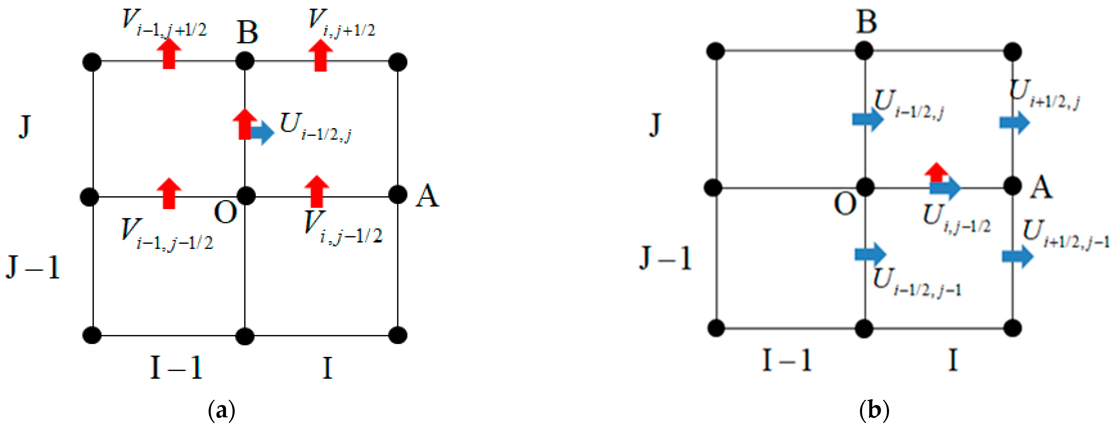
It is obvious that only the normal velocity is placed at each cell edge; in order to calculate the full advection flux terms, the Coriolis and curvature terms in the momentum Equations (4) and (5), the tangent velocity component on each edge is needed.

There are several methods to reconstruct the tangent velocity on cell edges, such as polynomial fitting or least-square fitting, interpolation based on edge finite element (RT0 element) or based on RBF(radial basis function) [37,38], etc.; here bi-linear polynomial interpolation was utilized. As shown in Figure 4a, on the edge OB, the tangent velocity is:

$$\begin{array}{l}{\overline{V}}_{i-1/2,j}\approx \frac{{(VH)}_{i,j}+{(VH)}_{i-1,j}}{2H_{i-1/2,j}}\\ \approx \frac{({(VH)}_{i,j}{}_{+1/2}+{(VH)}_{i,j-1/2})/2+({(VH)}_{i-1,j}{}_{+1/2}+{(VH)}_{i-1,j-1/2})/2}{2H_{i-1/2,j}}\end{array}$$

(14)

Similarly, on the edge OA shown in Figure 4b, the tangent velocity is:

$$\begin{array}{l}{\overline{U}}_{i,j-1/2}\approx \frac{{(UH)}_{i,j}+{(UH)}_{i,j-1}}{2H_{i,j-1/2}}\\ \approx \frac{({(UH)}_{i-1/2,j}+{(UH)}_{i+1/2,j})/2+({(UH)}_{i-1/2,j-1}+{(UH)}_{i+1/2,j-1})/2}{2H_{i,j-1/2}}\end{array}$$

(15)

3.1.3. Approximation of Momentum Equations

First, the momentum Equation (4) is integrated on the control volume ${\mathsf{\Omega }}_U$ and Equation (5) is integrated on control volume ${\mathsf{\Omega }}_V$ respectively; detailed procedures for each term are given below.

Discretization of Advection Flux Terms

For the advection flux terms in Equation (4), a 1-order upwind scheme was utilized, yielding:

$$\begin{array}{l}\frac{1}{R\cos (\theta )}{\left[\frac{\partial (U·UH)}{\partial \lambda }+\frac{\partial (V\cos (\theta )·UH)}{\partial \theta }\right]}_{i-1/2,j}\\ \approx \frac{1}{R\cos ({\theta }_{i-1/2,j})}\left[\left(\frac{U_{i,j}+\left|U_{i,j}\right|}{2}{(UH)}_{i-1/2,j}+\frac{U_{i,j}-\left|U_{i,j}\right|}{2}{(UH)}_{i+1/2,j}\right)-\left(\frac{U_{i-1,j}+\left|U_{i-1,j}\right|}{2}{(UH)}_{i-3/2,j}+\frac{U_{i-1,j}-\left|U_{i-1,j}\right|}{2}{(UH)}_{i-1/2,j}\right)\right]\\ +\frac{1}{R\cos ({\theta }_{i-1/2,j})}\left(\frac{{(V\cos (\theta ))}_{i-1/2,j+1/2}+\left|{(V\cos (\theta ))}_{i-1/2,j+1/2}\right|}{2}{(UH)}_{i-1/2,j}+\frac{{(V\cos (\theta ))}_{i-1/2,j+1/2}-\left|{(V\cos (\theta ))}_{i-1/2,j+1/2}\right|}{2}{(UH)}_{i-1/2,j+1}\right)\\ -\frac{1}{R\cos ({\theta }_{i-1/2,j})}\left(\frac{{(V\cos (\theta ))}_{i-1/2,j-1/2}+\left|{(V\cos (\theta ))}_{i-1/2,j-1/2}\right|}{2}{(UH)}_{i-1/2,j-1}+\frac{{(V\cos (\theta ))}_{i-1/2,j-1/2}-\left|{(V\cos (\theta ))}_{i-1/2,j-1/2}\right|}{2}{(UH)}_{i-1/2,j}\right)\end{array}$$

(16)

Similarly, for the advection flux terms in Equation (5), yielding:

$$\begin{array}{l}\frac{1}{R\cos (\theta )}{\left[\frac{\partial (U·VH)}{\partial \lambda }+\frac{\partial (V\cos (\theta )·VH)}{\partial \theta }\right]}_{i,j-1/2}\\ \approx \frac{1}{R\cos ({\theta }_{i,j-1/2})}\left[\left(\frac{U_{i+1/2,j-1/2}+\left|U_{i+1/2,j-1/2}\right|}{2}{(VH)}_{i,j-1/2}+\frac{U_{i+1/2,j-1/2}-\left|U_{i+1/2,j-1/2}\right|}{2}{(VH)}_{i+1,j-1/2}\right)-\left(\frac{U_{i-1/2,j-1/2}+\left|U_{i-1/2,j-1/2}\right|}{2}{(VH)}_{i-1,j-1/2}+\frac{U_{i-1/2,j-1/2}-\left|U_{i-1/2,j-1/2}\right|}{2}{(VH)}_{i,j-1/2}\right)\right]\\ +\frac{1}{R\cos ({\theta }_{i,j-1/2})}\left(\frac{{(V\cos (\theta ))}_{i,j}+\left|{(V\cos (\theta ))}_{i,j}\right|}{2}{(VH)}_{i,j-1/2}+\frac{{(V\cos (\theta ))}_{i,j}-\left|{(V\cos (\theta ))}_{i,j}\right|}{2}{(VH)}_{i,j+1/2}\right)\\ -\frac{1}{R\cos ({\theta }_{i,j-1/2})}\left(\frac{{(V\cos (\theta ))}_{i,j-1}+\left|{(V\cos (\theta ))}_{i,j-1}\right|}{2}{(VH)}_{i,j-3/2}+\frac{{(V\cos (\theta ))}_{i,j-1}-\left|{(V\cos (\theta ))}_{i,j-1}\right|}{2}{(VH)}_{i,j-1/2}\right)\end{array}$$

(17)

where the velocity at cell-center is approximated as:

$$U_{i,j}\approx \frac{U_{i-1/2,j}+U_{i+1/2,j}}{2},\begin{array}{cc}& \end{array}{V}_{i,j}\approx \frac{V_{i,j-1/2}+V_{i,j+1/2}}{2}$$

(18)

Discretization of Coriolis Curvature Terms

In the momentum equations, the curvature and Coriolis terms are approximated by the average of values at two neighbor cells sharing a common edge.

$$\begin{gathered} {(\frac{U·VH}{R}\tan (\theta )+fVH)|}_{i-1/2,j}\approx \frac{{(VH)}_{i-1,j}+{(VH)}_{i,j}}{2}[\frac{{(\tan (\theta )·U)}_{i-1,j}+{(\tan (\theta )·U)}_{i,j}}{2R}+f_{i-1/2,j}] \\ {(\frac{U·UH}{R}\tan (\theta )+fUH)|}_{i,j-1/2}\approx \frac{{(UH)}_{i,j-1}+{(UH)}_{i,j}}{2}[\frac{{(\tan (\theta )·U)}_{i,j-1}+{(\tan (\theta )·U)}_{i,j}}{2R}+f_{i,j-1/2}] \end{gathered}$$

(19)

Discretization of Normal Gradient

In the momentum equations (Equations (4) and (5)), to calculate ∂UH/∂t, ∂VH/∂t, one needs to discretize the gradient of geopotential on the primal cell edge. On the long-lat. grid, the edge of the primal cell is perpendicular to and bisected by the edge of the dual cell; hence, the second-order central finite-difference method can be implemented straightforwardly. For example, on the edge OB and OA in Figure 4, the gradients of geopotential in the zonal and meridional direction are calculated as

$$\begin{gathered} {\frac{H}{R\cos (\theta )}\frac{\partial \zeta }{\partial \lambda }|}_{i-1/2,j}\approx H_{i-1/2,j}\frac{{\zeta }_{i,j}-{\zeta }_{i-1,j}}{R\cos ({\theta }_j)·\Delta \lambda } \\ {\frac{H}{R}\frac{\partial \zeta }{\partial \theta }|}_{i,j-1/2}\approx H_{i,j-1/2}\frac{{\zeta }_{i,j}-{\zeta }_{i,j-1}}{R·\Delta \theta } \end{gathered}$$

(20)

Discretization of Diffusion Terms

The horizontal diffusion terms in the momentum equations (Equations (4) and (5)) denote the internal friction effects between water particles of different velocities. They are discretized as follows:

$$\begin{array}{l}{F_U|}_{i-1/2,j}={\frac{A_H}{R^2\cos (\theta )}[\frac{\partial \cos (\theta )FX}{\partial \theta }+\frac{\partial FY}{\partial \lambda }-\sin (\theta )FX]|}_{i-1/2,j}\\ \approx \frac{A_H}{R^2\cos ({\theta }_j)}[\frac{\cos ({\theta }_{j+1/2})F{X}_{i-1/2,j+1/2}-\cos ({\theta }_{j-1/2})F{X}_{i-1/2,j-1/2}}{\Delta \theta }+\frac{F{Y}_{i,j}-F{Y}_{i-1,j}}{\Delta \lambda }-\sin ({\theta }_j)\frac{F{X}_{i-1/2,j+1/2}+F{X}_{i-1/2,j-1/2}}{2}]\end{array}$$

(21)

$$\begin{array}{l}{F_V|}_{i,j-1/2}{=\frac{A_H}{R^2\cos (\theta )}[-\frac{\partial \cos (\theta )FY}{\partial \theta }+\frac{\partial FX}{\partial \lambda }+\sin (\theta )FY]|}_{i,j-1/2}\\ \approx \frac{A_H}{R^2\cos ({\theta }_{j-1/2})}[\frac{\cos ({\theta }_{j-1})F{Y}_{i,j-1}-\cos ({\theta }_j)F{Y}_{i,j}}{\Delta \theta }+\frac{F{X}_{i+1/2,j-1/2}-F{X}_{i-1/2,j-1/2}}{\Delta \lambda }+\sin ({\theta }_{j-1/2})\frac{\cos ({\theta }_j)F{Y}_{i,j}+\cos ({\theta }_{j-1})F{Y}_{i,j-1}}{2}]\end{array}$$

(22)

where the auxiliary term $FX$ is placed at node and $FY$ at cell-center, which are approximated as follows:

$$\begin{array}{l}FX={H(\frac{\partial U}{\partial \theta }+\frac{1}{\cos (\theta )}\frac{\partial V}{\partial \lambda }+U\tan (\theta ))|}_{i-1/2,j-1/2}\\ \approx \frac{H_{i,j}+H_{i-1,j}+H_{i-1,j-1}+H_{i,j-1}}{4}(\frac{U_{i-1/2,j}-U_{i-1/2,j-1}}{\Delta \theta }+\frac{V_{i,j-1/2}-V_{i-1,j-1/2}}{\cos ({\theta }_{j-1/2})\Delta \lambda }+\frac{U_{i-1/2,j}+U_{i-1/2,j-1}}{2}\tan ({\theta }_{j-1/2})\end{array}$$

(23)

$$\begin{array}{l}FY={H(\frac{1}{\cos (\theta )}\frac{\partial U}{\partial \lambda }-\frac{\partial V}{\partial \theta }-V\tan (\theta ))|}_{i,j}\\ \approx H_{i,j}(\frac{U_{i+1/2,j}-U_{i-1/2,j}}{\cos ({\theta }_j)\Delta \lambda }-\frac{V_{i,j+1/2}-V_{i,j-1/2}}{\Delta \theta }-\frac{V_{i,j+1/2}+V_{i,j-1/2}}{2}\tan ({\theta }_j))\end{array}$$

(24)

3.2. Time Integration

In the real world, ocean tidal dynamics are a continuous time-space process, so it is necessary to figure out an efficient time-stepping scheme for numerical simulations. Although implicit time integration is beneficial to the stability of the model run, it costs much more time because it requires the solving of large-scale nonlinear equations. In this model, a generalized forward-backward (FB) scheme would be used, which is a combination of a third-order Adams-Bashforth (AB3) method with a fourth-order Adams-Moulton (AM4) method [39,40], which is referred to as the “AB3-AM4 FB scheme”. However, this scheme is slightly modified for the friction at the bottom [14]. Essentially, the method is a prediction-correction scheme. The time integration is divided into three major parts as follows:

Step 1: First, the AB3 method is used to extrapolate the elevation and the flow vectors in the time level $n+\frac{1}{2}$:

$$\begin{array}{l}{\zeta }^{n+\frac{1}{2}}=(1+\alpha +\beta ){\zeta }^n-(\alpha +2\beta ){\zeta }^{n-1}+\beta {\zeta }^{n-2}\\ U^{n+\frac{1}{2}}=(1+\alpha +\beta )U^n-(\alpha +2\beta )U^{n-1}+\beta U^{n-2}\\ V^{n+\frac{1}{2}}=(1+\alpha +\beta )V^n-(\alpha +2\beta )V^{n-1}+\beta V^{n-2}\end{array}$$

(25)

It can be seen that the extrapolated value of each component equals its weighted average value over the previous three time intervals. Furthermore, the parameters $(\alpha ,\beta )$ can be set to many different values; here, the values $(\alpha ,\beta )=(0.5,0.281105)$ have been chosen because they improve the stability of the scheme.

Step 2: The continuity equation is solved for the water elevation in the next time interval, and the divergence operator can be approximated according to Equation (10), yielding:

$${\zeta }^{n+1}={\zeta }^n-dt\ast \mathrm{flux}({\zeta }^{n+\frac{1}{2}},U^{n+\frac{1}{2}},V^{n+\frac{1}{2}})$$

(26)

where “flux” is the mass flux across the boundary of the mass control volume. Then the water elevation ${\zeta }^{n+1}$ is corrected by the AM4 method, and the corrected value is denoted ${\tilde{\zeta }}^{n+1}$, that is:

$${\tilde{\zeta }}^{n+1}=(0.5+\gamma +2\epsilon ){\zeta }^{n+1}+(0.5-2\gamma -3\epsilon ){\zeta }^n+\gamma {\zeta }^{n-1}+\epsilon {\zeta }^{n-2}$$

(27)

where parameters $(\gamma ,\epsilon )=(0.088,0.013)$ yield a good stability range for the wave system while maintaining monotonically increasing dissipation [40]. Additionally, it is subsequently necessary to update the constant total depth, which is used in the discretization of barotropic gradient terms in the momentum equations.

Step 3: The momentum equations are solved for each flow vector component in the next time interval. The curvature, Coriolis, advection and diffusion terms are calculated based on the values in time level $n+\frac{1}{2}$, and the bottom friction term is processed semi-implicitly:

$$\begin{gathered} U^{n+1}{H}^{n+1}={(UH)}^n+dt\ast [{\mathrm{baro}}^{\mathrm{AM}4}+{\mathrm{advect}}^{\mathrm{n}+\frac{1}{2}}{+(\mathrm{curvature}+\mathrm{coriolis})}^{\mathrm{n}+\frac{1}{2}}{+\mathrm{diffusion}}^{\mathrm{n}+\frac{1}{2}}]-dt\ast ({\mathrm{bottom}}^{n+\frac{1}{2}})\ast U^{n+1} \\ {V}^{n+1}{H}^{n+1}={(VH)}^n+dt\ast [{\mathrm{baro}}^{\mathrm{AM}4}+{\mathrm{advect}}^{\mathrm{n}+\frac{1}{2}}{+(\mathrm{curvature}+\mathrm{coriolis})}^{\mathrm{n}+\frac{1}{2}}{+\mathrm{diffusion}}^{\mathrm{n}+\frac{1}{2}}]-dt\ast ({\mathrm{bottom}}^{n+\frac{1}{2}})\ast V^{n+1} \end{gathered}$$

(28)

where $dt$ denotes the time-step; starting from the first term in the brackets, the discrete barotropic pressure gradient term, advection term, curvature term, Coriolis term, and diffusion term are represented respectively; the last represents the bottom friction term; and the superscript denotes the time-level.

3.3. Wetting and Drying Judgment

In numerical models for ocean modelling, an important phenomenon that should be addressed with special numerical methods is wetting and drying (WAD), which normally occurs in low-lying coastal zones, embayments and inlets. This process should be reflected in each tidal model, such as the well-known POM model [41,42] and the FVCOM model [43], and some studies have been performed on evaluations of WAD [44]. Essentially, the WAD algorithm is closely related to the numerical model that it serves, and it heavily depends on the specified discretization methods used in the model, therefore it is difficult to be extended to general cases.

A robust WAD scheme should not only maintain the stability and mass balance but also precisely reflect the real physical process. Naturally, the total water depth at cell-center is considered, and a threshold value, the minimal water depth $D_{\min }$ (commonly approximately 10 cm), is set in advance. The cell would be judged as in a wet state if its total water depth $H$ is equal to or greater than $D_{\min }$; otherwise, the cell is dry. Then the WAD of normal velocity at edges can be judged according to that of the cells which share this edge.

The control volume for $U_{i-1/2,j}$ is wet in the following two cases:

(1)

If cell(i−1,j) is wet and cell(i,j) is wet.

(2)

Only one cell, cell(i−1,j) or cell(i,j), is wet, and the barotropic gradient on the common edge shared by the two cells is not zero.

Similarly, the control volume for $V_{i,j-1/2}$ is wet in the following two cases:

(1)

If cell(i,j−1) is wet and cell(i,j) is wet.

(2)

Only one cell, cell(i,j−1) or cell(i,j), is wet, and the barotropic gradient on the common edge shared by the two cells is not zero.

4. Numerical Experiments

As a validation, we show the application of the model to the simulation of tidal dynamics in the global ocean. As shown in Figure 5a, the computational domain was discretized by the rotated LL grids in Mercator projection, and Figure 5b shows the grids in the region close to the North pole in stereographic projection. Once the grids were generated, the bathymetry at each cell-center was attained from the ETOPO2 data by bilinear interpolation. The mean radius of the Earth (R) was taken as 6371.393 km and gravitational acceleration (g) was assumed to be 9.81 m/s². The mean density of seawater was assumed to be 1025 kg/m³ and the horizontal diffusion coefficient was set to be 10⁴ m²/s. The model is run with a spatial resolution of 0.5 degrees, the time step is set to 15 s, and the bottom friction coefficient is 0.004 if the water depth exceeds 1000 m and 0.005 otherwise. The computation domain was forced by eight major tide constituents, including four semidiurnal tide constituents and four diurnal tide constituents, which are typically written as M₂, S₂, N₂, K₂, K₁, O₁, P₁ and Q₁. The model was started from a static ocean, that is, the initial values of surface height and horizontal flow-vector are all zeros. Period boundary conditions are exerted on the east and west boundaries, and the normal flux across the edge is set as zero if it is shared by land and ocean cells. We run the model for 33 model days, and then the time series of water surface elevation at each cell-center was fitted by the least squares harmonic analysis method.

4.1. Accuracy Evaluation

There are several methods to assess the accuracy of an ocean tide model, the most popular being a comparison of the modelling results with the data obtained from tide gauges or satellite altimetry (i.e., reference truth values). Generally, the tidal harmonic constants are used as basic data. The evaluation was made by computing the RMS (root mean square) difference of harmonic constants for each reference truth data, which is defined as [45]:

$$RM{S}_k=\sqrt{\frac{1}{2N}{\displaystyle \sum _{j=1}^N\{{[{\widehat{C}}_k(j)\cos {\widehat{\phi }}_k(j)-C_k(j)\cos {\phi }_k(j)]}^2+{[{\widehat{C}}_k(j)\sin {\widehat{\phi }}_k(j)-C_k(j)\sin {\phi }_k(j)]}^2\}}}$$

(29)

where $C_k(j),{\phi }_k(j)$ are the amplitude and Greenwich phase for tidal constituent k from numerical modelling, and ${\widehat{C}}_k(j),{\widehat{\phi }}_k(j)$ are their counterparts from the reference truth data for each location j. $N$ is the number of the spatial locations involved. The variable $RM{S}_k$ has the same unit as amplitude.

A common dataset for tidal reference truth values is the ST102 data set [46], providing the tidal harmonic constants of 102 sites which are rather regularly distributed over the world’s oceans. Another dataset is that of the ocean bottom pressure records with 66 sites (https://www.psmsl.org/data/bottom_pressure/table.php, 2 August 2021). Another dataset is GLOSS network (https://www.gloss-sealevel.org/gloss-station-handbook, 2 August 2021) which includes 290 sites. Figure 6 shows the location of each site, in which the blue plus denotes the site in the ST102 dataset, the blue solid triangle denotes the site in the ocean bottom pressure records and the red dot denotes the site in the GLOSS network, respectively. However, the original tidal harmonic constants from these observation sites are not available readily; instead, we utilized six well-known tide models for reference truth data, including FES2004, GOT4.8, TPXO7, DTU10, EOT11a, HAMTIDE12 (http://ftp.legos.obs-mip.fr/pub/FES2012-project/data/tides, 2 August 2021). These models are often chosen as reference data [4], and for each site in the ST102 data set, bottom pressure records and the GLOSS network, the harmonic constants could be extracted from the results of these six models by bilinear interpolation.

According to Equation (29), we compute the RMS for two major semidiurnal tide constituents M2, S2 and two diurnal tide constituents K1, O1 for the above three datasets, respectively. Figure 7 shows the RMS between the proposed model and the other six global tidal models for each gauge dataset; it is clear that the RMS has nearly the same order of magnitude for the ST102 and Bot66 dataset. For M2 and S2, the RMS is not more than 40 cm and 30 cm, except for the GOT4.8 and TPXO7 model; for K1 and O1, the RMS is not more than 30 cm and 25 cm.

In comparison with the ST102 and Bot66 datasets, the value of RMS is relatively larger in the GLOSS network for all six tide models. There are two main reasons for this difference; the tide amplitude is higher in coastal regions than that in deep ocean generally, and most sites in the first two datasets are located in deep ocean, which is less affected by the space resolution and complex coastal geography.

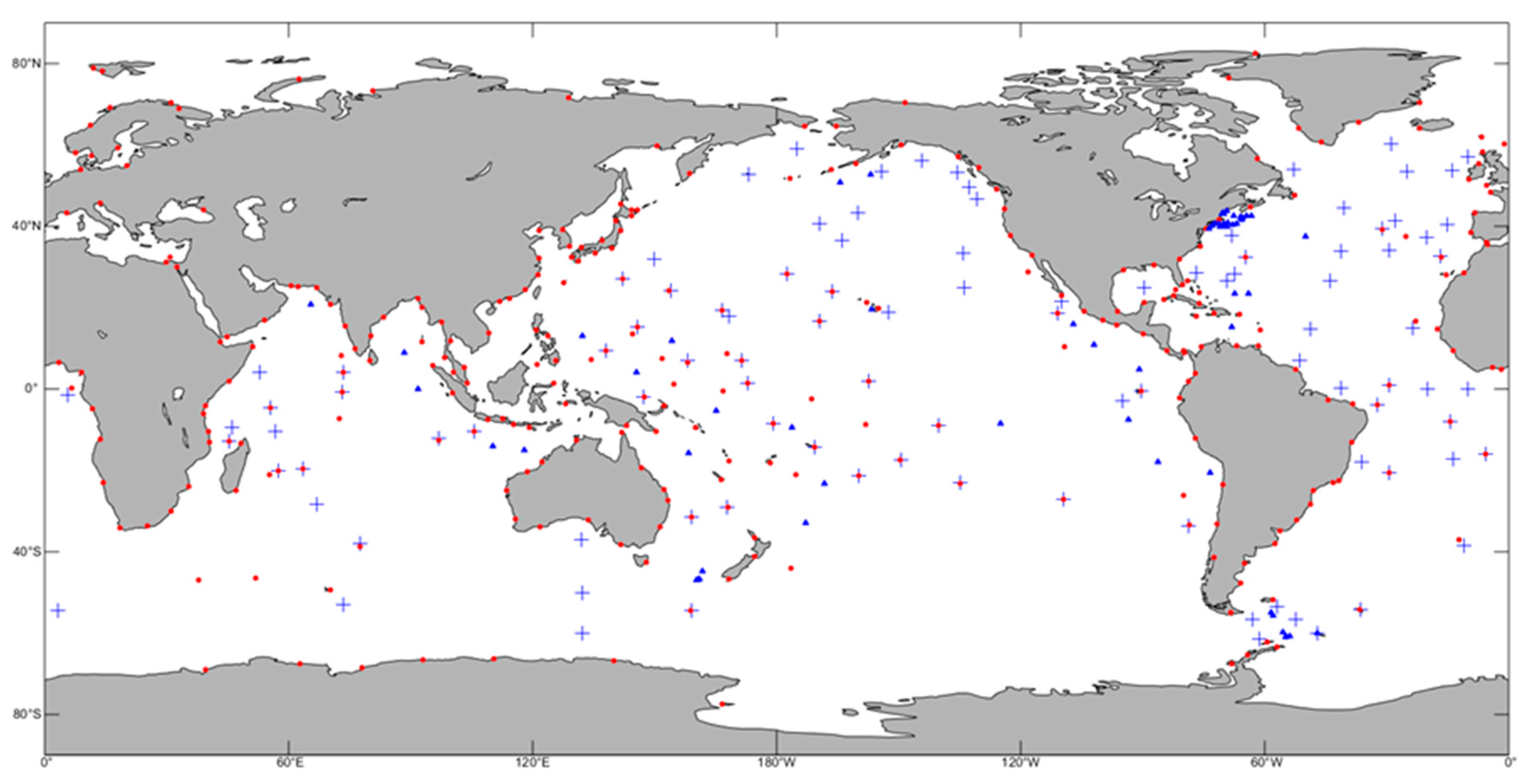
Obviously, most of the sites in the above three data sets are located in mid- and low latitude regions. It is difficult to implement the accuracy assessment of modelling results in the Arctic Ocean for lack of an authenticated gauge data set, as the number of accurate and reliable data sets for in situ tidal observations is quite limited [47]. A commonly used dataset for tide gauge data can be downloaded from http://www.ims.uaf.edu/tide/, December 2015, and from Kowarlik and Proshutinsky [48,49,50]. The gauge dataset includes 297 stations, whose positions are shown in Figure 8; it is obvious that most of sites are in coastal regions. Unfortunately, the harmonic constants in many sites are missing and the quality of data is not desirable; instead, the harmonic constants could be extracted from the results of these six models by bilinear interpolation for each station of the dataset. To a large extent, these interpolated results could be seen as reference truth data.

Figure 9 shows the RMS between the proposed model and the other six global tidal models for the gauge dataset in the Arctic Ocean. It is clear that the RMS is not more than 45 cm for M₂ and S₂ constituents; the RMS is not more than 40 cm for K₁ and 35 cm for O₁ except for the EOT11a and Hamtide12 model.

In view of the relatively low space resolution and lack of data assimilation, the current modelling result may not archive the same precision as other well-developed models, while the newly proposed method is capable of building a workable ocean tide model with reasonable accuracy, and it is hopeful that the accuracy of the presented model could be further improved by increasing the space resolution or adding data assimilation.

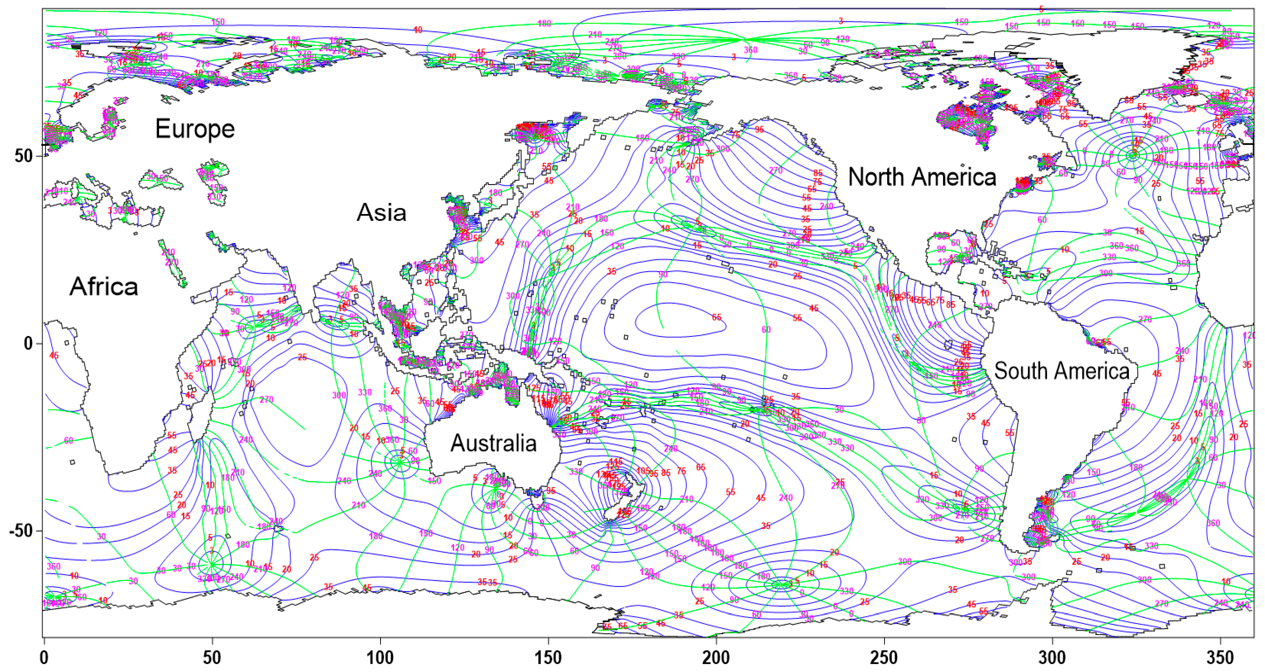
4.2. Co-Tidal Map in the Global Ocean

The resulting co-amplitude and co-phase lines of each tide constituent are shown in Figure 10, Figure 11, Figure 12 and Figure 13 (co-amplitude lines are shown as blue solid lines, and the number labels are shown as red lines. Co-phase lines are shown as green solid lines, and the number labels are shown in magenta). These figures show that the tidal wave propagates onto the continental shelf from the deep ocean. The tidal dynamics in the marginal sea of the continental shelf are forced by those of the adjacent deep ocean and are influenced by the coastline-induced reflection and refraction of the tidal wave.

For the major semidiurnal tide constituents, such as the M₂ and S₂ tides, the model predicts more than ten amphidromic points, of which four are located in the eastern and southern Pacific Ocean, two are located in the western Pacific Ocean, three are located in the Atlantic Ocean, and two are located in the Indian Ocean. In addition, it can also be seen from Figure 11 that the pattern of the S₂ tide is very similar to that of M₂ (shown in Figure 10), with only minor discrepancy in the details.

For the major diurnal tide constituents, such as the K₁ and O₁ tides, the model predicts three amphidromic points in the Pacific Ocean, two in the Atlantic Ocean, and one in the Indian Ocean. It can be seen that amphidromic systems are anticlockwise in the north hemisphere, and clockwise in the south hemisphere. Similarly, the pattern of the O₁ tide (shown in Figure 13) is similar to that of K₁ (shown in Figure 12), but its amplitude is smaller.

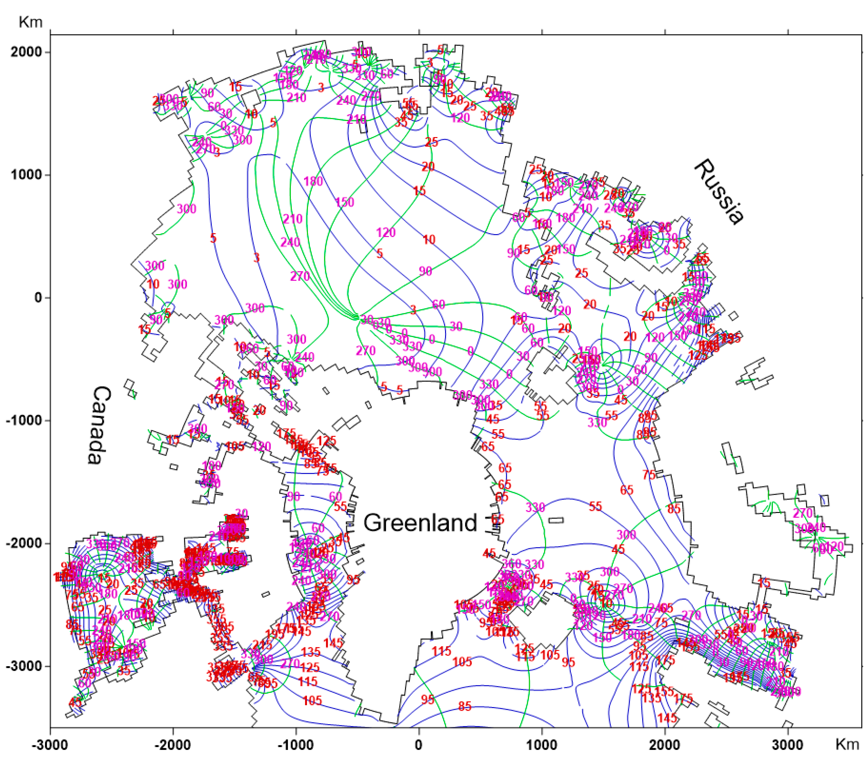
4.3. Co-Tidal Map in the Arctic Ocean

The tides in the Arctic Ocean have an effect on those in the adjacent marginal seas and the North Atlantic Ocean. Figure 14 shows the co-tidal map of the M₂ component in the Arctic Ocean under the stereographic coordinates. In all, seven distinct amphidromic points were obtained. Although the position of an amphidromic point may be drifted off the right location, the model reproduces the largest counterclockwise system off the northwest of the Queen Elizabeth Islands for M₂ constituent, one amphidromic point in the Davis Strait, one in the Kara Sea, one in the Barents Sea, one in the east nearshore of the Iceland, one in the Denmark Strait, and two in the Hudson Bay. The amplitude of the M₂ tide is generally no more than 120 cm, except for that in the near-shore of the Barents Sea and the marginal region adjacent to the North Atlantic Ocean.

The co-tidal map of the S₂ component is given in Figure 15. In general, it is very similar to that of the M₂ constituent in terms of the position and shape of the node points, but the amplitude is smaller; in most areas, it is no more than 60 cm except for that in the marginal region adjacent to the North Atlantic Ocean.

The co-tidal maps of the diurnal tide constituents K₁ and O₁ are given in Figure 16 and Figure 17. Generally, the patterns are not regular. Three amphidromic points were identified, one in the Kara Sea, one in the Barents Sea and one in the Hudson Bay. In general, the amplitude of the K₁ and O₁ constituents is no more than 30 cm except that in the Davis Strait in the west of Greenland.

5. Conclusions

A longitude-latitude grid combined with rotated coordinate transformation was developed to circumvent the “pole problem” in the Arctic regions in a global ocean numerical model. Then, the finite volume method was built to address the shallow water equations that accounted for the tidal potential of the eight main tide components, including the four major diurnal and semidiurnal constituents. The AB3-AM4 method is used for time integration. Based on orthogonality of the mesh, the model is straightforward and efficient, as it maintains the conservation of the total mass of the seawater. In general, the model has the capability of reproducing the basic spatial characteristics of ocean tidal dynamics, and a three dimensional model coupled with temperature and salt transport process will be developed in future.