
A New Normalized Groundwater Age-Based Index for Quantitative Evaluation of the Vulnerability to Seawater Intrusion in Coastal Aquifers: Implications for Management and Risk Assessments


Abstract
:1. Introduction
2. Background and Analysis of the Vulnerability Methods
3. Method Design and Development
3.1. Simulation of Coupled Variable-Density Flow and Transport
3.2. Simulation of Groundwater Age and the Vulnerability Index Development
4. Results
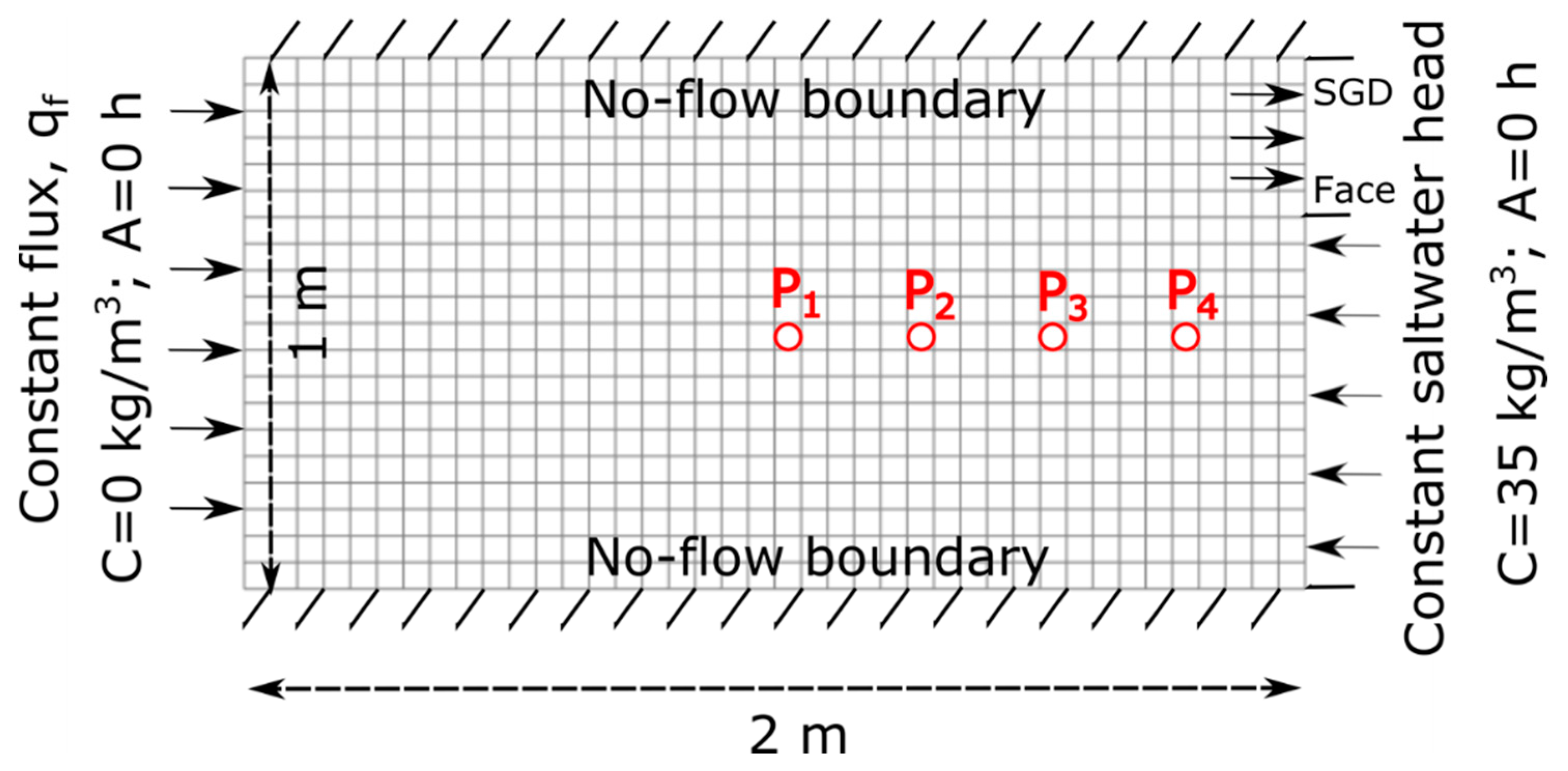
4.1. Example 1: The Henry Problem (Homogeneous and Heterogeneous Domains)
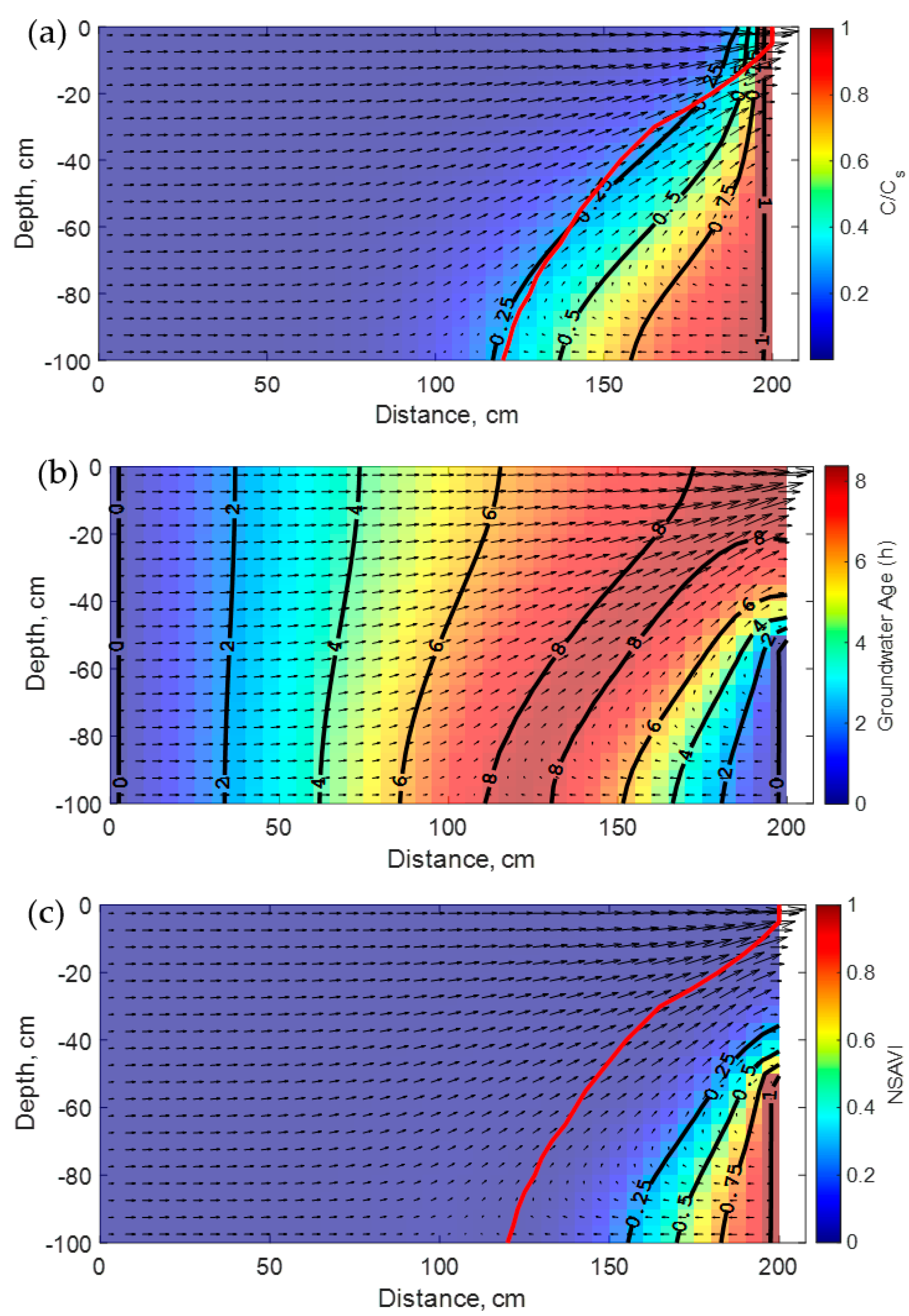
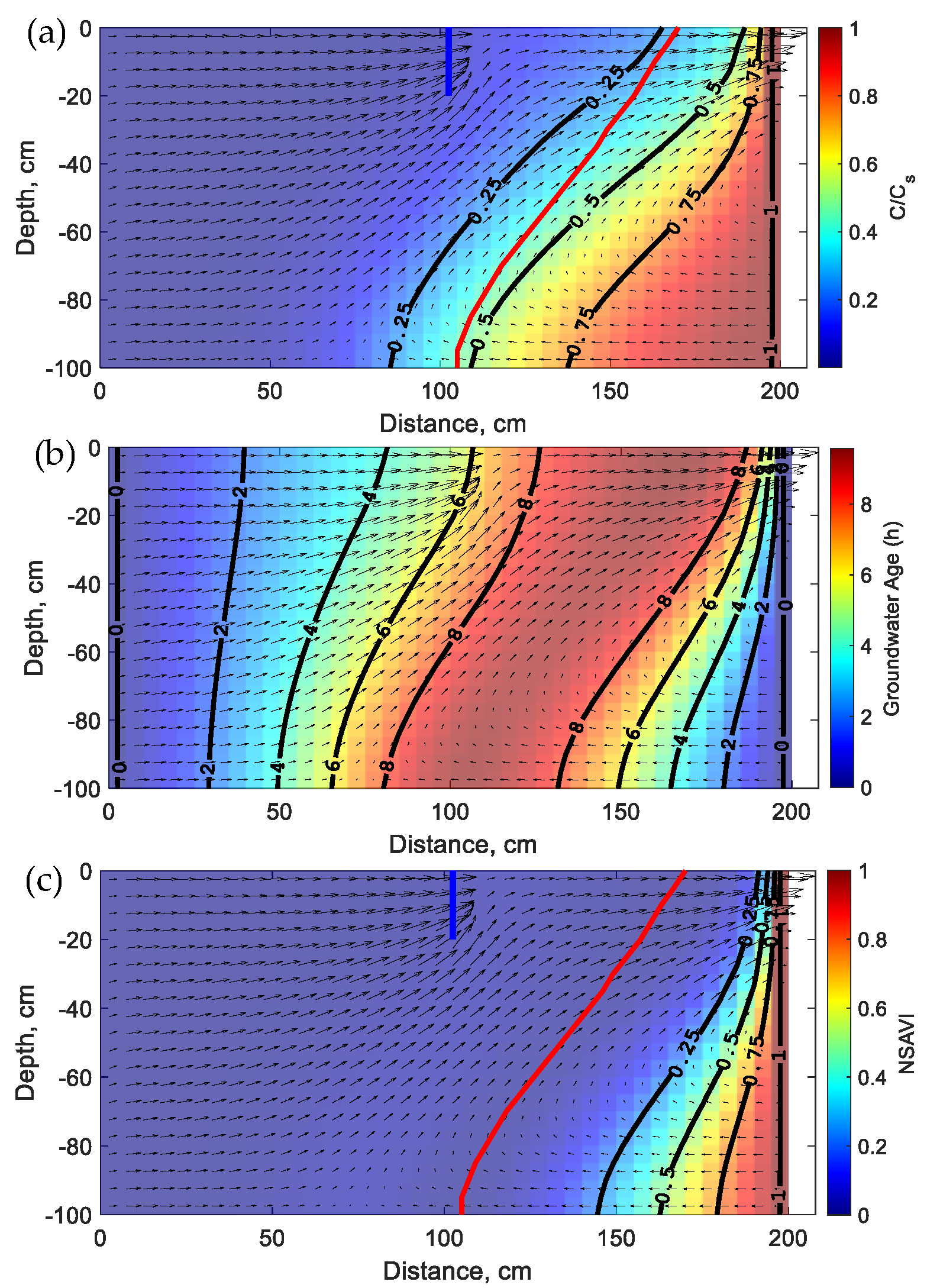
4.1.1. The Diffusive Henry Problem
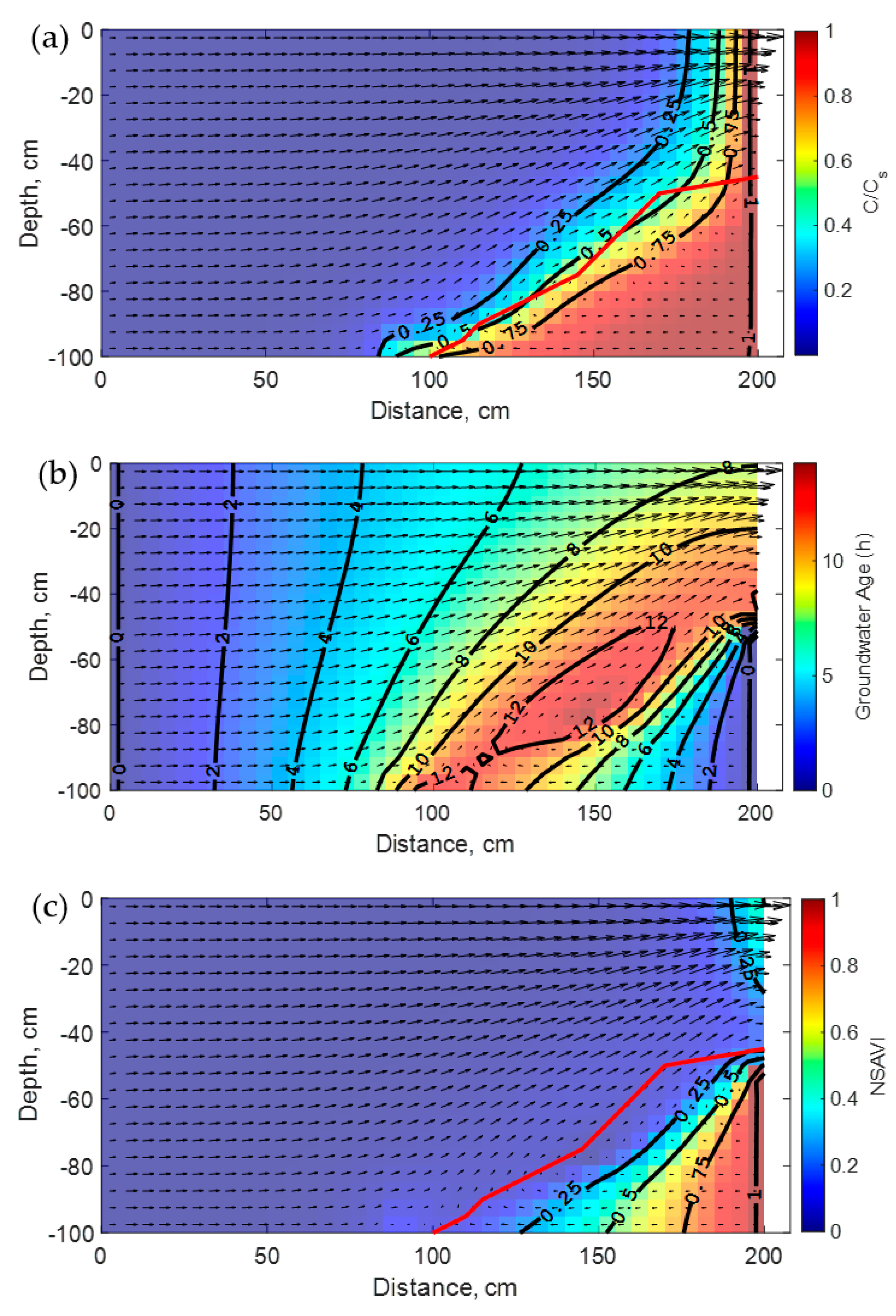
4.1.2. The Heterogeneous Diffusive Henry Problems
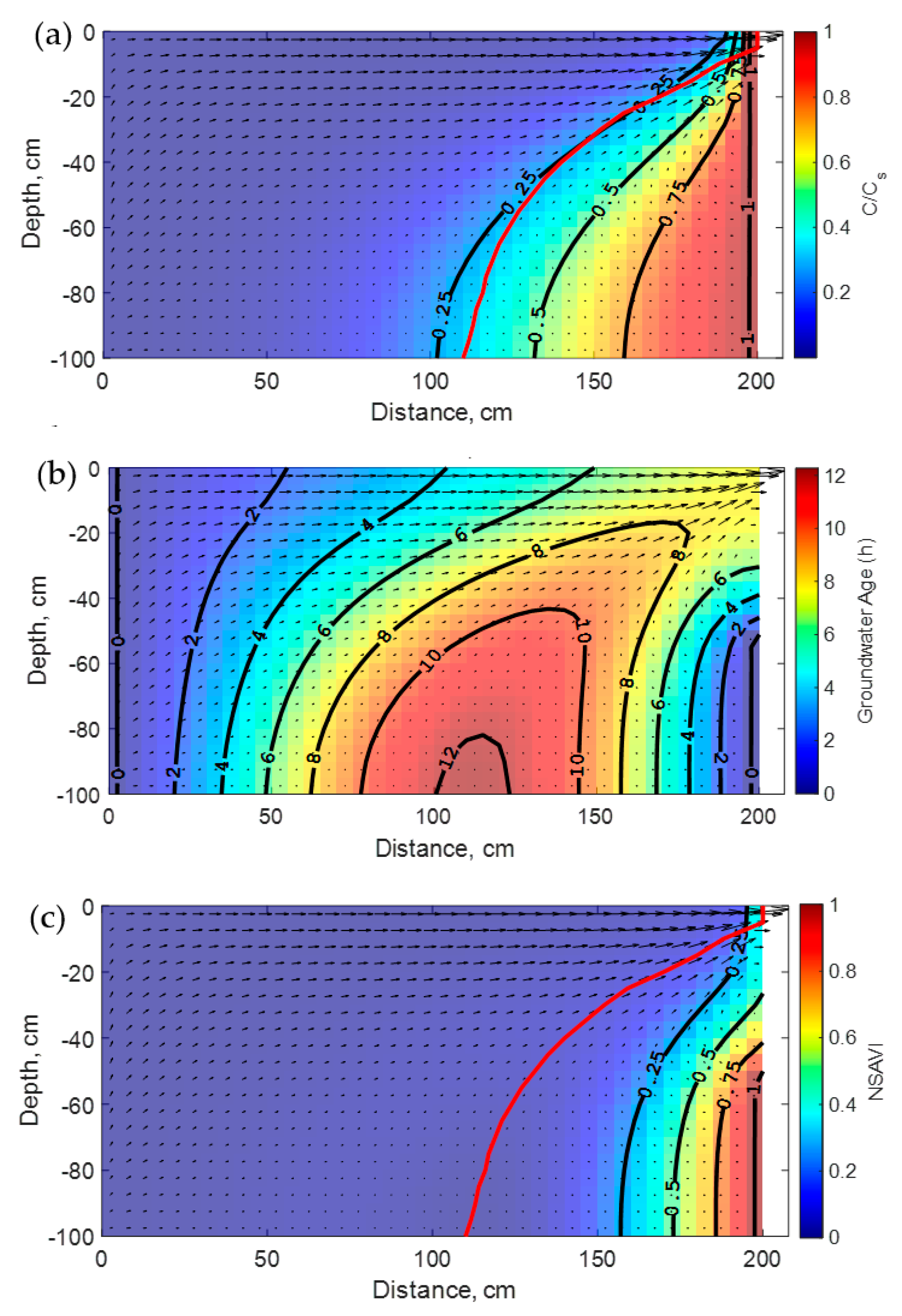
4.1.3. The Dispersive Henry Problems
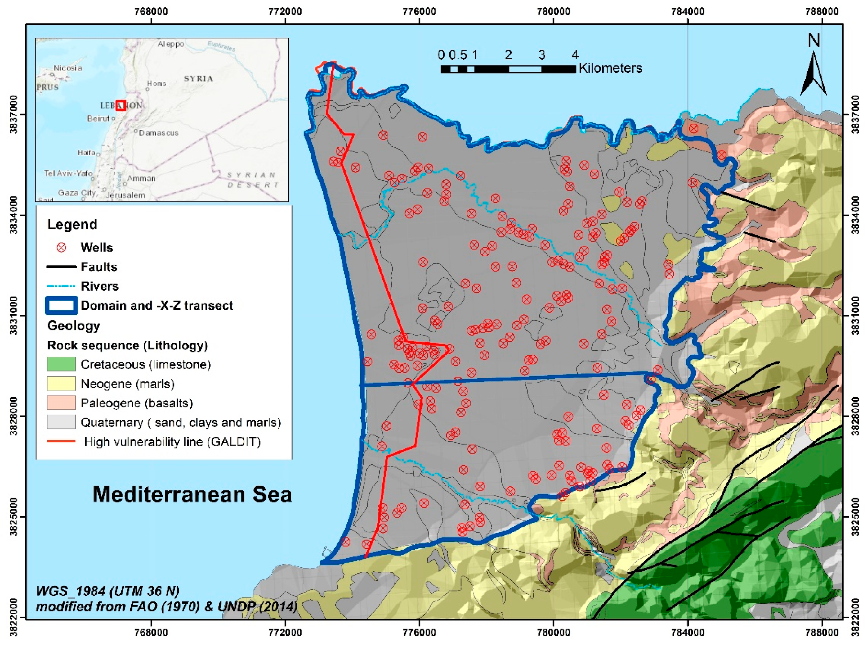
4.2. Example 2: The Akkar Coastal Aquifer (Lebanon)
5. Discussions
5.1. Implications of the Zero-Vulnerability Line/Surface on Coastal Aquifers Management
5.2. Implications for Optimal Management of Coastal Aquifers
5.3. Monitoring Network Design and Implementation
6. Conclusions
- The normalized saltwater vulnerability index was obtained from steady state distributions of the normalized concentration and a restriction of the mean groundwater age to a mean saltwater age distribution. The approach provides a novel way to shift from the concentration space into a vulnerability assessment space to evaluate the threats to coastal aquifers.
- The vulnerability to seawater intrusion is higher as the aquifer depth increases in homogeneous and heterogeneous stratified aquifers. This behavior is not reproducible when using the data-driven indexing methods giving further evidence of their conceptual limitations.
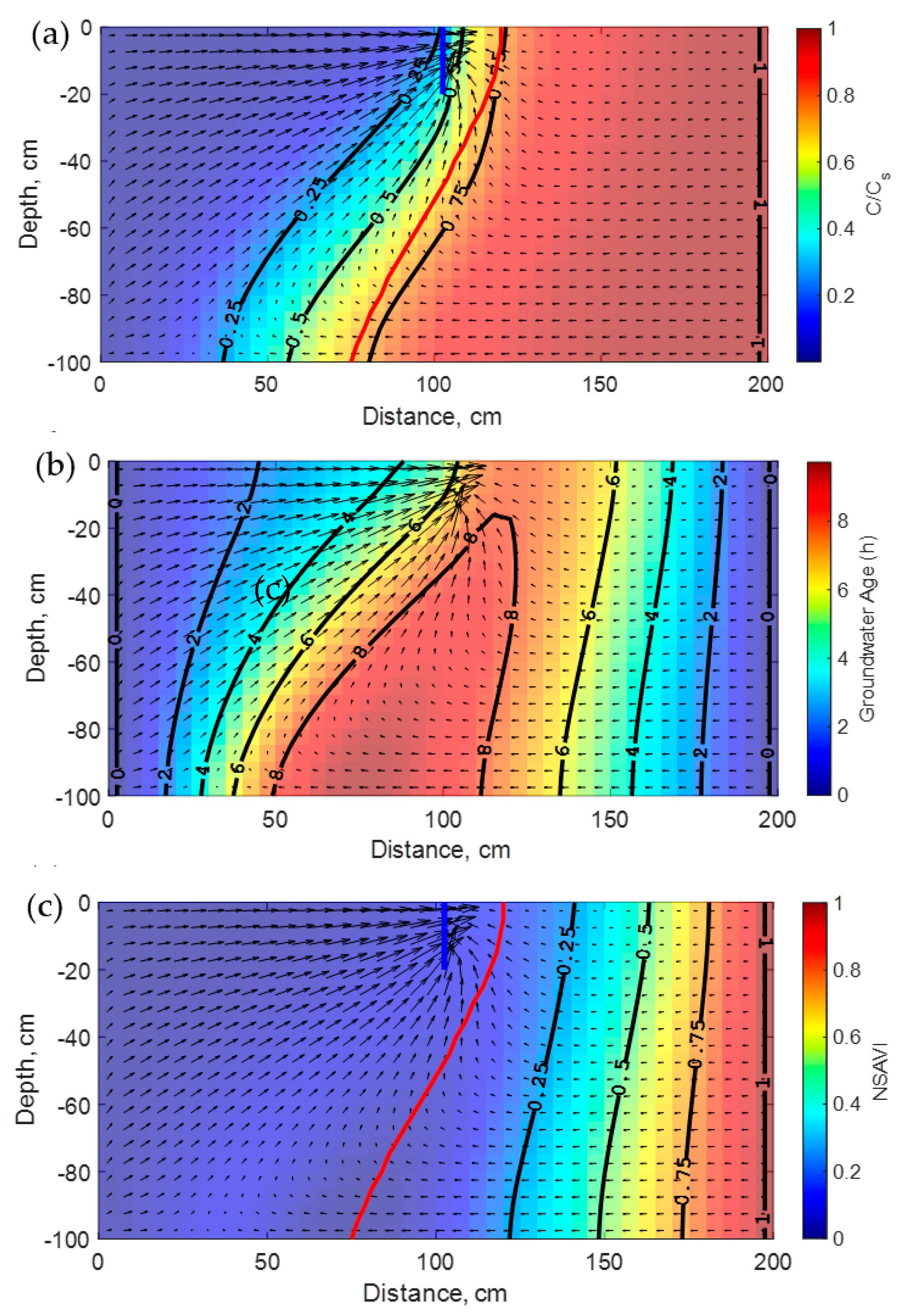
- The zero-vulnerability line/surface delineates the coastal area for which there is a probability of seawater intrusion to occur. This novel concept has important implications for the optimal management of coastal aquifers and establishing related risk assessment methodologies.
- The zero-vulnerability line position differs from that of the 50% isochlor. As the strength of anthropogenic processes increase, the ZVL fits with increasing isochlor levels. Hence, the 50% isochlor is not a suitable metric to evaluate the vulnerability of coastal aquifers to seawater intrusion.
- The provided theoretical and field case study problems demonstrate the suitability of this approach to rank, compare and validate different scenarios for coastal water resources management.
Author Contributions
Funding
Institutional Review Board Statement
Data Availability Statement
Acknowledgments
Conflicts of Interest
References
- Wetzelhuetter, C. Groundwater in the Coastal Zones of Asia-Pacific; Springer: Dordrecht, The Netherlands, 2015; pp. 317–342. [Google Scholar]
- United Nations Environment Programme. Marine and Coastal Ecosystems and Human Well-Being: A Synthesis Report Based on the Findings of the Millennium Ecosystem Assessment; UNEP: Nairobi, Kenya, 2006; 76p. [Google Scholar]
- Khan, M.R.; Koneshloo, M.; Knappett, P.S.K.; Ahmed, K.M.; Bostick, B.; Mailloux, B.J.; Mozumder, R.; Zahid, A.; Harvey, C.; Van Geen, A.; et al. Megacity pumping and preferential flow threaten groundwater quality. Nat. Commun. 2016, 7, 12833. [Google Scholar] [CrossRef] [PubMed]
- Tortella, B.D.; Tirado, D. Hotel water consumption at a seasonal mass tourist destination. The case of the island of Mallorca. J. Environ. Manag. 2011, 92, 2568–2579. [Google Scholar] [CrossRef] [PubMed]
- Kundzewicz, Z.; Döll, P. Will groundwater ease freshwater stress under climate change? Hydrol. Sci. J. 2009, 54, 665–675. [Google Scholar] [CrossRef] [Green Version]
- Ferguson, G.; Gleeson, T. Vulnerability of coastal aquifers to groundwater use and climate change. Nat. Clim. Chang. 2012, 2, 342–345. [Google Scholar] [CrossRef]
- Reilly, T.; Goodman, A. Analysis of saltwater upconing beneath a pumping well. J. Hydrol. 1987, 89, 169–204. [Google Scholar] [CrossRef]
- Zhou, Q.; Bear, J.; Bensabat, J. Saltwater Upconing and Decay Beneath a Well Pumping Above an Interface Zone. Transp. Porous Media 2005, 61, 337–363. [Google Scholar] [CrossRef]
- Rahman, M.A.; Hassan, K.M.; Alam, M.; Akid, A.S.M.; Riyad, A.S.M. Effects of salinity on land fertility in coastal areas of Bangladesh. Int. J. Renew. Energy Environ. Eng. 2014, 2, 174–179. [Google Scholar]
- Tully, K.L.; Weissman, D.; Wyner, W.J.; Miller, J.; Jordan, T. Soils in transition: Saltwater intrusion alters soil chemistry in agricultural fields. Biogeochemistry 2019, 142, 339–356. [Google Scholar] [CrossRef]
- Alam, M.Z.; Carpenter-Boggs, L.; Mitra, S.; Haque, M.; Halsey, J.; Rokonuzzaman, M.; Saha, B.; Moniruzzaman, M. Effect of Salinity Intrusion on Food Crops, Livestock, and Fish Species at Kalapara Coastal Belt in Bangladesh. J. Food Qual. 2017, 2017, 1–23. [Google Scholar] [CrossRef]
- Tuong, T.P.; Kam, S.P.; Hoanh, C.T.; Dung, L.C.; Khiem, N.T.; Barr, J.; Ben, D.C. Impact of seawater intrusion control on the environment, land use and household incomes in a coastal area. Paddy Water Environ. 2003, 1, 65–73. [Google Scholar] [CrossRef]
- Qahman, K.; Larabi, A. Evaluation and numerical modeling of seawater intrusion in the Gaza aquifer (Palestine). Hydrogeol. J. 2006, 14, 713–728. [Google Scholar] [CrossRef]
- Abd-Elhamid, H.F.; Javadi, A.A. A Cost-Effective Method to Control Seawater Intrusion in Coastal Aquifers. Water Resour. Manag. 2011, 25, 2755–2780. [Google Scholar] [CrossRef]
- Hussain, M.S.; Abd-Elhamid, H.F.; Javadi, A.A.; Sherif, M.M. Management of Seawater Intrusion in Coastal Aquifers: A Review. Water 2019, 11, 2467. [Google Scholar] [CrossRef] [Green Version]
- Werner, A.D.; Bakker, M.; Post, V.E.; Vandenbohede, A.; Lu, C.; Ataie-Ashtiani, B.; Simmons, C.T.; Barry, D. Seawater intrusion processes, investigation and management: Recent advances and future challenges. Adv. Water Resour. 2013, 51, 3–26. [Google Scholar] [CrossRef]
- Chachadi, A.G.; Lobo Ferreira, J.P. Sea water intrusion vulnerability mapping of aquifers using the GALDIT method. Coastin 2001, 4, 7–9. [Google Scholar]
- Chachadi, A.G.; Lobo Ferreira, J.P. Assessing aquifer vulnerability to sea-water intrusion using GALDIT method: Part 2, GALDIT indicators description. In Proceedings of the 4th Inter Celtic Colloquium on Hydrology and Management of Water Resources, Guimaraes, Portugal, 4–11 July 2005; Volume 310, pp. 172–180. [Google Scholar]
- Gorgij, A.D.; Moghaddam, A.A. Vulnerability Assessment of saltwater intrusion using simplified GAPDIT method: A case study of Azarshahr Plain Aquifer, East Azerbaijan, Iran. Arab. J. Geosci. 2016, 9, 1–13. [Google Scholar] [CrossRef]
- Sophiya, M.S.; Syed, T.H. Assessment of vulnerability to seawater intrusion and potential remediation measures for coastal aquifers: A case study from eastern India. Environ. Earth Sci. 2013, 70, 1197–1209. [Google Scholar] [CrossRef]
- Gontara, M.; Allouche, N.; Jmal, I.; Bouri, S. Sensitivity analysis for the GALDIT method based on the assessment of vulnerability to pollution in the northern Sfax coastal aquifer, Tunisia. Arab. J. Geosci. 2016, 9, 416. [Google Scholar] [CrossRef]
- Allouche, N.; Maanan, M.; Gontara, M.; Rollo, N.; Jmal, I.; Bouri, S. A global risk approach to assessing groundwater vulnerability. Environ. Model. Softw. 2017, 88, 168–182. [Google Scholar] [CrossRef]
- Kazakis, N.; Spiliotis, M.; Voudouris, K.; Pliakas, F.-K.; Papadopoulos, B. A fuzzy multicriteria categorization of the GALDIT method to assess seawater intrusion vulnerability of coastal aquifers. Sci. Total. Environ. 2018, 621, 524–534. [Google Scholar] [CrossRef]
- Parizi, E.; Hosseini, S.M.; Ataie-Ashtiani, B.; Simmons, C.T. Vulnerability mapping of coastal aquifers to seawater intrusion: Review, development and application. J. Hydrol. 2019, 570, 555–573. [Google Scholar] [CrossRef]
- Foster, S.S.D.; Hirata, R.; Andreo, B. The aquifer pollution vulnerability concept: Aid or impediment in promoting groundwater protection? Hydrogeol. J. 2013, 21, 1389–1392. [Google Scholar] [CrossRef]
- Werner, A.D.; Ward, J.; Morgan, L.; Simmons, C.T.; Robinson, N.I.; Teubner, M.D. Vulnerability Indicators of Sea Water Intrusion. Groundwater 2011, 50, 48–58. [Google Scholar] [CrossRef] [PubMed]
- Morgan, L.; Werner, A. Seawater intrusion vulnerability indicators for freshwater lenses in strip islands. J. Hydrol. 2014, 508, 322–327. [Google Scholar] [CrossRef]
- Bear, J.; Cheng, A.H.-D. Modeling Groundwater Flow and Contaminant Transport; Springer: Berlin/Heidelberg, Germany, 2010. [Google Scholar]
- Zheng, C.; Bennett, G.D. Applied Contaminant Transport Modeling, 2nd ed.; Wiley: New York, NY, USA, 2002. [Google Scholar]
- Huyakorn, P.S.; Pinder, G.F. The Computational Methods in Subsurface Flow; Elsevier BV: Amsterdam, The Netherlands, 1983. [Google Scholar]
- Margat, J. Vulnerability of Groundwater to Pollution: Database Mapping; BRGM Publication 68-SGL 198: Orléans, France, 1968. [Google Scholar]
- Vrba, J.; Zoporozec, A. (Eds.) Guidebook on Mapping Groundwater Vulnerability; International Contributions to Hydrology; H. Heise Publishing: Hannover, Germany, 1994. [Google Scholar]
- Strack, O.D.L. A single-potential solution for regional interface problems in coastal aquifers. Water Resour. Res. 1976, 12, 1165–1174. [Google Scholar] [CrossRef]
- Morgan, L.K.; Werner, A.D. A national inventory of seawater intrusion vulnerability for Australia. J. Hydrol. Reg. Stud. 2015, 4, 686–698. [Google Scholar] [CrossRef] [Green Version]
- Yu, X.; Michael, H.A. Mechanisms, configuration typology, and vulnerability of pumping-induced seawater intrusion in heterogeneous aquifers. Adv. Water Resour. 2019, 128, 117–128. [Google Scholar] [CrossRef]
- Fetter, C.W. Water resources management in coastal plain aquifers. In Water for the Human Environment: Proceedings of the First World Congress on Water Resources; Chow, V.T., Ed.; International Water Resources Association: Chicago, IL, USA, 1973; pp. 322–331. [Google Scholar]
- Werner, A. On the classification of seawater intrusion. J. Hydrol. 2017, 551, 619–631. [Google Scholar] [CrossRef]
- Ballesteros, B.J.; Morell, I.; García-Menéndez, O.; Renau-Pruñonosa, A. A Standardized Index for Assessing Seawater Intrusion in Coastal Aquifers: The SITE Index. Water Resour. Manag. 2016, 30, 4513–4527. [Google Scholar] [CrossRef] [Green Version]
- Fidelibus, M.D.; Pulido-Bosch, A. Groundwater Temperature as an Indicator of the Vulnerability of Karst Coastal Aquifers. Geosciences 2018, 9, 23. [Google Scholar] [CrossRef] [Green Version]
- Momejian, N.; Abou Najm, M.; Alameddine, I.; El-Fadel, M. Can groundwater vulnerability models assess seawater intrusion? Environ. Impact Assess. Rev. 2019, 75, 13–26. [Google Scholar] [CrossRef] [Green Version]
- Voss, C.I.; Souza, W.R. Variable density flow and solute transport simulation of regional aquifers containing a narrow freshwater-saltwater transition zone. Water Resour. Res. 1987, 23, 1851–1866. [Google Scholar] [CrossRef]
- Anderson, M.P.; Woessner, W.W.; Hunt, R.J. Applied Groundwater Modeling—Simulation of Flow and Advective Transport, 2nd ed.; Elsevier: London, UK, 2015. [Google Scholar]
- Fusco, F.; Allocca, V.; Coda, S.; Cusano, D.; Tufano, R.; De Vita, P. Quantitative Assessment of Specific Vulnerability to Nitrate Pollution of Shallow Alluvial Aquifers by Process-Based and Empirical Approaches. Water 2020, 12, 269. [Google Scholar] [CrossRef] [Green Version]
- Larabi, A.; De Smedt, F. Numerical solution of 3-D groundwater flow involving free boundaries by a fixed finite element method. J. Hydrol. 1997, 201, 161–182. [Google Scholar] [CrossRef]
- Sbai, M.A. Modelling Three-Dimensional Groundwater Flow and Transport by Hexahedral Finite Elements. Ph.D. Thesis, Free University of Brussels, Belgium, Brussels, 1999. [Google Scholar]
- Sbai, M.A.; Larabi, A.; De Smedt, F. Modelling saltwater intrusion by a 3-D sharp interface finite element model. WIT Trans. Ecol. Environ. 1998, 24. [Google Scholar] [CrossRef]
- Keating, E.; Zyvoloski, G. A Stable and Efficient Numerical Algorithm for Unconfined Aquifer Analysis. Groundwater 2009, 47, 569–579. [Google Scholar] [CrossRef]
- Ataie-Ashtiani, B.; Werner, A.D.; Simmons, C.T.; Morgan, L.K.; Lu, C. How important is the impact of land-surface inundation on seawater intrusion caused by sea-level rise? Hydrogeol. J. 2013, 21, 1673–1677. [Google Scholar] [CrossRef]
- Voss, C.I.; Provost, A. SUTRA: A Model for 2D or 3D Saturated-Unsaturated, Variable-Density Ground-Water Flow with Solute or Energy Transport; US Geological Survey: Reston, VA, USA, 2002; p. 291. [Google Scholar]
- Langevin, C.D.; Thorne, D.T.J.; Dausman, A.M.; Sukop, M.C.; Guo, W. SEAWAT Version 4: A Computer Program for Simulation of Multi-Species Solute and Heat Transport. In Techniques and Methods; US Geological Survey: Reston, VA, USA, 2008; p. 39. [Google Scholar]
- Diersch, H.-J.G. FEFLOW: Finite Element Modeling of Flow, Mass and Heat Transport in Porous and Fractured Media; Springer: Berlin, Germany, 2013. [Google Scholar]
- Goode, D. Direct Simulation of Groundwater Age. Water Resour. Res. 1996, 32, 289–296. [Google Scholar] [CrossRef]
- Kazemi, G.A.; Lehr, J.H.; Perrochet, P. Groundwater Age; Wiley-Interscience: Hoboken, NJ, USA, 2006. [Google Scholar]
- Campana, M.E. Generation of Ground-Water Age Distributions. Groundwater 1987, 25, 51–58. [Google Scholar] [CrossRef]
- Castro, M.C.; Goblet, P. Calculation of ground water ages—A comparative analysis. Groundwater 2005, 43, 368–380. [Google Scholar] [CrossRef]
- Sbai, M.A.; Larabi, A. On Solving Groundwater Flow and Transport Models with Algebraic Multigrid Preconditioning. Groundwater 2021, 59, 100–108. [Google Scholar] [CrossRef] [PubMed]
- Henry, H.R. Effects of dispersion on salt encroachment in coastal aquifers. In Sea Water in Coastal Aquifers; United States Geological Survey Paper, 1964; pp. 70–78. [Google Scholar]
- Ségol, G. Classic Groundwater Simulations: Proving and Improving Numerical Models; Prentice-Hall: Old Tappan, NJ, USA, 1994. [Google Scholar]
- Frind, E.O. Simulation of long-term transient density-dependent transport in groundwater. Adv. Water Resour. 1982, 5, 73–88. [Google Scholar] [CrossRef]
- Galeati, G.; Gambolati, G.; Neuman, S.P. Coupled and partially coupled Eulerian-Lagrangian Model of freshwater-seawater mixing. Water Resour. Res. 1992, 28, 149–165. [Google Scholar] [CrossRef]
- Croucher, A.E.; O’Sullivan, M.J. The Henry Problem for Saltwater Intrusion. Water Resour. Res. 1995, 31, 1809–1814. [Google Scholar] [CrossRef]
- Simpson, M.J.; Clement, T.P. Improving the worthiness of the Henry problem as a benchmark for density-dependent groundwater flow models. Water Resour. Res. 2004, 40, 01504. [Google Scholar] [CrossRef]
- Fahs, M.; Ataie-Ashtiani, B.; Younes, A.; Simmons, C.T.; Ackerer, P. The Henry problem: New semi-analytical solution for velocity-dependent dispersion. Water Resour. Res. 2016, 52, 7382–7407. [Google Scholar] [CrossRef]
- Post, V.E.; Vandenbohede, A.; Werner, A.; Maimun, A.D.; Teubner, M.D. Groundwater ages in coastal aquifers. Adv. Water Resour. 2013, 57, 1–11. [Google Scholar] [CrossRef]
- Younes, A.; Fahs, M. Extension of the Henry semi-analytical solution for saltwater intrusion in stratified domains. Comput. Geosci. 2015, 19, 1207–1217. [Google Scholar] [CrossRef]
- Abarca, E.; Carrera, J.; Sanchez-Vila, X.; Dentz, M. Anisotropic dispersive Henry problem. Adv. Water Resour. 2007, 30, 913–926. [Google Scholar] [CrossRef]
- Zidane, A.; Younes, A.; Huggenberger, P.; Zechner, E. The Henry semi analytical solution for saltwater intrusion with reduced dispersion. Water Resour. Res. 2012, 48, W06533. [Google Scholar] [CrossRef]
- FAO. Projet de Développement Hydro-Agricole: Etude Hydrogéologique de la Plaine d’Akkar; République Libanaise, Ministère des Ressources Hydriques et Électriques: Beyrouth, Liban, 1970. [Google Scholar]
- United Nations Development Programme. Assessment of Groundwater Resources of Lebanon; Ministry of Energy and Water: Beirut, Lebanon, 2014. [Google Scholar]
- Zaarour, T. Application of GALDIT Index in the Mediterranean Region to Assess Vulnerability to Seawater Intrusion. Master’s Thesis, Lund University, Lund, Sweden, 2017. [Google Scholar]
- Shi, L.; Jiao, J.J. Seawater intrusion and coastal aquifer management in China: A review. Environ. Earth Sci. 2014, 72, 2811–2819. [Google Scholar] [CrossRef]
- Sreekanth, J.; Datta, B. Review: Simulation-optimization models for the management and monitoring of coastal aquifers. Hydrogeol. J. 2015, 23, 1155–1166. [Google Scholar] [CrossRef]
- Cheng, A.H.-D.; Halhal, D.; Naji, A.; Ouazar, D. Pumping optimization in saltwater-intruded coastal aquifers. Water Resour. Res. 2000, 36, 2155–2165. [Google Scholar] [CrossRef] [Green Version]
- Park, C.-H.; Aral, M. Multi-objective optimization of pumping rates and well placement in coastal aquifers. J. Hydrol. 2004, 290, 80–99. [Google Scholar] [CrossRef]
- Qahman, K.; Larabi, A.; Ouazar, D.; Naji, A.; Cheng, A.H.-D. Optimal and sustainable extraction of groundwater in coastal aquifers. Stoch. Environ. Res. Risk Assess. 2005, 19, 99–110. [Google Scholar] [CrossRef]
- Bray, B.S.; Yeh, W.W.-G. Improving Seawater Barrier Operation with Simulation Optimization in Southern California. J. Water Resour. Plan. Manag. 2008, 134, 171–180. [Google Scholar] [CrossRef]
- Kourakos, G.; Mantoglou, A. Simulation and Multi-Objective Management of Coastal Aquifers in Semi-Arid Regions. Water Resour. Manag. 2011, 25, 1063–1074. [Google Scholar] [CrossRef]
- Kourakos, G.; Mantoglou, A. Pumping optimization of coastal aquifers based on evolutionary algorithms and surrogate modular neural network models. Adv. Water Resour. 2009, 32, 507–521. [Google Scholar] [CrossRef]
- Sreekanth, J.; Datta, B. Multi-objective management of saltwater intrusion in coastal aquifers using genetic programming and modular neural network based surrogate models. J. Hydrol. 2010, 393, 245–256. [Google Scholar] [CrossRef]
- Sreekanth, J.; Datta, B. Coupled simulation-optimization model for coastal aquifer management using genetic programming-based ensemble surrogate models and multiple-realization optimization. Water Resour. Res. 2011, 47, 04516. [Google Scholar] [CrossRef] [Green Version]
- Razavi, S.; Tolson, B.; Burn, D.H. Review of surrogate modeling in water resources. Water Resour. Res. 2012, 48, 07401. [Google Scholar] [CrossRef]
- Asher, M.J.; Croke, B.; Jakeman, A.; Peeters, L. A review of surrogate models and their application to groundwater modeling. Water Resour. Res. 2015, 51, 5957–5973. [Google Scholar] [CrossRef]
- Sbai, M.A. Well Rate and Placement for Optimal Groundwater Remediation Design with A Surrogate Model. Water 2019, 11, 2233. [Google Scholar] [CrossRef] [Green Version]
- Christelis, V.; Mantoglou, A. Pumping Optimization of Coastal Aquifers Using Seawater Intrusion Models of Variable-Fidelity and Evolutionary Algorithms. Water Resour. Manag. 2018, 33, 555–568. [Google Scholar] [CrossRef] [Green Version]
- Mantoglou, A.; Papantoniou, M. Optimal design of pumping networks in coastal aquifers using sharp interface models. J. Hydrol. 2008, 361, 52–63. [Google Scholar] [CrossRef]
- Langevin, C.D.; Panday, S.; Provost, A.M. Hydraulic-head formulation for density-dependent flow and transport. Groundwater 2020, 58, 349–362. [Google Scholar] [CrossRef] [PubMed]
- Oldenburg, C.M.; Pruess, K. Dispersive Transport Dynamics in a Strongly Coupled Groundwater-Brine Flow System. Water Resour. Res. 1995, 31, 289–302. [Google Scholar] [CrossRef]
- Saad, Y. Iterative Methods for Sparse Linear Systems, 2nd ed.; SIAM: Philadelphia, PA, USA, 2003. [Google Scholar]
- Lott, P.; Walker, H.; Woodward, C.; Yang, U. An accelerated Picard method for nonlinear systems related to variably saturated flow. Adv. Water Resour. 2012, 38, 92–101. [Google Scholar] [CrossRef]


| Parameter | Diffusive Henry Problem | Dispersive Henry Problem |
|---|---|---|
| Freshwater density (Kg·m−3) | 1000 | 1000 |
| Seawater density (Kg·m−3) | 1025 | 1025 |
| Seawater salinity (Kg·m−3) | 35 | 35 |
| Vertical hydraulic conductivity (m·s−1) | 0.01 | 0.01 |
| Anisotropy ratio ( | 1 | 0.66 |
| Effective porosity | 0.35 | 0.35 |
| Molecular diffusion of salt (m2·s−1) | 1.886 × 10⁻⁵ | 0 |
| Longitudinal dispersivity (m) | 0 | 0.1 |
| Transverse dispersivity (m) | 0 | 0.01 |
| Freshwater flux qf (m·s−1) | 3.3 × 10⁻⁵ | 3.3 × 10⁻⁵ |
| Parameter | Value |
|---|---|
| Freshwater density (Kg·m−3) | 1000 |
| Seawater density (Kg·m−3) | 1025 |
| Seawater salinity (Kg·m−3) | 35 |
| Dynamic viscosity (Pa.s) | 1.002 × 10⁻³ |
| Unit 1: 1.01 × 10⁻¹² | |
| Unit 2: 1.01 × 10⁻¹² | |
| Vertical permeability (m2) | Unit 3: 8.15 × 10⁻¹² |
| Unit 4: 5.09 × 10⁻¹³ | |
| Unit 5: 1.01 × 10⁻¹⁴ | |
| Unit 6: 3.05 × 10⁻¹³ | |
| Anisotropy ratio ( | 0.1 |
| Effective porosity | Units 2, 3, 4: 0.3 |
| Units 1, 5, 6: 0.2 | |
| Molecular diffusion of salt (m2·s−1) | 10−9 |
| Longitudinal dispersivity (m) | 50 |
| Transverse dispersivity (m) | 5 |
| Average recharge R (m·s−1) | 3.86 × 10⁻⁷ |
| Mountain-block recharge q (m·s−1) | 6.40 × 10⁻⁹ |
Publisher’s Note: MDPI stays neutral with regard to jurisdictional claims in published maps and institutional affiliations. |
© 2021 by the authors. Licensee MDPI, Basel, Switzerland. This article is an open access article distributed under the terms and conditions of the Creative Commons Attribution (CC BY) license (https://creativecommons.org/licenses/by/4.0/).
Share and Cite
Sbai, M.A.; Larabi, A.; Fahs, M.; Doummar, J. A New Normalized Groundwater Age-Based Index for Quantitative Evaluation of the Vulnerability to Seawater Intrusion in Coastal Aquifers: Implications for Management and Risk Assessments. Water 2021, 13, 2496. https://doi.org/10.3390/w13182496
Sbai MA, Larabi A, Fahs M, Doummar J. A New Normalized Groundwater Age-Based Index for Quantitative Evaluation of the Vulnerability to Seawater Intrusion in Coastal Aquifers: Implications for Management and Risk Assessments. Water. 2021; 13(18):2496. https://doi.org/10.3390/w13182496
Chicago/Turabian StyleSbai, Mohammed Adil, Abdelkader Larabi, Marwan Fahs, and Joanna Doummar. 2021. "A New Normalized Groundwater Age-Based Index for Quantitative Evaluation of the Vulnerability to Seawater Intrusion in Coastal Aquifers: Implications for Management and Risk Assessments" Water 13, no. 18: 2496. https://doi.org/10.3390/w13182496
APA StyleSbai, M. A., Larabi, A., Fahs, M., & Doummar, J. (2021). A New Normalized Groundwater Age-Based Index for Quantitative Evaluation of the Vulnerability to Seawater Intrusion in Coastal Aquifers: Implications for Management and Risk Assessments. Water, 13(18), 2496. https://doi.org/10.3390/w13182496