Mapping Interflow Potential and the Validation of Index-Overlay Weightings by Using Coupled Surface Water and Groundwater Flow Model

Abstract

Interflow is an important water source contributing to river flow. It directly influences the near-surface water cycles for water resource management. This study focuses on assessing the interflow potential and quantifying the interflow in the downstream area along the Kaoping River in southern Taiwan. The interflow potential is first determined based on the modified index-overlay model, which employs the analytical hierarchy process (AHP) to calculate the ratings and weightings of the selected factors. The groundwater and surface water flow (GSFLOW) numerical model is then used to link the index-overlay model to quantify the interflow potential for practical applications. This study uses the Monte Carlo simulations to assess the influence of rainfall-induced variations on the interflow uncertainty in the study area. Results show that the high potential interflow zones are located in the high to middle elevation regions along the Kaoping River. Numerical simulations of the GSFLOW model show an interflow variation pattern that is similar to the interflow potential results obtained from the index-overlay model. The average interflow rates are approximately 3.5 × 10⁴ (m³/d) in the high elevation zones and 2.0 × 10⁴ (m³/d) near the coastal zones. The rainfall uncertainty strongly influences interflow rates in the wet seasons, especially the peaks of the storms or heavy rainfall events. Interflow rates are relatively stable in the dry seasons, indicating that interflow is a reliable water resource in the study area.

1. Introduction

In hydrology, interflow is the lateral movement of water in the unsaturated zone. It can return to the surface or enter a stream before becoming groundwater. Interflow is also the water flow zone in a porous media right below river beds, and the interflow is the interface for the interactions between surface water and groundwater. Interflow occurs when water infiltrates into the subsurface. When hydraulic conductivity decreases with depth, lateral flow proceeds downslope. It may exfiltrate as return flows, becoming overland flow. Such interface is important to the bioenvironmental system near the rivers. Exchange of water across the interface can result from local and upstream to downstream water movement in and out of the river beds and banks. Water exchange across the surface water–groundwater interface has been explored in some detail in the past few decades, with most studies focused on rivers, and it is increasingly studied concerning the effects on the chemical composition of surface and subsurface water and the distribution of biota [1,2,3,4]. In many arid and semiarid areas, interflow also plays an essential role in water resource management in dry seasons when the water levels in rivers are relatively low [5,6,7]. With varied climate conditions, high river discharge variations in dry and wet seasons are generally observed. Therefore, the assessment of available water resources from interflow has become a key process to support land-use planning and regional development. This available water resource from interflow can be considered as the interflow potential for specific reaches of rivers.

The concept of index-overlay models to create different types of potential or vulnerability maps has been widely used for many implementations. Such potential or vulnerability maps are critical references to decision-making for land-use planning, groundwater management, monitoring, and remediation [8,9,10,11]. Previous investigations have shown that the advantages of the index-overlay models are their ease of use, minimal data demand, and precise definition of parameters for site-specific problems. With the recent advances in Geographical Information Systems (GISs), index-overlay models are especially helpful for creating various types of potential maps in the fields of groundwater resource potential [12,13,14]. A GIS associated with useful tools enables the overlay and integration of multiple maps, representing the selected parameters to account for the groundwater potential [15,16,17]. The development of interflow potential maps can follow the same concept as groundwater potential. In an interflow potential map, the value of the potential represents the relative availability of interflow in river segments.

The interflow potential maps are fundamental for assessing groundwater and surface water interaction in a local water cycle. For most practical problems, developing interflow potential maps is efficient because the intrinsic parameters such as the river slope, river stage, river bed material, and the groundwater level near the river are usually the available hydrogeological data from the specific sites [18,19]. Users determine the weightings and ratings of different selected parameters. The summation of the weightings and ratings then creates the relative potential for a site-specific problem [20,21,22]. It is essential to validate the developed potential maps for practical cases. However, the validation of the interflow potential might require interflow observations, and the direct observations are usually limited. In many studies, the observations of interflow are based on the calculation of water balance in different reaches of the rivers [23,24,25]. The river discharge values across different river sections must account for the discharge differences of interflow, specifically between two river sections. The net interflow rates in different river sections are then the basis to validate the interflow potential map. River bed infiltration tests could show direct measurements of water flow in and out of the river bed [26,27,28,29]. However, the relatively small scale of the infiltration tests might not represent well the interflow dynamics at the target site. The question of how to upscale and integrate different types of observations is challenging because it is necessary to validate the interflow potential obtained from index-overlay models. A physical-based model that could reproduce the surface water and groundwater dynamics might be useful to solve this challenge. Previous studies such as Grodzka-Łukaszewska et al. (2017) [30] or Diaz et al. (2020) [31] used different models to account for the interactions between surface water and groundwater. However, the interflow was not included in the conceptual model in their studies. The study aims to develop a workflow that uses the physical-based numerical model to validate the index-overlay model and quantify the interflow in the downstream area along the Kaoping River. The study uses the analytic hierarchy process (AHP) to modify the weightings and ratings in the index-overlay model [10,11]. The quantification of the interflow potential relies on the integrated GSFLOW model to account for groundwater and surface water interactions. The study developed a basin-scale of the modular groundwater flow (MODFLOW) model for the entire Pingtung Plain groundwater basin (PPGB). The results of the basin-scale model then provide head conditions for a refined sub-model in the downstream area along the Kaoping River. The refined model then uses the GSFLOW model to quantify the interaction between surface water and groundwater in the local area. With the available river and groundwater observations, the basin- and local-scale transient models are calibrated and validated based on the three-year observations from January 2015 to December 2017. The accuracy evaluations for the numerical models use different statistical parameters such as the coefficient of determination (R²), coefficient of correlation (RE), Nash-Sutcliffe efficiency coefficient (NSE), normalized root-mean-square errors (NRMSE), and percent bias (Pbias) [32,33,34,35]. The interflow from the GSFLOW model is then used to evaluate the accuracy of the interflow potential map obtained from the index-overlay model. The study also uses Monte Carlo simulations (MCS) to quantify the rainfall-induced uncertainty for the refined modeling area along the Kaoping River.

2. Materials and Methods

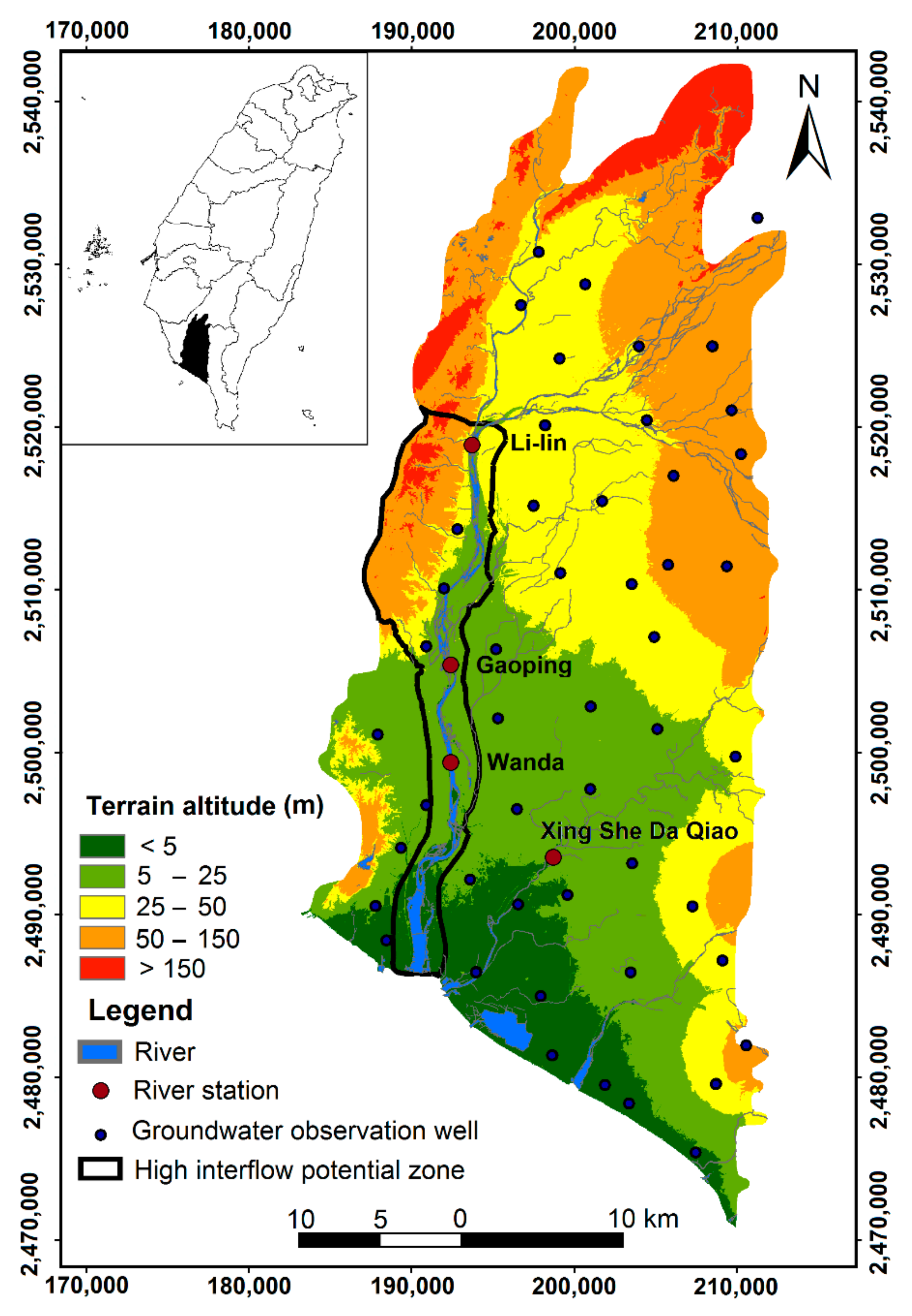
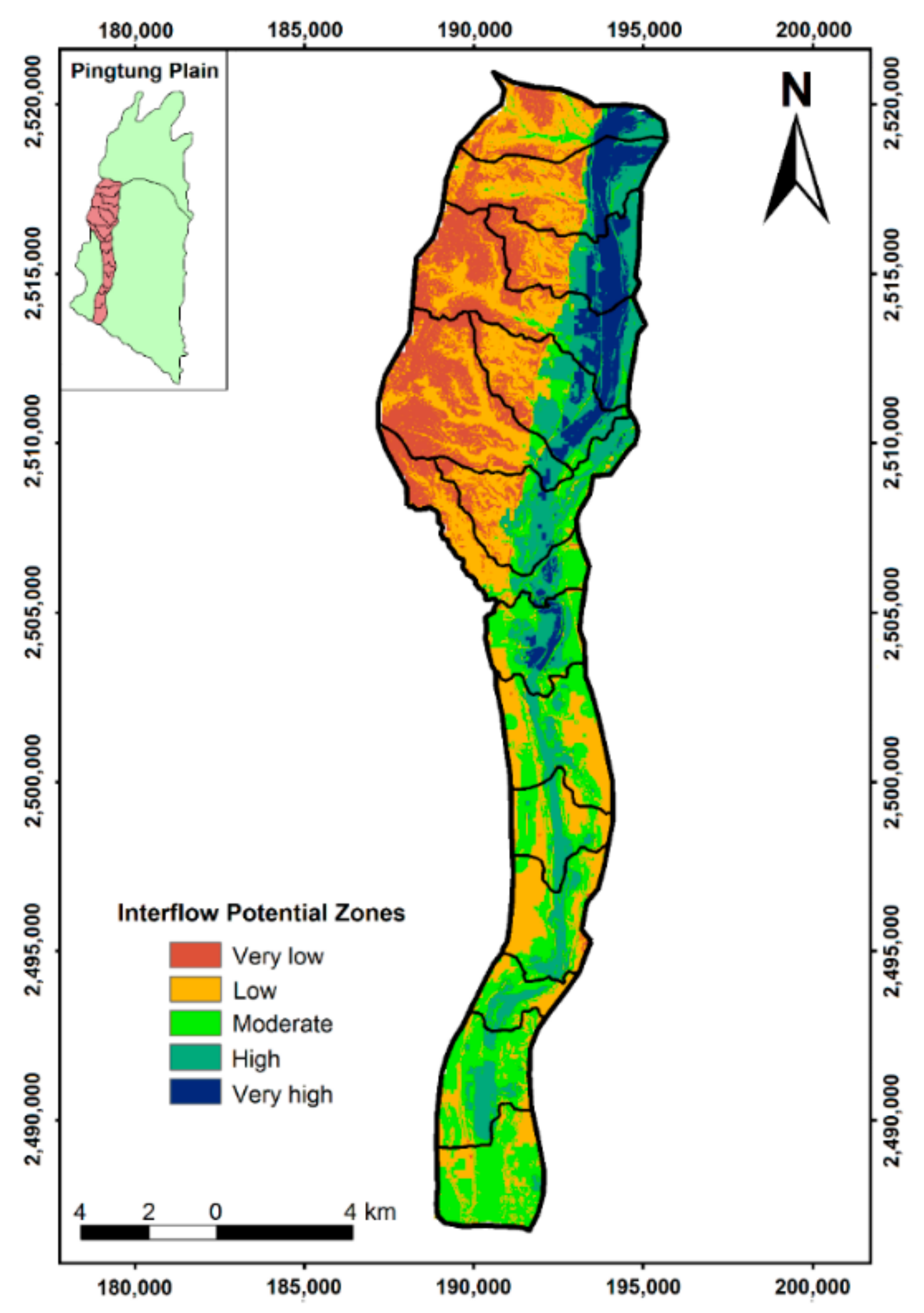
2.1. Study Area

The PPGB covers approximately 1300 km^2, and land surface elevation varies from the north to the south, located at Pingtung County in Taiwan (Figure 1). The annual precipitation in the PPGB varies significantly, from 1431 to 3597 mm, and the average precipitation is 2331 mm. Intense precipitation related to typhoons occurs three or four times per year on average [36]. Directions of major flow paths on the PPGB are similar to the terrain slope that is from the northeast to the southwest. In the PPGB, the Kaoping River is the largest river system, located in the south-west of the country, including part of the foothills in the west and flat plains in the south. Three tributaries contribute flow to the Kaoping River in its upper reaches, including the Laonung, Ailiao, and Qishan Creeks, and the discharge basins cover Kaohsiung City and Pingtung County. The upper and middle reaches of the Kaoping River originate from the high slopes of the mountainous area. The riverbed material is deposited in the middle and lower reaches, where the water flows through the mountainous zones into the delta plain. This sedimentation forms the main soil texture of the PPGB. These sediments are the primary materials distributed on the surface of the PPGB. In the PPGB, hydrogeological surveys have been conducted since 1995, and field hydraulic test data have been produced for the aquifer system [37]. The monitoring network was developed to monitor groundwater levels in different aquifer layers. To date, a total of 51 boreholes and 126 monitoring wells are available in the groundwater basin. The hydrogeological surveys showed that the sediment deposits in the downstream fan had formed four aquifer layers that are separated by low permeable marine sequences [37]. Field geological logs showed that there are no marine sequences observed in aquifers in the upstream fan area.

The study focuses on the downstream area of the Kaoping River, where considerable interflow potential has been recognized to support regional water resources (see the marked area in Figure 1) [38]. Figure 1 also shows the variations of the land surface in the PPGB. In the PPGB, there are foothills to the west and a relatively flat area near the Kaoping River. The high precipitation variations in the wet and dry seasons in the PPGB have made limited usage of surface water resources. Such difficulty leads to a challenging task in integrating available water resources for efficient and sustainable management. The downstream area along the Kaoping River (marked with a black polygon in Figure 1) has been recognized as the high interflow potential zone for regional water resources [39]. In this area, there are many interflow collection stations beside the river, and water collection pipes have been installed under the river to collect water for public use. Such public instruments support the alternative strategy to use the water resource from the river (i.e., the surface water), the groundwater, or both. The water collected from the porous media under the river is beneficial because of the relatively stable flow rate in dry seasons and high water quality in wet seasons.

2.2. Data Sources and Assumptions

The study aims to develop a workflow that uses a physically-based numerical model to validate an index-overlay model and quantify interflow in the downstream area along the Kaoping River. The basin-scale and local-scale numerical models comprise three years of simulations, particularly a calibration from January 2015 to December 2015 and a validation from January 2016 to December 2017. The steady-state model was calibrated based on the monthly averaged data in December 2014, which is a month earlier than the starting time of the transient simulations. In the refined sub-model along the downstream of the Kaoping River, there are three streamflow stations, namely Li-lin, Gaoping, and Wanda stations (see Figure 1). Because of the missing data at the Gaoping station, the calibration and validation processes mainly used the data from the Li-lin and Wanda stations. Based on the simulated GSFLOW results for the surface water and groundwater interactions, the volumetric interflow rates, such as one of the relative flows, are determined. In the GSFLOW model, the simulations rely on the predefined hydrologic response units (HRUs). In the study, the basin-scale MODFLOW model was developed with conditions similar to previous work in Tran et al. (2020) [40]. In this study, a sub-model was developed based on the specified heads obtained from the basin-scale MODFLOW model. In the sub-model, there are refined HRUs in the downstream area of the Kaoping River. Additional river discharge observations at the Wanda station were included in the sub-model. Based on the observations of groundwater levels and river discharge, calibration and validation of the GSFLOW model are required to represent the system response in the sub-model. In the study, the refined HRUs enabled the quantification of detailed interflow variation. Results could be used to assess the interflow potential maps created by the concept of index-overlay.

The study focuses on the high interflow potential zone. Interflow potential zones were assessed by the AHP technique that is used to modify the weightings and ratings of the selected factors in the index-overlay model. In the study, the selected factors in creating interflow potential maps are the land surface slope (S), transmissivity (T), the difference between river and groundwater levels (DH), depth to groundwater level (DG), and drainage density of the river system (DD). Specifically, the determination of the factors is based on the three-year averaged observations of the time-series observations in the study area. The slope map of the PPGB was derived from the digital elevation model (DEM) using the spatial analysis package in ArcGIS software. The DEM data were collected from the numerical terrain model of Taiwan, with a grid spacing of 20 m. Transmissivity describes the general ability of an aquifer to transmit water. The concept of transmissivity is similar to hydraulic conductivity, but the main difference is that transmissivity is a measurement that applies across the thickness of an aquifer. In the study, the transmissivity data were obtained from a report by the Taiwan Central Geological Survey [37].

The parameter DH represents the differences between river stages and groundwater levels along the river. DH indicates that the available water volume near the river channel controls the local interactions between groundwater and surface water. In addition, the water resource from interflow relies on the available water to be used for the water supply. Therefore, a small discrepancy between groundwater levels and river stages might yield high scores in calculating the interflow potential. The factor of DG was calculated based on the groundwater levels obtained from the monitoring network in the PPGB. In the study, data related to river and groundwater levels were provided by the Water Resources Agency in Taiwan and other studies [41,42]. A lower DG value signifies that more water volume is available near the land surface. Drainage density (DD) defines the total drainage length in a unit area, and the value indicates the closeness of the spacing of channels. In the study area, there is no artificial lining for the streams and channels. Therefore, we have assumed that the stream beds connect well with the aquifer system. Higher DD values can lead to higher interactions between groundwater and surface water. The factor represents the degree of fluvial dissection and is influenced by the resistance to erosion, infiltration capacity, vegetation cover, surface roughness and runoff indices, and climatic condition [43]. The DD is an important indicator that provides a numerical measurement of landscape dissection and surface runoff potential. The DD has been computed by using the line density analysis tool in the software ArcGIS.

3. Index-Overlay and Numerical Models

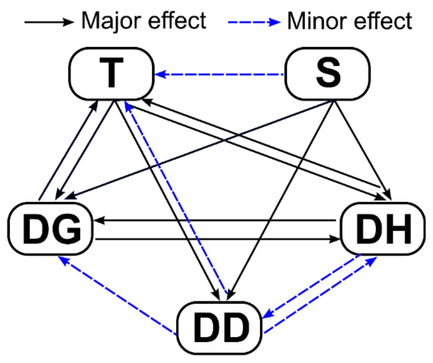
3.1. Index-Overlay Model

The present study considers multiple parameters for delineating the interflow potential map by using the Geographic Information System (GIS). The weightings for the potential map are determined based on the analytic hierarchy process (AHP) technique. In the study, the selected thematic parameters that influence interflow properties include the land surface slope (S), transmissivity (T), the difference between river and groundwater levels (DH), depth to groundwater level (DG), and drainage density of the river system (DD). These index parameters are represented with spatial distribution maps based on the weighted analysis of the AHP technique [44]. Each thematic factor in pairwise comparison is assessed for the relative rate by its influences on the interflow. All selected thematic factors were represented as raster data with a fixed pixel size of 20 × 20 m for all the map layers. The concept of the AHP is to break down the complex multicriteria problem into a hierarchy. It is based on the pairwise comparison of different criteria [45]. The pairwise comparison was then developed to identify the relative influence of a specific parameter on the interflow potential. The rescaled weightings were then determined based on the results from the numerical model.

In the study, the major and minor effects were assigned the scores of 1 and 0.5 following the concept proposed by previous studies (e.g., [20,21]). Note that judgment of the major and minor effects is based on the direct or indirect influence of the factors on the interflow potential. The influence between selected factors was also determined based on a similar concept. Figure 2 shows the influences of the selected thematic factors for generating the interflow potential map [20,21].

Table 1. Normalized pairwise matrix analysis for geometric mean calculation of selected parameters.

Factor	S	T	DH	DG	DD	Scale Weight	Geometric Mean
S	1.00	1.17	1.40	1.75	2.33	3.5	1.46
T	0.86	1.00	1.20	1.50	2.00	3.0	1.25
DH	0.71	0.83	1.00	1.25	1.67	2.5	1.04
DG	0.57	0.67	0.80	1.00	1.33	2.0	0.84
DD	0.43	0.50	0.60	0.75	1.00	1.5	0.63

summarizes the relative ratings for the thematic factors. Among the proposed relative rating of the five selected thematic factors, slope and transmissivity factors have shown relatively high ratings to calculate the interflow potential. The difference between river and groundwater levels has a mild rating compared to the slope and the transmissivity. The depth to groundwater and the drainage density show less influence on the interflow potential ratings. The ratings associated with the weightings for the factors were then integrated to create the potential map.

Figure 3 shows the distribution of the selected factors for generating the interflow potential map. Figure 3a is the distribution of the slope for the downstream area of the Kaoping River. The slope is estimated as an important parameter that influences the interflow potential in the study area. In Figure 3a, the slope map clearly shows the relatively flat areas with the slope varies from 0° to 2° along the Kaoping River. In particular, the slope in the study area varies from 0° to 62°. The local high slope is mainly distributed in the hill zone on the western side along the Kaoping River. In the low slope areas, we also obtained low DH and DG values (see Figure 3c,d), which might show relatively large water volumes in the aquifer system. Such large water volumes near the river system could indicate the relatively high interaction between groundwater and surface water.

Figure 3b shows the distribution of the transmissivity interpolated based on the field hydraulic tests conducted by Taiwan Central Geological Survey (Taiwan CGS). The study employed the ordinary Kriging method to create the interpolated transmissivity map. In general, the transmissivity varies from upstream to downstream along the Kaoping River. Figure 3c,d shows the DH and DG maps based on a similar interpolation algorithm by considering three-year averaged groundwater levels and river stages. In the study, the defined cell size in the DEM has been used to calculate the drainage density. Figure 3e shows the drainage density for estimating the interflow potential map. We found that the slope of the river basin also influences the development of the drainage pattern. In the foothill zone, there are local high drainage density areas. However, the high and continuous drainage density areas are mainly near the main channel of the Kaoping River (see Figure 3e).

The data shown in Figure 3 are fundamental to create the interflow potential map. We further classified the data map into five different levels in the study, including very high, high, moderate, low, and very low. The determination of the thresholds depends on the specific characteristic of each selected factor.

Table 2. Assigned and normalized weights of feature classes for the selected parameters to calculate interflow potential.

Factors	Descriptive Level	Domain of Effect	Assigned Weight (AW)	Geometric Mean (G)	Normalized Weight N = (AW/G)
Slope (S)	Very high	0–2°	9	1.46	6.16
[degree]	High	2–5°	7		4.79
	Moderate	5–10°	5		3.42
	Low	10–20°	3		2.05
	Very low	>20°	1		0.68
Transmissivity (T)	Very high	2340–3040	7.5	1.25	5.99
[m2/d]	High	1840–2340	6		4.79
	Moderate	1480–1840	4		3.19
	Low	1040–1480	2.5		2.00
	Very low	500–1040	1		0.80
River-GW level	Very high	<0	6.5	1.04	6.23
difference (DH)	High	0–5	6		5.75
[m]	Moderate	5–10	5		4.79
	Low	10–15	1		0.96
	Very low	> 15	1		0.96
Depth to	Very high	< 0	5	0.84	5.99
groundwater (DG)	High	0–5	4		4.79
[m]	Moderate	5–15	3		3.59
	Low	15–100	2		2.39
	Very low	>100	1		1.20
Drainage density (DD)	Very high	0.005–0.015	4	0.63	6.39
[m/m2]	High	0.003–0.005	3		4.79
	Moderate	0.002–0.003	2		3.19
	Low	0.001–0.002	1.5		2.39
	Very low	0–0.001	1		1.60

lists the selected thematic factors and the determined weightings for the interflow potential. The weightings, which vary from 5 to 1, represent the five influenced levels. In the study, the assigned weights (AWs) refer to the fundamental scale of nine levels proposed by Satty (1980) [46]. Based on the normalized weightings, the interflow potential could be obtained by summing the products of the respective factors and weights. The equation for the calculation of the interflow potential (IP) has the following formula:

$${\mathrm{IP}=\mathrm{S}}_{\mathrm{r}}{\mathrm{S}}_{\mathrm{w}}{+\mathrm{T}}_{\mathrm{r}}{\mathrm{T}}_{\mathrm{w}}{+\mathrm{DH}}_{\mathrm{r}}{\mathrm{DH}}_{\mathrm{w}}{+\mathrm{DG}}_{\mathrm{r}}{\mathrm{DG}}_{\mathrm{w}}{+\mathrm{DD}}_{\mathrm{r}}{\mathrm{DD}}_{\mathrm{w}},$$

(1)

where S, T, DH, DH, DG, and DD represent the five hydrogeological parameters included in assessing interflow potential. Subscriptions r and w denote the corresponding ratings and weightings for the parameters. Note that the minimum and maximum values of the different factors are usually varying in different ranges. Therefore, the study used the normalized weights (Table 2) for the presentation. The advantage of normalization is to break down the relations of anomalies among different parameter maps.

3.2. GSFLOW Numerical Model

The GSFLOW model proposed by Markstrom et al. (2008) [47] is an integrated hydrological model that couples the Precipitation Runoff Modeling System (PRMS) with the Modular Groundwater Flow Model (MODFLOW). Specifically, the modeling framework in GSFLOW was divided into different conceptual regions, including the region between the plant canopy and the soil zone, the region of streams and lakes, and the region beneath the soil zone (i.e., under the water level). GSFLOW relies on PRMS to simulate the responses of the hydrologic processes in the regions between the plant canopy and the soil zone. Other regions require the solutions obtained from the MODFLOW model and the supporting packages. The rivers and lakes regions arecrucial for representing the interactions between surface water and groundwater. In the MODFLOW, the groundwater flow with the constant density can be described by the following formula [48]:

$$S\frac{\partial h}{\partial t}=\frac{\partial }{\partial x}(K_x\frac{\partial h}{\partial x})+\frac{\partial }{\partial y}(K_y\frac{\partial h}{\partial y})+\frac{\partial }{\partial z}(K_z\frac{\partial h}{\partial z})+W,$$

(2)

where $K_x$, $K_y$, $K_z$[LT⁻¹] are the hydraulic conductivity in the x-, y-, and z-directions, $h=h(x,y,z,t)$ [L] is the hydraulic head. $W=W(x,y,z,t)$[T⁻¹] is a volumetric flux per unit volume, representing the sources and sinks of an aquifer system. The parameter $S$ is the storage coefficient of the aquifer, and $t$ [T] is time. The solution to the above equation is based on a three-dimensional finite-difference scheme. Flow associated with external stresses (i.e., the W in Equation (2)), such as wells, areal recharge, evapotranspiration, drains, and rivers, can be simulated with steady and transient conditions.

In the present study, assessment of the interflow is focused on the downstream area of the Kaoping River. The challenging task is to quantify the interflow in a local area and consider the regional groundwater dynamics that might influence the local water budget. The concept of sub-model is therefore employed to account for the interflow in a local area. The study developed a basin-scale groundwater model (i.e., the MODFLOW model) and a sub-model that focused on the downstream area of the Kaoping River (see Figure 1 for details). The refined HRUs in the sub-model have been conducted by the GSFLOW model (see Figure 4). Figure 4a,b shows the conceptual models for the basin-scale model and the sub-model. The boundary conditions of the groundwater flow in the sub-model were assigned based on the head results obtained from the basin-scale MODFLOW model. Note that the basin-scale groundwater model is a transient state model with a fixed time step of one month. The sub-model was specified to use the MODFLOW transient head results and thus be consistent with the basin-scale model. In the sub-model, the GSFLOW model considered the time step of one day. The input data such as the precipitation and river discharge were used for observations and specified at a one-day time step. In the study, the groundwater flow based on the monthly time step was converted to the daily groundwater flow for the PRMS simulation. For practical use of the process, the groundwater flow is usually fixed in different months for the PRMS model. In the sub-model, the calibration and validation of the GSFLOW model relied on the observations of daily river discharge at the Li-lin and Wanda stations (please see Figure 1 for the locations).

The simulation of GSFLOW requires the definition of the HRUs for the simulation domain. Figure 4b shows the specified HRUs in the sub-model. We are interested in quantifying the interflow obtained from the GSFLOW model. The results were used to compare the interflow potential map developed using the AHP technique. The calculation of the interflow in GSFLOW uses the following mass balance formula:

$$I=f-ET-S_s-R,$$

(3)

where I [L³ T⁻¹] is the interflow and f [L³ T⁻¹] is the infiltration rate for a specific HRU. Variable ET [L³ T⁻¹] in Equation (3) is the evapotranspiration and S_s [L³ T⁻¹] represents the soil moisture storage. In the GSFLOW model, the moisture storage comprises the capillary, gravity, and preferential-flow reservoirs. The variable R [L³ T⁻¹] is the groundwater recharge. Note that the groundwater flow processes, such as areal recharge, leakage from streamflow to aquifers, groundwater discharge to streams, and groundwater pumping, were simulated using the MODFLOW model. The unsaturated zone flow (UZF) package in MODFLOW is required to simulate the infiltration through the unsaturated zone. The package, associated with the PRMS module, can adequately account for the complex water interactions between the land surface and unsaturated zones above the groundwater levels.

Precipitation is the most important parameter that influences the interflow. We have found that the precipitation in the PPGB varies significantly in wet and dry seasons. Based on the calibrated GSFLOW model in the sub-model, the study further conducted stochastic modeling to assess the interflow uncertainty induced by the precipitation variations in the PPGB. The stochastic modeling used the Monte Carlo simulation (MCS) approach. In the MCS, realizations of precipitation time series for three-year were generated and applied to the calibrated GSFLOW model in the sub-model. There are 100 realizations generated for the assessment of the uncertainty induced by the precipitation. Figure 5 shows an example of the precipitation realizations at a station for three years. Note that the precipitation observations from 2015 to 2017 are the basis to generate the precipitation time series. The study assumed that the observations of the precipitation time series are the mean precipitation at each rainfall station. Random fluctuations based on a fixed standard deviation (STD) of 21.14 (mm/d) in a Gaussian model are used to generate the precipitation fluctuations. In this study, the STD value represents an averaged fluctuations of precipitation time series collected from the rainfall station in the PPGB. The Gaussian distribution model is used to generate the fluctuations of the rainfall dataset. The fluctuation time-series of three-year length were then added back to the mean precipitation at different stations for the modeling. The generated precipitation data at stations were used with the Thiessen-weighted method to obtain daily precipitation in the simulation domain. The spatial and temporal variations of the precipitation might not be stationary conditions. It could be interesting to assess the effect of similar precipitation fluctuations on the interflow variations in the wet and dry seasons in the PPGB.

4. Results and Discussion

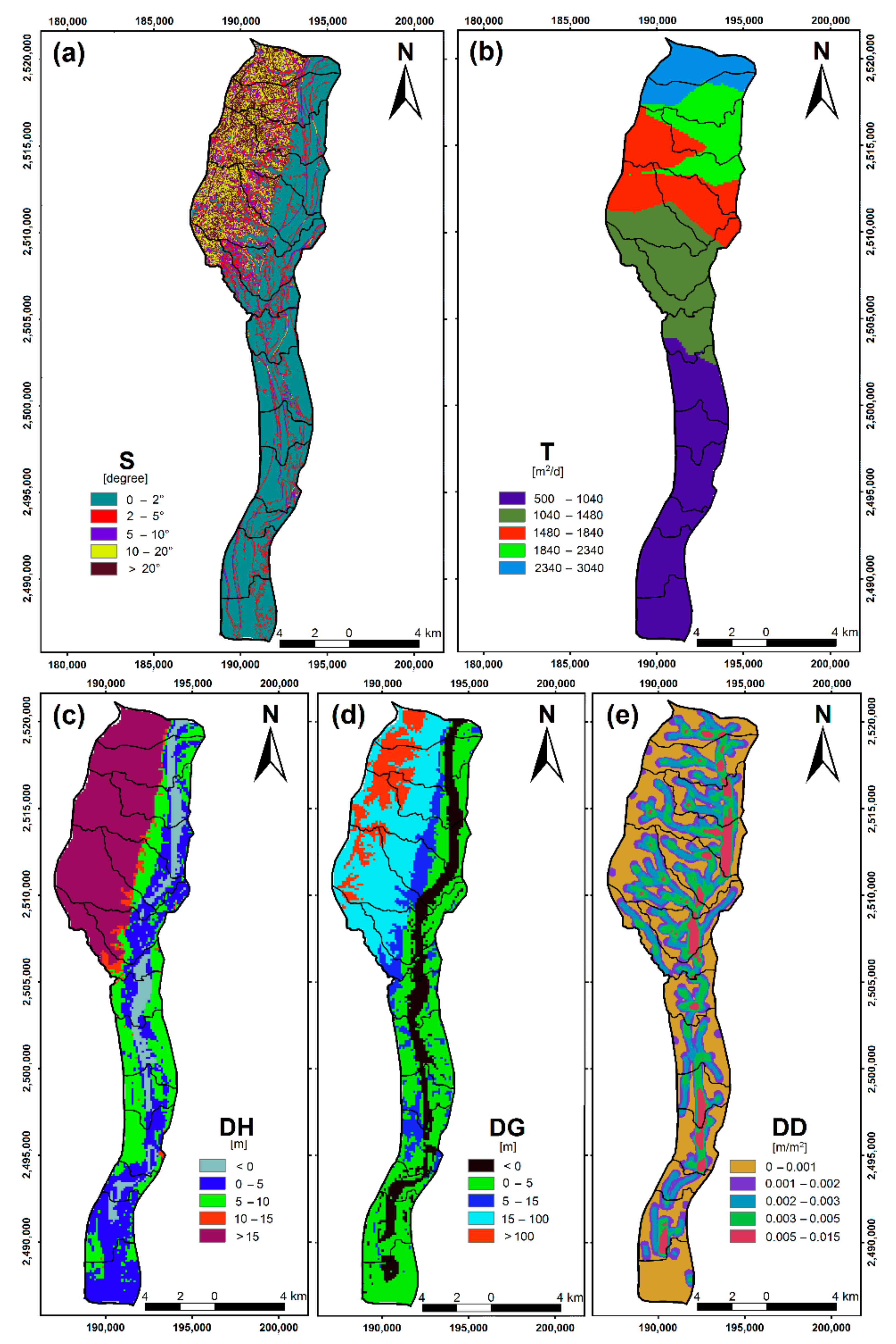
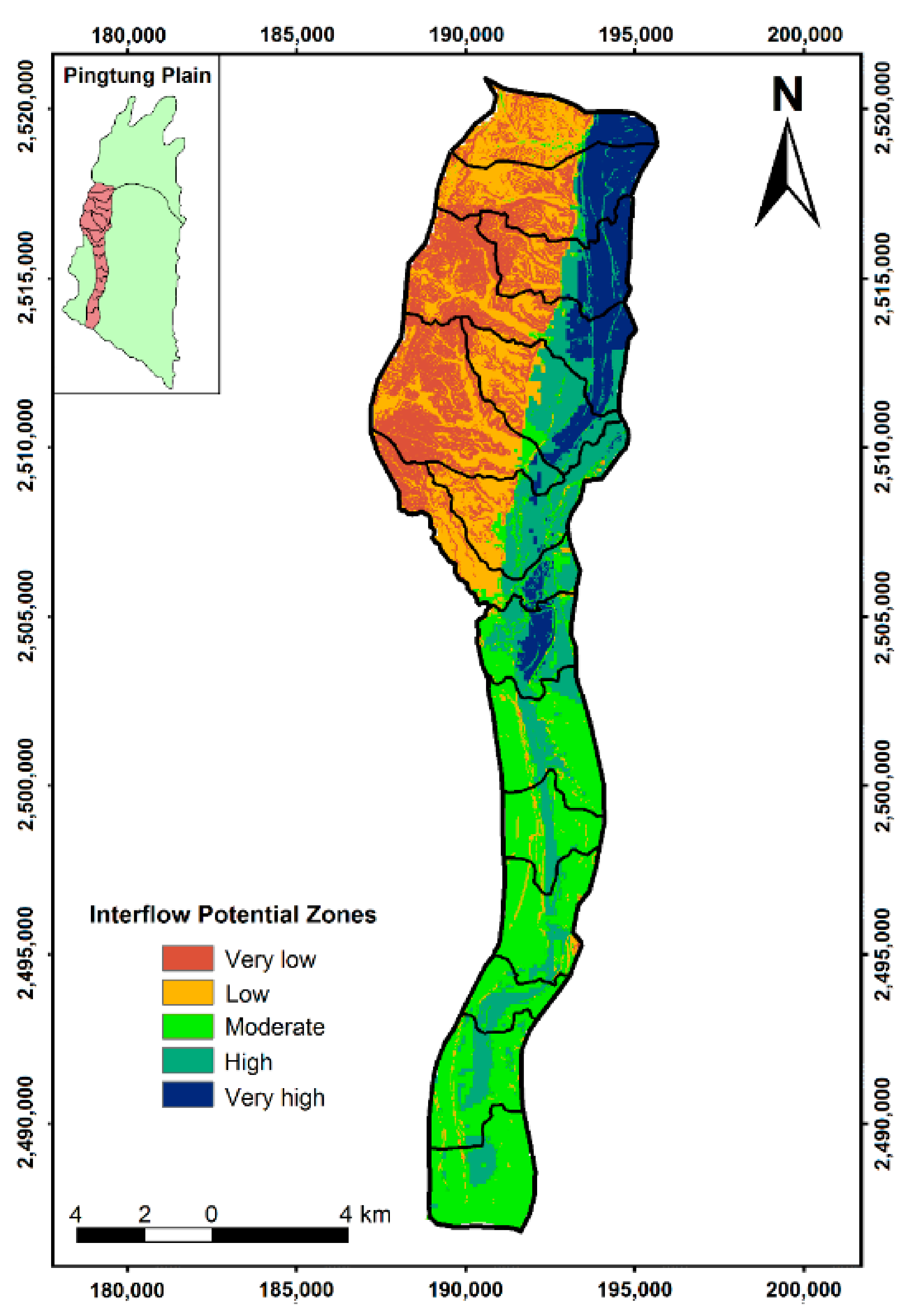
4.1. Interflow Potential Based on the Index-Overlay Model

The interflow potential zones were determined by the weighted overlay method. The weighted overlay techniques in the ArcGIS software have been integrated into the package of spatial analysis. Based on the available raster data and the ratings and weightings obtained from the AHP technique, Figure 6 shows the results of the interflow potential for the downstream area of the Kaoping River. The map clearly shows that the high interflow potential zones are mainly distributed along the Kaoping River, and the potential varies from upstream to downstream. We found that the very low and low levels of interflow potential are in the hill area and some flat areas away from the main channel of the Kaoping River. In the hill area, the index very low level dominates the area. However, there are low-level zones in the hill area. The patterns of the low-level zones are similar to the patterns of the drainage density (i.e., the DD parameter), indicating that DD has improved the interflow potential in the hill zone. Note that the transmissivity (T) might control the groundwater flow. There are no hydraulic test data in the hill zone in the study, and the T map in the hill zone relies on the interpolated T near the Kaoping River. Therefore, the interflow potential might be overestimated in the hill zone because the T might be relatively small in the hill zone.

In Figure 6, there is a clear interface between the hill zone and the river deposition zone in the north of the sub-model. This clear interface is consistent with the distribution of the parameters S, DH, and DG (see Figure 3). In this study, the values of inflow potential summarize the ratings and weightings obtained from the AHP technique. Slope has been recognized as the most influenced factor with the highest weighting to the interflow potential (Table 2). Low DH and DG values indicate a better connection between surface water and groundwater. To use the water resource, the large water volume near the land surface could facilitate the development of water supply systems. In summary, the interflow potential in Figure 6 has shown the availability of the near-surface water resource along the Kaoping River. However, the quantification of the interflow potential might require a physically-based model that accounts for the interaction between surface water and groundwater, and the physically-based GSFLOW model assists efficiently to validate the developed interflow potential map and quantify the interflow in the sub-model of Kaoping River.

4.2. Quantification of Interflow Potential Based on the GSFLOW Model

In this study, the proposed numerical model was developed through the calibration and validation procedures. These procedures used the data obtained from the hydrogeological monitoring network in the PPGB. The calibration procedure used the data in the year 2015. However, the validation considered the data obtained from 2016 to 2017. Note that the study applied the MODFLOW model for the entire PPGB, i.e., the basin-scale model. However, the GSFLOW was applied to the sub-model in the downstream area of the Kaoping River. The transient solutions of the basin-scale groundwater flow were then used for the flow boundaries in the sub-model. The results and discussion are based on the model outputs covering the simulation time from January 2015 to December 2017.

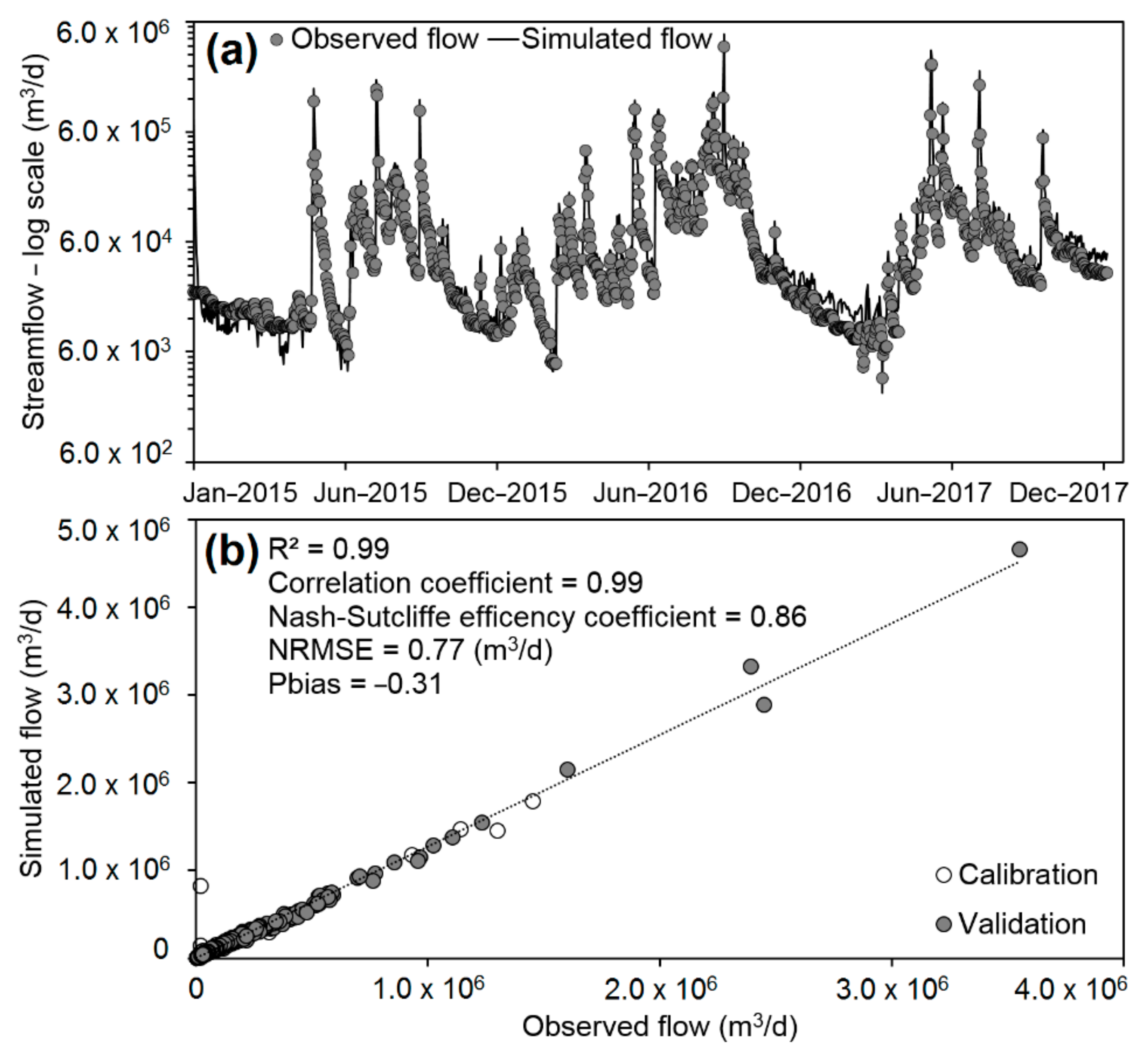
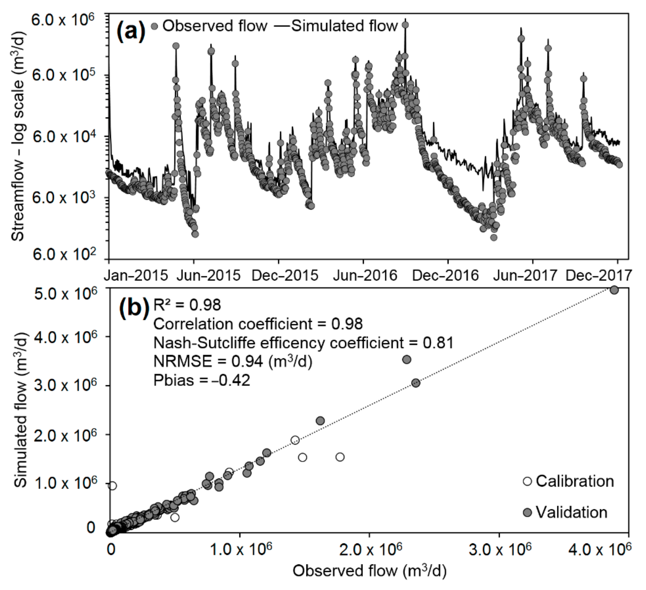
4.2.1. Model Calibration and Validation

The calibration and validation of the GSFLOW relied on the groundwater and surface water observations in the sub-model. In the sub-model, the Li-lin station is the upstream controlling point for the river discharge observations. The downstream river discharge observations are from the Wanda station (see Figure 1). In addition, the length of the Kaoping River in the sub-model is approximately 35 km from the Li-lin station to the Taiwan Strait. Based on these classified characteristics, the study area was divided into 15 HRUs (see Figure 4b) to estimate the detailed interflow dynamics.

Figure 7 and Figure 8 show the results of the simulated river discharge at two different stations. The data in 2015 were used for the calibration, and the data from 2016 to 2017 were used for the model validation. The GSFLOW results and the observations are consistent in the three years, indicating that the developed GSFLOW can reasonably reproduce the system dynamics of the surface water and groundwater interaction. The variations of the river discharge in wet and dry seasons have been accurately captured. In Figure 7a and Figure 8a, we found that the river discharge patterns at Li-lin and Wanda stations are similar. This is because of the relatively small drainage zones in the sub-model along the Kaoping River. Figure 7b and Figure 8b further show the direct comparison of the observed and the simulated results. We obtained high correlations between the observed and the simulated river discharge.

The determination (R²) values are 0.99 for the Li-lin station and 0.98 for the Wanda station. Using the Nash-Sutcliffe efficiency coefficient (NSE) to evaluate the simulation results, the results at the Li-lin station have better performances than those at the Wanda. The NSE values are 0.86 and 0.81 for the Li-lin and Wanda stations, respectively. However, the calculated normalized root-mean-square errors (NRMSE) performed differently for the two stations. The values of NRMSE are 0.77 (m³/d) for the Li-lin station and 0.94 (m³/d) for the Wanda station. The criterion to evaluate the accuracy of the simulation is the percent bias (Pbias) that aims to evaluate the average tendency of the observed and simulated results. In the study, the Pbias values for Li-lin and Wanda stations are −0.31 and −0.42 for the model validation, indicating that the tendency of the modeling results shows the overestimation of the observations at Li-lin and Wanda stations.

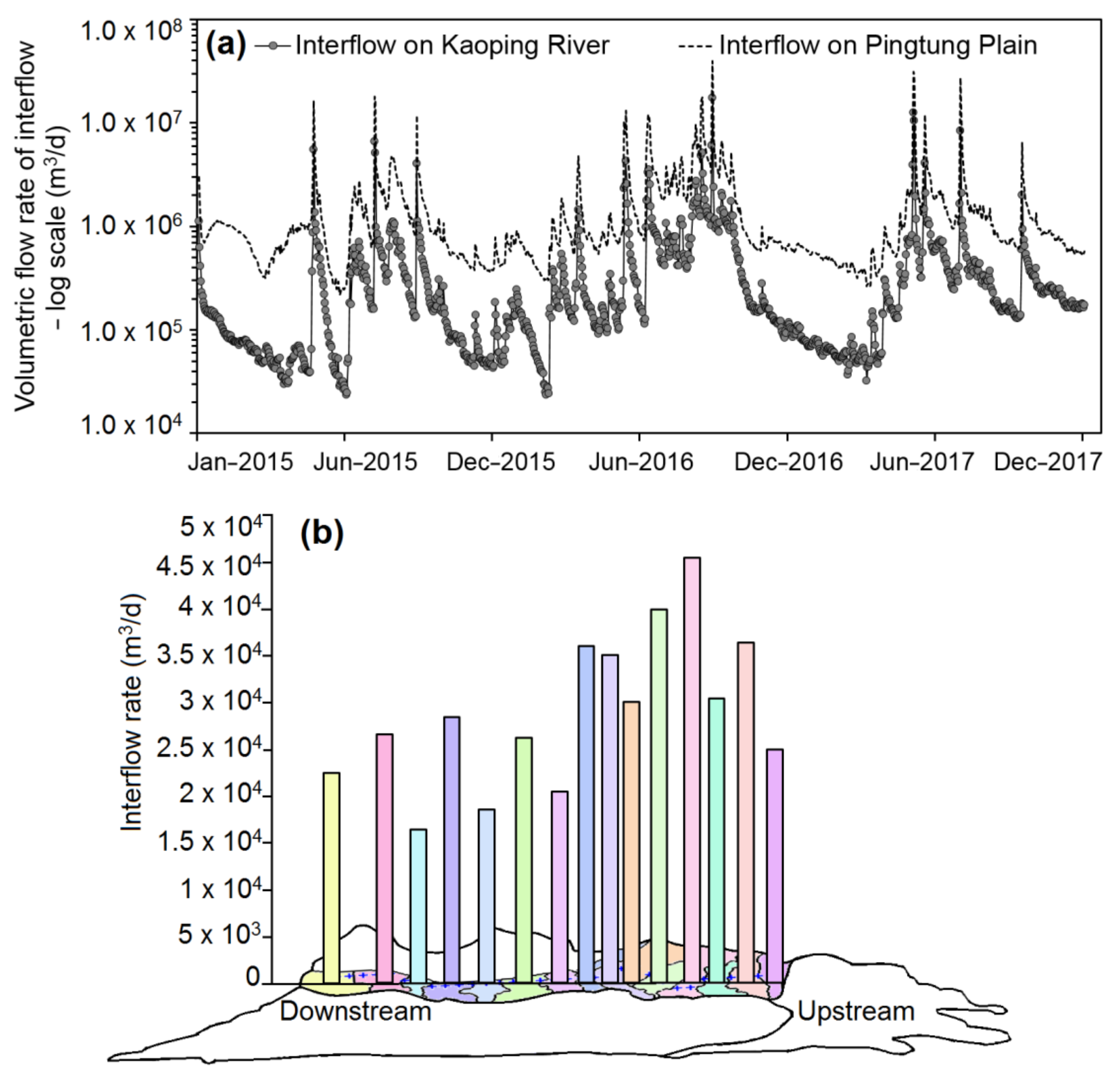
4.2.2. Interflow Dynamics in the Sub-Model

In the GSFLOW model, interflow is one of the flow components that account for the net flow contributing to the stream. The time-varied calculation of the interflow in each HRU relies on Equation (3), which considers the water cycle components near the interface between the surface water and groundwater. In addition to surface runoff, interflow is the important flow that supplies the flow to the stream. Figure 9a shows the temporal variations of the interflow in the sub-model and the entire PPGB. The results of the interflow for the entire PPGB were proposed by Tran et al. (2020). The relatively consistent rainfall influenced similar temporal variations of the interflow in the PPGB. In the sub-model, the interflow rates are approximately 1/10 of the interflow rates in the PPGB in the dry season. In general, we obtain high interflow rates in the wet seasons and low flow rates in the dry seasons. The interflow rates in the sub-model can vary within two different magnitudes, respectively in wet and dry seasons. In addition, the interflow rates in wet seasons in the sub-model show a similar amount of interflow rates that are obtained from the entire PPGB (see Figure 9a). The similar interflow magnitudes in the basin and local models represent the important role of the interflow potential in the downstream area of the Kaoping River. In the wet seasons, the interflow in the downstream area of the Kaoping River could be an important water resource because there is always high turbidity of the river water. The water treatments for public use have become a challenging task.

Figure 9b further shows the averaged interflow rates in different HRU along the Kaoping River. In the sub-model, the high interflow locations are generally distributed in the upstream area of the sub-model. These areas have relatively high altitude, steepness, and permeability properties. In the GSFLOW results, we found that the highest interflow rate is approximately 4.5 × 10⁴ (m³/d), corresponding to the volumetric flow per unit HRU area of 1.42 × 10⁻³ (m/d). Interflow decreases in the middle and middle-lower zones along the Kaoping River in the sub-model. The interflow rates near the coastal zone are slightly higher than those in the middle and middle-lower zones. In the sub-model, the lowest value of the interflow rate is about 1.5 × 10⁴ (m³/d), corresponding to 1.27 × 10⁻³ (m/d) of the volumetric flow per unit HRU area. However, the variations of the averaged interflow rates were insignificant in the HRUs along the Kaoping River.

We have obtained the interflow potential based on the index-overlay method and the associated AHP techniques to modify the ratings and weightings. Figure 9b could be a reference to evaluate the accuracy of the developed interflow potential map in Figure 6. The interflow potential map in Figure 6 had shown that the highest interflow potential is near the Li-lin station and the interflow potential gradually decreases along the Kaoping River to the downstream area. The lowest interflow potential zone is near the Wanda station. Figure 6 also shows a slightly lower interflow potential near the coastal zone as compared with that near the Wanda station. The results shown in Figure 6 are consistent with the distributions of the averaged interflow rates obtained from the GSFLOW simulation (see Figure 9b). To quantify the interflow potential based on the GSFLOW results, we have estimated the averaged interflow for different HRUs. In Figure 9b, the highest average interflow rate is approximately 3.5 × 10⁴ (m³/d) at high elevation zones in the sub-model. The value is 2.0 × 10⁴ (m³/d) near the coastal zones in the downstream Kaoping River. In this study, the developed interflow potential maps based on the selected factors can generally represent the physically-based numerical model, indicating that the selected thematic factors and the associated AHP ratings and weightings are acceptable.

It is worth discussing here the contribution of the selected factors to create the interflow potential map. Note that the interflow potential map has integrated the hydrogeological parameters to evaluate the relative potential for the study area. In this study, intrinsic parameters such as the slope (S) could significantly influence the behavior of T, DH, DG, and DD near the main channel of the river (see Figure 3c,d). It is recognized that all the factors might be influenced by other factors based on different geological processes and different temporal and spatial scales. For the value of T, it is clear that the surficial deposit near the river also depends on the surface slope. A higher slope would produce depositional sediments with relatively larger grain sizes, which lead to higher T values for the aquifer system. In the study, the distribution of T in the hill zone might not be accurate because of the limited T observations in the hill zone (see Figure 3b). The DH, DG, and DD are the indicators that show the available water volume near the land surface. The high slope areas in the hill zone might obtain high ratings and weightings. However, the available water volume is limited because of the high DH and DG values in the hill zone. A similar concept could be applied to the condition of the parameter DD. The limited water volume (i.e., high DH and DG values) in the hill zone gives a relatively low interflow potential in the hill zone. We found that the factor DD can play an important role in modifying the interflow potential map based on the AHP technique. Figure 10 presents the results of the interflow potential when the factor DD is excluded. The result without the DD factor in Figure 10 clearly shows the relatively high interflow potential upstream when compared to the map in Figure 6. Specifically, the result in Figure 6 also shows more detailed variations of the interflow potential near the main channel of the Kaoping River than the results shown in Figure 10.

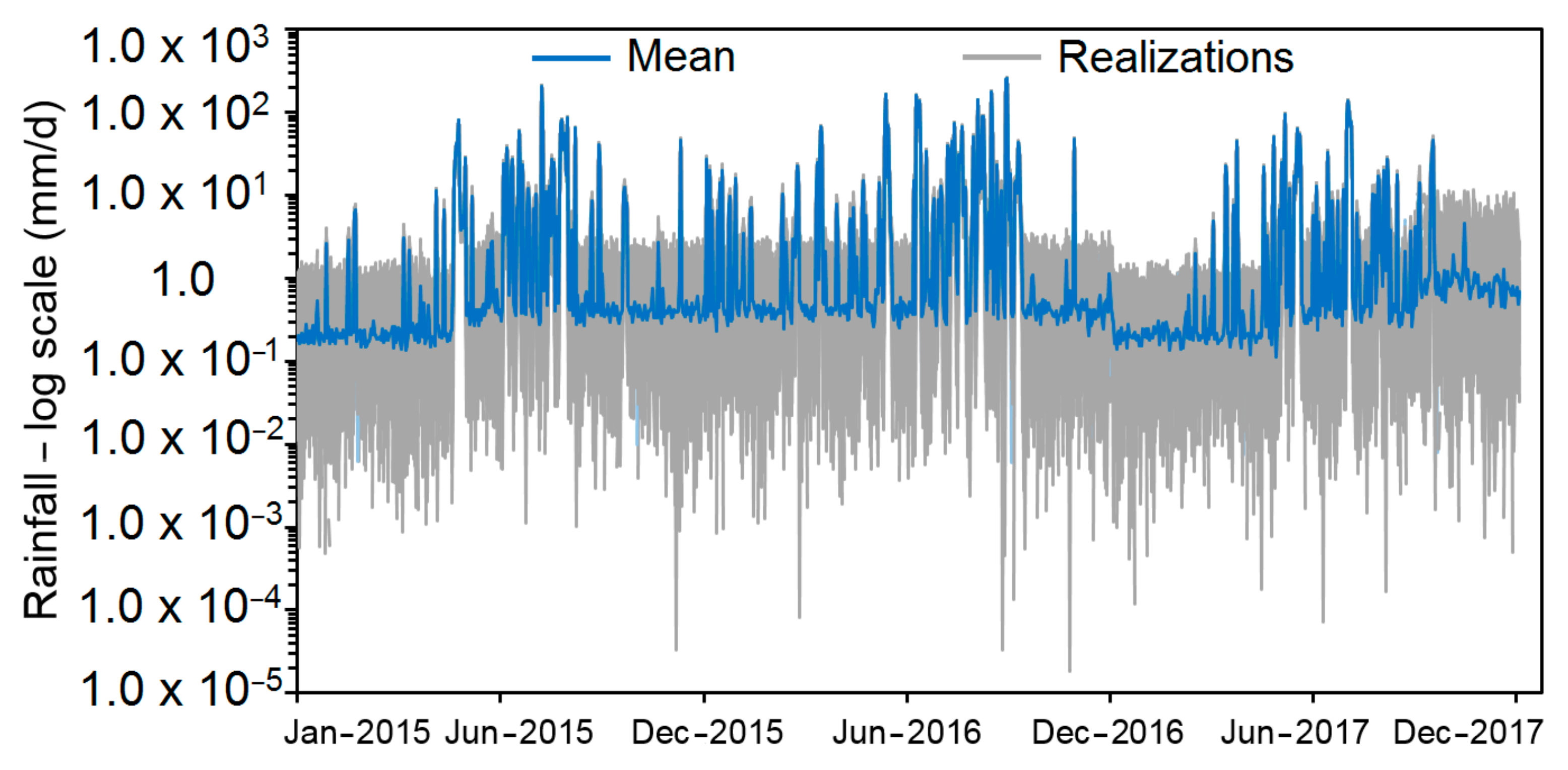
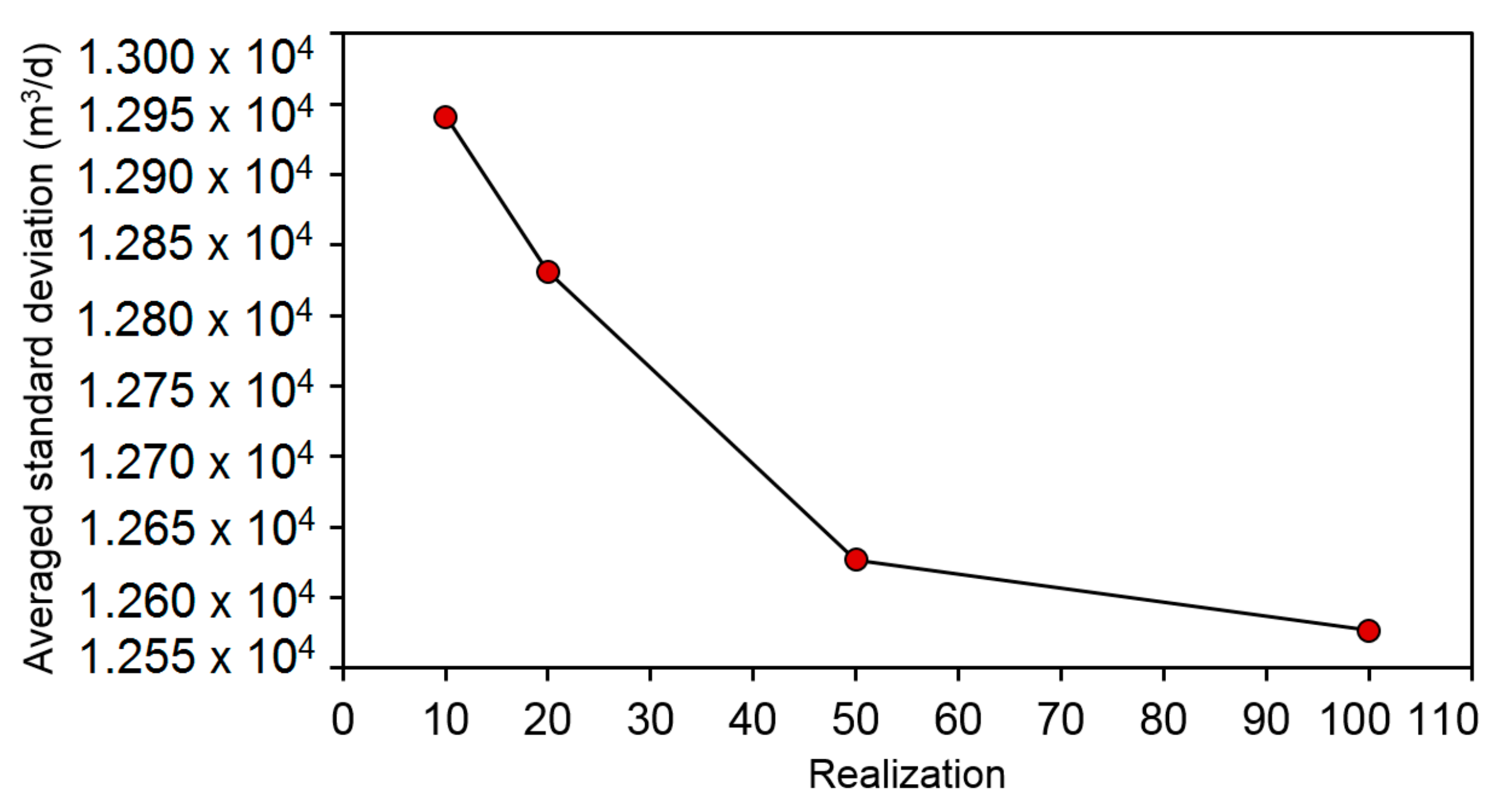
4.3. Interflow Uncertainty Induced by Precipitation

Based on the validated GSFLOW model, uncertainty analysis was conducted by using the concept of Monte Carlo simulations. One hundred realizations of precipitation time series were generated for the simulations (see Figure 5). In the study, we aim to quantify the influence of the input uncertainty (i.e., the precipitation) on the output uncertainty (i.e., the interflow). Figure 11 shows the variation of interflow STDs with the increased number of realizations. The result indicates a relatively small variation of the averaged STD for all the HRUs when the number of the realizations is greater than 50. Therefore, the 100 realizations in the Monte Carlo simulations could be representable to quantify the uncertainty of the interflow in the sub-model.

Figure 12 demonstrates the temporal variations of total interflow rates based on the precipitation realizations applied to the sub-model. Figure 12a shows the mean and realizations for the three-year simulations period. Figure 12b shows the variations of the mean and STD in a small period defined in Figure 12a (i.e., from December 2016 to April 2017) for demonstration purposes. In general, the variation of the precipitation in the PPGB has significantly influenced the variation of the interflow in the downstream area of the Kaoping River. With the high non-uniform precipitation in wet and dry seasons, the uncertainty of the interflow also varies significantly in wet and dry seasons. The uncertainty of the interflow is relatively higher in the wet seasons than that in the dry seasons. The result in Figure 12b has shown that a relatively stable variation of the interflow in the dry season from December 2016 to April 2017. The storm events such as those on December 6 to 8 and December 29 to 31 have clearly shown high variations based on the predefined mean precipitation in the model. Similar behavior is obtained in the wet seasons through the three-year simulations. However, the uncertainty is much higher in the storm events in the wet seasons. In this study, we previously calculated an STD of 21.14 (mm/d) for precipitation. Such mean variation of precipitation has produced the mean interflow STD of 1.26 × 10⁴ (m³/d), corresponding to STD of 1.42 × 10⁴ (m³/d) in the wet seasons and STD of 0.84 × 10⁴ (m³/d) in the dry seasons. The results show that the overall fluctuation of the interflow rate in the wet seasons is slightly higher than that in the dry seasons, indicating a relatively stable interflow rate in the study area. Note that we have determined the mean precipitation based on the results of the validated GSFLOW model. The variation pattern of the precipitation might be constrained by the original observations of the precipitation in the PPGB. Further implementation could use a design rainfall pattern for the mean precipitation in the model.

5. Conclusions

This study developed an index-overlay and a numerical model to assess the interflow potential and quantify the interflow in the downstream area along the Kaoping River in southern Taiwan. The analytical hierarchy process was used to modify the ratings and weightings for the interflow potential map. The GSFLOW numerical model was then employed to quantify the interflow potential for practical applications. The rainfall-induced uncertainty was assessed to characterize the critical water cycle components in the study area.

The results of the interflow potential show that the high interflow potential zones are mainly distributed along the Kaoping River, and the potential varies from the upstream to the downstream areas. The very low and low levels of interflow potential are in the hill area and some flat areas away from the main channel of the Kaoping River. The study obtained a clear interface of interflow potential between the hill zone and the river deposition zone in the study area. This clear interface is consistent with the distribution of the parameter S, DH, and DG, indicating the better connection between surface water and groundwater.

In the study, the calibration and validation of GSFLOW were based on 15 specified HRUs and were used to estimate the detailed interflow dynamics. The results of the simulated river discharge at two different stations are fitted well, indicating that the developed GSFLOW can reproduce the system dynamics of the surface water and groundwater interaction. In the sub-model, the interflow rates are approximately 1/10 of the interflow rates in the PPGB. In general, the interflow rates are high in the wet seasons and low in the dry seasons. The interflow rates in the model can vary within two orders of magnitudes. The high interflow locations are generally distributed in the upstream area and the interflow rate decreases in the middle and middle-lower zones along the Kaoping River. However, the variations of the averaged interflow rates were insignificant in the HRUs along the Kaoping River.

We have obtained the interflow potential based on the index-overlay model and the associated AHP techniques to modify the ratings and weightings. The interflow potential map shows consistently the distributions of the averaged interflow rates obtained from the GSFLOW simulation. The highest average interflow rate is approximately 3.5 × 10⁴ (m³/d) at high elevation zones, and the value is 2.0 × 10⁴ (m³/d) near the coastal zones in the downstream Kaoping River. The interflow potential maps developed based on the selected factors can reproduce well the physical-based numerical model, indicating that the selected thematic factors and the associated AHP ratings and weightings are acceptable. The factor DD can play an important role in modifying the interflow potential map based on the AHP technique.

The uncertainty analysis was conducted by using the Monte Carlo simulations. With 100 realizations of precipitation time series, the study quantifies the influence of precipitation uncertainty on interflow uncertainty. In general, the variation of the precipitation in the PPGB significantly influences the variation of interflow in the downstream area of the Kaoping River. The uncertainty of interflow is relatively higher in the wet season than in the dry season. The stochastic simulation obtained the averaged interflow STD of 1.89 × 10⁴ (m³/d) for the study area. From 2015 to 2017, the average STD was 2.35 × 10⁴ (m³/d) for the wet seasons, and the average STD was 1.42 × 10⁴ (m³/d) for the dry seasons. This is based on the calculated precipitation STD of 21.14 (mm/d). Such variation pattern of the precipitation might be constrained by the original observations of the precipitation in the PPGB. Further work could use a design rainfall pattern for the mean precipitation in the model.

References

1. Alley, W.M.; Healy, R.W.; LaBaugh, J.W.; Reilly, T.E. Flow and storage in groundwater systems. Science 2002, 296, 1985–1990. [Google Scholar] [CrossRef] [PubMed] [Green Version]
2. Dragon, K.; Marciniak, M. Chemical composition of groundwater and surface water in the Arctic environment (Petuniabukta region, central Spitsbergen). J. Hydrol. 2010, 386, 160–172. [Google Scholar] [CrossRef]
3. Barthel, R.; Banzhaf, S. Groundwater and Surface Water Interaction at the Regional-scale–A Review with Focus on Regional Integrated Models. Water Resour. Manag. 2016, 30, 1–32. [Google Scholar] [CrossRef] [Green Version]
4. Vasconcelos, V.V. What maintains the waters flowing in our rivers? Appl. Water Sci. 2017, 7, 1579–1593. [Google Scholar] [CrossRef] [Green Version]
5. Huntington, J.L.; Niswonger, R.G. Role of surface-water and groundwater interactions on projected summertime streamflow in snow dominated regions: An integrated modeling approach. Water Resour. Res. 2012, 48, 1–20. [Google Scholar] [CrossRef] [Green Version]
6. Zhang, Z.; Chen, X.; Xu, C.Y.; Hong, Y.; Hardy, J.; Sun, Z. Examining the influence of river-lake interaction on the drought and water resources in the Poyang Lake basin. J. Hydrol. 2015, 522, 510–521. [Google Scholar] [CrossRef]
7. Carroll, R.W.H.; Deems, J.S.; Niswonger, R.; Schumer, R.; Williams, K.H. The Importance of Interflow to Groundwater Recharge in a Snowmelt-Dominated Headwater Basin. Geophys. Res. Lett. 2019, 46, 5899–5908. [Google Scholar] [CrossRef] [Green Version]
8. Demiroǧlu, M.; Dowd, J. The utility of vulnerability maps and GIS in groundwater management: A case study. Turkish J. Earth Sci. 2014, 23, 80–90. [Google Scholar] [CrossRef]
9. Jang, W.S.; Engel, B.; Harbor, J.; Theller, L. Aquifer vulnerability assessment for sustainable groundwater management using DRASTIC. Water 2017, 9, 792. [Google Scholar] [CrossRef] [Green Version]
10. Vu, T.D.; Ni, C.F.; Li, W.C.; Truong, M.H. Modified index-overlay method to assess spatial-temporal variations of groundwater vulnerability and groundwater contamination risk in areas with variable activities of agriculture developments. Water 2019, 11, 2492. [Google Scholar] [CrossRef] [Green Version]
11. Vu, T.D.; Ni, C.F.; Li, W.C.; Truong, M.H.; Hsu, S.M. Predictions of groundwater vulnerability and sustainability by an integrated index-overlay method and physical-based numerical model. J. Hydrol. 2021, 596, 126082. [Google Scholar] [CrossRef]
12. Díaz-Alcaide, S.; Martínez-Santos, P. Review: Advances in groundwater potential mapping. Hydrogeol. J. 2019, 27, 2307–2324. [Google Scholar] [CrossRef]
13. Benjmel, K.; Amraoui, F.; Boutaleb, S.; Ouchchen, M.; Tahiri, A.; Touab, A. Mapping of Groundwater Potential Zones in Techniques, and Multicriteria Data Analysis ( Case of the Ighrem Region, Western Anti-Atlas, Morocco). Water 2020, 12, 471. [Google Scholar] [CrossRef] [Green Version]
14. Tolche, A.D. Groundwater potential mapping using geospatial techniques: A case study of Dhungeta-Ramis sub-basin, Ethiopia. Geol. Ecol. Landscapes 2021, 5, 65–80. [Google Scholar] [CrossRef]
15. Kaliraj, S.; Chandrasekar, N.; Magesh, N.S. Identification of potential groundwater recharge zones in Vaigai upper basin, Tamil Nadu, using GIS-based analytical hierarchical process (AHP) technique. Arab. J. Geosci. 2014, 7, 1385–1401. [Google Scholar] [CrossRef]
16. Çelik, R. Evaluation of groundwater potential by GIS-based multicriteria decision making as a spatial prediction tool: Case study in the Tigris River Batman-Hasankeyf Sub-Basin, Turkey. Water 2019, 11, 2630. [Google Scholar] [CrossRef] [Green Version]
17. Allafta, H.; Opp, C.; Patra, S. Identification of groundwater potential zones using remote sensing and GIS techniques: A case study of the shatt Al-Arab Basin. Remote Sens. 2021, 13, 112. [Google Scholar] [CrossRef]
18. Ha, K.; Koh, D.C.; Yum, B.W.; Lee, K.K. Estimation of river stage effect on groundwater level, discharge, and bank storage and its field application. Geosci. J. 2008, 12, 191–204. [Google Scholar] [CrossRef]
19. Saleh, F.; Ducharne, A.; Flipo, N.; Oudin, L.; Ledoux, E. Impact of river bed morphology on discharge and water levels simulated by a 1D Saint-Venant hydraulic model at regional scale. J. Hydrol. 2013, 476, 169–177. [Google Scholar] [CrossRef]
20. Shaban, A.; Khawlie, M.; Abdallah, C. Use of remote sensing and GIS to determine recharge potential zones: The case of Occidental Lebanon. Hydrogeol. J. 2006, 14, 433–443. [Google Scholar] [CrossRef]
21. Yeh, H.F.; Lee, C.H.; Hsu, K.C.; Chang, P.H. GIS for the assessment of the groundwater recharge potential zone. Environ. Geol. 2009, 58, 185–195. [Google Scholar] [CrossRef]
22. Huang, C.C.; Yeh, H.F.; Lin, H.I.; Lee, S.T.; Hsu, K.C.; Lee, C.H. Groundwater recharge and exploitative potential zone mapping using GIS and GOD techniques. Environ. Earth Sci. 2013, 68, 267–280. [Google Scholar] [CrossRef]
23. Bari, M.A.; Smettem, K.R.J. A conceptual model of daily water balance following partial clearing from forest to pasture. Hydrol. Earth Syst. Sci. 2006, 10, 321–337. [Google Scholar] [CrossRef] [Green Version]
24. Watson, A.; Miller, J.; Fink, M.; Kralisch, S.; Fleischer, M.; De Clercq, W. Distributive rainfall-runoff modelling to understand runoff-to-baseflow proportioning and its impact on the determination of reserve requirements of the Verlorenvlei estuarine lake, west coast, South Africa. Hydrol. Earth Syst. Sci. 2019, 23, 2679–2697. [Google Scholar] [CrossRef] [Green Version]
25. Meles Bitew, M.; Jackson, C.R.; Goodrich, D.C.; Younger, S.E.; Griffiths, N.A.; Vaché, K.B.; Rau, B. Dynamic domain kinematic modelling for predicting interflow over leaky impeding layers. Hydrol. Process. 2020, 34, 2895–2910. [Google Scholar] [CrossRef]
26. Taylor, A.R.; Lamontagne, S.; Crosbie, R.S. Measurements of riverbed hydraulic conductivity in a semiarid lowland river system (Murray-Darling Basin, Australia). Soil Res. 2013, 51, 363–371. [Google Scholar] [CrossRef]
27. Crosbie, R.S.; Taylor, A.R.; Davis, A.C.; Lamontagne, S.; Munday, T. Evaluation of infiltration from losing-disconnected rivers using a geophysical characterisation of the riverbed and a simplified infiltration model. J. Hydrol. 2014, 508, 102–113. [Google Scholar] [CrossRef]
28. Harvey, J.W.; Gooseff, M. River corridor science: Hydrologic exchange and ecological consequences from bedforms to basins. Water Resour. Res. 2015, 51, 6893–6922. [Google Scholar] [CrossRef] [Green Version]
29. Cui, G.; Su, X.; Liu, Y.; Zheng, S. Effect of riverbed sediment flushing and clogging on river-water infiltration rate: A case study in the Second Songhua River, Northeast China. Hydrogeol. J. 2021, 29, 551–565. [Google Scholar] [CrossRef]
30. Grodzka-Łukaszewska, M.; Nawalany, M.; Zijl, W. A Velocity-Oriented Approach for Modflow. Transp. Porous Media 2017, 119, 373–390. [Google Scholar] [CrossRef] [Green Version]
31. Diaz, M.; Sinicyn, G.; Grodzka-łukaszewska, M. Modelling of groundwater–surface water interaction applying the hyporheic flux model. Water 2020, 12, 3303. [Google Scholar]
32. Moriasi, D.N.; Arnold, J.G.; Van Liew, M.W.; Bingner, R.L.; Harmel, R.D.; Veith, T.L. Model Evaluation Guidelines for Systematic Quantification of Accuracy in Watershed Simulations. Trans. ASABE 2007, 50, 885–900. [Google Scholar] [CrossRef]
33. Moriasi, D.N.; Gitau, M.W.; Pai, N.; Daggupati, P. Hydrologic and water quality models: Performance measures and evaluation criteria. Trans. ASABE 2015, 58, 1763–1785. [Google Scholar]
34. Golmohammadi, G.; Prasher, S.; Madani, A.; Rudra, R. Evaluating three hydrological distributed watershed models: MIKE-SHE, APEX, SWAT. Hydrology 2014, 1, 20–39. [Google Scholar] [CrossRef] [Green Version]
35. Nasiri, S.; Ansari, H.; Ziaei, A.N. Simulation of water balance equation components using SWAT model in Samalqan Watershed (Iran). Arab. J. Geosci. 2020, 13, 421. [Google Scholar] [CrossRef]
36. Taiwan Government Report (TGR). Hydrological Year Book of Taiwan; Ministry of Economic Affairs, Water Resources Agency: Taichung, Taiwan, 2011. (In Chinese)
37. Taiwan, C.G.S. Hydrogeological Survey Report of Pingtung Plain, Taiwan; Central Geologic Survey, Ministry of Economic Affairs: Taichung, Taiwan, 2002; pp. 97–142.
38. Taiwan Government Report (TGR). Review on the Regulation Planning of Kaoping River; Ministry of Economic Affair, Taiwan Water Resources Agency: Taichung, Taiwan, 2008. (In Chinese)
39. Water Resources Agency. The Preliminary Investigation and Tests of Interflow Resources and Riverbank Water Intake Works Evaluation Near the Kaoping River; Southern Region Water Resources Office: Kaosiung, Taiwan, 2012.
40. Tran, Q.D.; Ni, C.F.; Lee, I.H.; Truong, M.H.; Liu, C.J. Numerical modeling of surface water and groundwater interactions induced by complex fluvial landforms and human activities in the Pingtung plain groundwater basin, Taiwan. Appl. Sci. 2020, 10, 7152. [Google Scholar] [CrossRef]
41. Chen, C.H.; Wang, C.H.; Hsu, Y.J.; Yu, S.B.; Kuo, L.C. Correlation between groundwater level and altitude variations in land subsidence area of the Choshuichi Alluvial Fan, Taiwan. Eng. Geol. 2010, 115, 122–131. [Google Scholar] [CrossRef]
42. Chang, F.J.; Huang, C.W.; Cheng, S.T.; Chang, L.C. Conservation of groundwater from over-exploitation—Scientific analyses for groundwater resources management. Sci. Total Environ. 2017, 598, 828–838. [Google Scholar] [CrossRef] [PubMed]
43. Obi Reddy, G.P.; Maji, A.K.; Gajbhiye, K.S. Drainage morphometry and its influence on landform characteristics in a basaltic terrain, Central India–A remote sensing and GIS approach. Int. J. Appl. Earth Obs. Geoinf. 2004, 6, 1–16. [Google Scholar] [CrossRef]
44. Siddayao, G.P.; Valdez, S.E.; Fernandez, P.L. Analytic Hierarchy Process (AHP) in Spatial Modeling for Floodplain Risk Assessment. Int. J. Mach. Learn. Comput. 2014, 4, 450–457. [Google Scholar] [CrossRef]
45. Nithya, C.N.; Srinivas, Y.; Magesh, N.S.; Kaliraj, S. Assessment of groundwater potential zones in Chittar basin, Southern India using GIS based AHP technique. Remote Sens. Appl. Soc. Environ. 2019, 15, 100248. [Google Scholar] [CrossRef]
46. Saaty, T.L. The Analytic Hierarchy Process; McGraw-Hill: New York, NY, USA, 1980. [Google Scholar]
47. Markstrom, S.L.; Niswonger, R.G.; Regan, R.S.; Prudic, D.E.; Barlow, P.M. GSFLOW Coupled Groundwater and Surface-Water FLOW Model. Based on The Integration of The Precipitation Runoff Modeling System (PRMS) and The Modular Groundwater Flow Model. (MODFLOW-2005). In U.S. Geological Survey Techniques and Methods 6-D1; U.S. Geological Survey: Reston, VA, USA, 2008; p. 240. [Google Scholar]
48. Harbaugh, A.W. MODFLOW-2005, The U.S. Geological Survey Modular Groundwater Model–The Groundwater Flow Process. In USGS Techniques and Methods 6-A16; USGS: Reston, VA, USA, 2005. [Google Scholar]
Figure 1. The Pingtung Plain groundwater basin and the selected area for quantifying the interflow potential in the downstream area of the Kaoping River (Modified from Tran et al. (2020)).
Water 13 02452 g001
Figure 2. Influence of selected thematic factors related to interflow.
Water 13 02452 g002
Figure 3. The selected thematic layers using GIS: (a) Slope, (b) Transmissivity, (c) River-groundwater levels difference, (d) Depth of groundwater, and (e) Drainage density.
Water 13 02452 g003
Figure 4. The conceptual model and boundary conditions for the basin-scale model and the sub-model: (a) the basin-scale model includes the entire Pingtung Plain groundwater basin, (b) the sub-model focuses on the downstream area of the Kaoping River.
Water 13 02452 g004
Figure 5. An example of the mean and the random precipitation fluctuations at a station in the sub-model for the GSFLOW simulations. In the study, there are 100 realizations used for the Monte Carlo simulations.
Water 13 02452 g005
Figure 6. The interflow potential map was developed based on the index-overlay method. The ratings and weightings are determined by the AHP technique.
Water 13 02452 g006
Figure 7. The comparison of the observed and simulated streamflow at Li-lin station in the Kaoping River: (a) the variations of stream discharge rates in logarithmic scale, and (b) the scatterplot of simulated and observed stream discharge rates and the associated performance statistics for the model.
Water 13 02452 g007
Figure 8. The comparison of the observed and simulated streamflow at Wanda station in the Kaoping River: (a) the variations of stream discharge rates in logarithmic scale, and (b) the scatterplot of simulated and observed stream discharge rates and the associated performance statistics for the model.
Water 13 02452 g008
Figure 9. The simulated interflow volumetric rates: (a) a comparison of the temporal interflow variations obtained from the sub-model and the entire PPGB, (b) the averaged interflow rates for the HRUs along the Kaoping River obtained from the GSFLOW model.
Water 13 02452 g009
Figure 10. The modification of the interflow potential excluded the factor DD for the calculation.
Water 13 02452 g010
Figure 11. The averaged standard deviation related to the selected realizations using the Monte Carlo simulation model for interflow estimations.
Water 13 02452 g011
Figure 12. The interflow uncertainty induced by the precipitation variations in the Kaoping River: (a) the temporal variations of the interflow rates based on the 100 realizations, and (b) The selected dry season period to show the mean and STD of interflow rates.
Water 13 02452 g012