
Drainage of a Water Tank with Pipe Outlet Loaded by a Passive Rotor

1
Imam Mohammad Ibn Saud Islamic University, IMSIU, Riyadh 13318, Saudi Arabia
2
Irrigation and Hydraulics Department, Faculty of Engineering, Cairo University, Cairo 12613, Egypt
3
Department of Chemical Engineering, National School of Engineers of Gabes, University of Gabes, Gabes 6029, Tunisia
4
Irrigation and Hydraulics Department, Faculty of Engineering, Ain Shams University, Cairo 11517, Egypt
*
Author to whom correspondence should be addressed.
Water 2021, 13(13), 1872; https://doi.org/10.3390/w13131872
Submission received: 15 May 2021
/
Revised: 1 July 2021
/
Accepted: 1 July 2021
/
Published: 5 July 2021
(This article belongs to the Section Oceans and Coastal Zones)
Abstract
:The optimal design of pipe outlets is an essential objective for many engineering projects. For the first time, this paper reports the results of a laboratory investigation on the effect of using a passive rotor (added at the pipe outlet) on the outlet performance. Different sizes and numbers of blades of rotors were considered. Through the Tracker software package, video and image processing techniques were applied to capture the temporal variations of the tank water depth and the passive rotor’s angular speed. In addition, a normalized average drainage rate (NADR) parameter is defined to quantify the changes in the tank drainage rate as a result of passive rotor utilization. It is noted that adding a 4-bladed symmetric passive rotor will increase NADR by up to 9.0%. The study also shows that the highest increase in NADR is attained when the rotor diameter size is approximately 1.73 times the pipe outlet’s diameter for the case of symmetric 4-blade rotors, and the corresponding average tip rotor speed ratio is 1.65. It is also found that using an asymmetric 3-blade rotor has a negative impact on the NADR due to the significant perturbation produced by the rotor asymmetry.
1. Introduction
Water tanks are widely used in many civil and environmental engineering systems. Examples of these systems include water distribution networks, water treatment, and water desalination plants. Draining a tank is one of the essential processes routinely conducted during normal maintenance and emergency operations.
Tank drainage could be conducted using an orifice as an exit element (hereafter referred to as a tank-orifice system). Other tanks do not have orifices, but the system instead consists of a tank connected to a drainage conduit that ends with a pipe outlet at the disposal location (this system will be referred to hereafter as a tank-pipe-outlet system).
In aquaculture engineering literature, the pipe outlet (or the drain) of a water tank generally has many functions; one of these functions is to allow the wastewater to be flushed from the tank as quickly as possible [1]. A wastewater treatment plant or a desalination plant discharges the treated sewage effluent and/or the brine effluent to a water body (a river, lake, or a sea) via ocean or sea pipe outlets called outfalls. The primary function of the outfall is to accomplish rapid initial mass/thermal dilution for the released pollutants/brine from the wastewater/desalination outfalls to minimize detrimental effects of the discharge on the environment and mitigate the risk of formation of highly polluted areas [2,3].
The outfall or pipe outlet could be a single port or multiports called diffusers with different configurations, setups, and directions: unidirectional, staged, and alternating diffusers [4]. Submerged diffusers are commonly used to improve the mixing and dilution of the brine or thermal effluent within the receiving water disposal area [5].
The mixing mechanism in the outfall diffusers is mainly based on the mass/thermal dilution due to the entrainment taking place by the nearby ambient fluid to the disposed jet. The characteristics of mixing and dispersion of the effluents from ocean outfalls have been extensively studied experimentally and numerically for many decades [6]. Examples of experimental and lab works are [7,8,9], and numerical studies include [6,10,11,12].
It has been found that a single-port diffuser is more efficient in diluting the effluent by the ambient water under the condition that free mixing is maintained. Such constraints might be challenging to satisfy in real applications, and because of that, multi-diffusers are commonly used [11]. One of the crucial points that might result in the multi-diffuser ports’ malfunction is the interaction between neighboring jets. This interaction could result in a significant reduction in the dilution efficiency of all the diffusers as a set at large [13,14].
Another innovative way that could be proposed to enhance the mixing and dilution of the discharged effluent is to add a rotor at the disposal port outlet. In such a case, the rotor is called a passive rotor because it does not require any external energy source to operate. The authors recommend adding the passive rotor to the pipe outlets as the generated swirl produced naturally by the rotor rotation is expected to help increase the drainage rate of the disposal flow and speed up the mixing of disposed pollutants with the ambient fluid. The expected positive effect of adding the passive rotor might be well noticed, especially in cases where ambient water is mainly stagnant, like lakes and ponds.
Adding a passive rotor downstream of a pipe outlet will convert the problem from a conventional outlet to a non-conventional outlet with fluid–structure interaction. The mutual interaction between the water and the rotor needs to be first investigated before studying the mixing behavior of the system.
The main objectives of the study in hand are to investigate experimentally, for the first time, the effect of using a passive rotor at the outlet of a tank-pipe-outlet system on the time of emptying, the water depth decline trend, and the temporal variations of the effluent discharge. Attention will also be given to describe the mutual fluid–structure interaction in the system and the correlation between the temporal variation of the rotor’s angular speed and the effluent discharge rate. Needless to say, the findings of this study will be essential for studying the effect of using the passive rotor on the mixing characteristics of the effluent throughout the near-field domain.
The single port has been selected for this research for simplicity; the passive rotor findings could be cautiously implemented to the multiport diffusers.
The rest of the paper is organized as follows. The methodologies, including the experimental setup and measurement techniques, are introduced in Section 2. Next, the governing equations and the numerical analysis for the water decline trends are presented in Section 3. In Section 4, the results, including the temporal variations of the tank water depths and rotor’s angular speed and rotor size and geometry on the tank average drainage rate and speed ratio, are discussed and explored. Section 5 concludes the findings of the present paper, whereas Section 6 is devoted to the challenges, limitations, and future outlook.
2. Methodology
In this study, the adopted research method comprises experimental and numerical works. The experimental work attempts to answer the following questions: (1) What is the effect of the rotor’s size, number of blades, and shape on the tank’s time of emptying? (2) Does a passive rotor affect the temporal decline trend of the tank water depth? (3) What is the relation between the pipe outlet flow or velocity and the rotor’s angular speed?
The numerical analysis aims to identify the dominating factors affecting the decay trend of the water depth and propose a closed-form relation for the decay trend.
This section (Section 2) is devoted to discussing the experimental setup and the techniques of conducting measurements. The numerical analysis will be covered in Section 3.
2.1. Experimental Setup
The experimental platform consists of a falling head tank with a pipeline that ends by an outlet. The falling head tank is preferable to the constant head tank in two ways. Firstly, it better matches the hydrodynamics of the targeted tank drainage problem. Secondly, a falling head tank offers the advantage of indirectly measuring the exit water flow of the tank outlet by time-tracking the water surface in the tank and applying the volume-time approach.
The parameters that need to be time-tracked and measured include the tank water depth (h), the exit flow from the tank pipe outlet (Q), and the rotor’s angular speed (ω). The following paragraphs present the experimental setup and the measurement techniques in more detail.
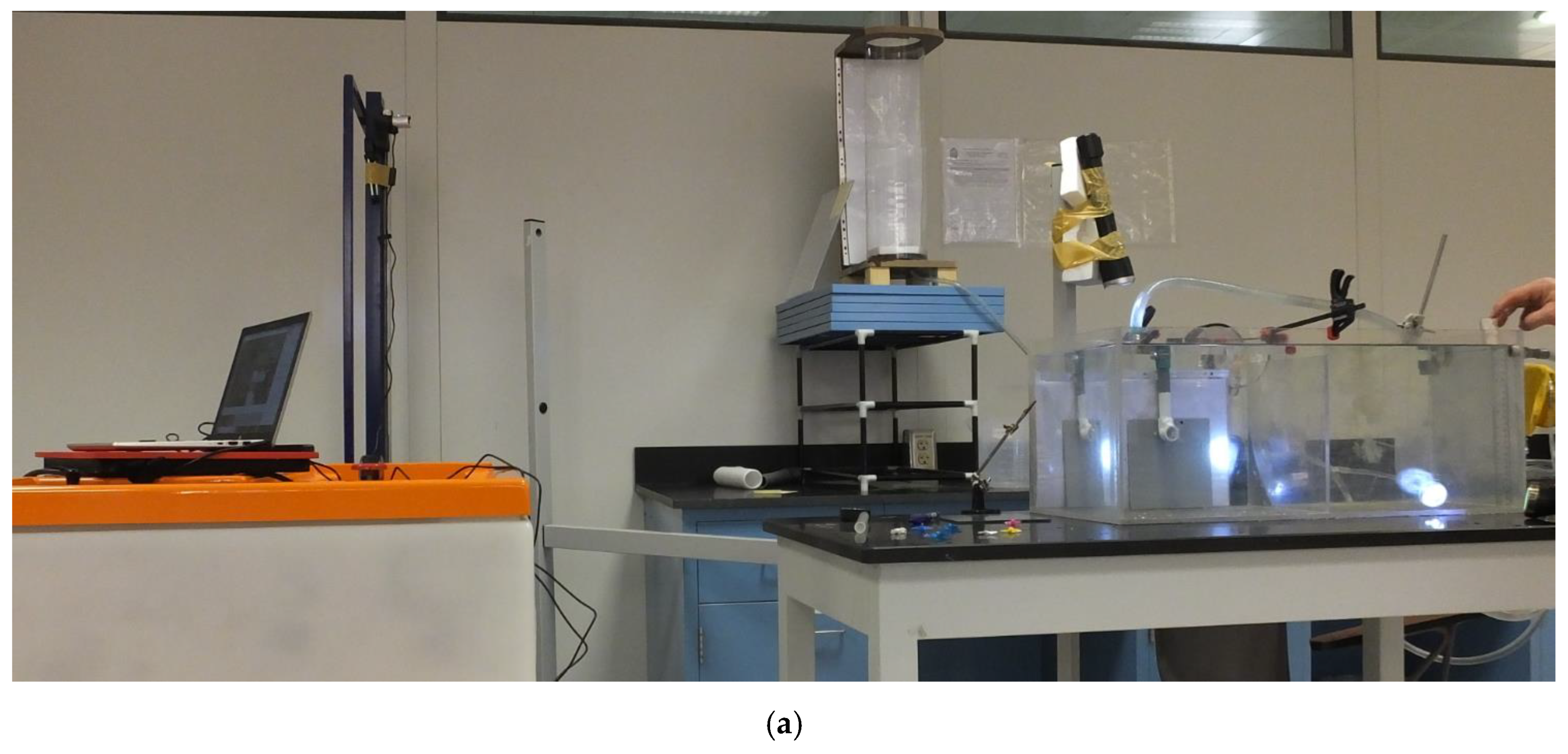
Figure 1 shows the experimental setup. The system consists of a vertical cylindrical feeding tank (tank 1) made of plexiglass. The tank height is 68 cm, and the tank diameter is 14 cm. The tank’s base is elevated about 30 cm above the water surface in the constant head mixing tank (tank 2). Tank 2 is a prismatic plexiglass tank with horizontal dimensions of 69 cm × 30.5 cm, and its height is 28 cm. The tank consists of two compartments of similar size, and they are separated by a side internal plexiglass baffle that works as a side weir of a crest height that equals 24.2 cm. The effluent water of tank 1 is transmitted to the left compartment of tank 2 via a PVC transparent pipe that ends by an 18 mm diameter pipe outlet. The pipe outlet is submerged under the constant head water surface in tank 2. Water moves from the first compartment to the second compartment via the internal side weir. The second compartment is provided by a circular outlet discharge pipe to drain the excess water to keep the water elevation in the left tank compartment constant.
2.2. List of Experimental Runs
Eight experiments were conducted to study the effect of adding a passive rotor (to the pipe outlet of a tank-gravity pipe system) on the system’s hydraulic performance. Table 1 shows the characteristics of those runs.
The main variables considered for experimental investigation include the rotor size, number of blades, and the symmetry of the blade. It should be noted that the blades are considered symmetric if the angles between any two successive blades are the same and constant. Based on this definition, the rotor used in run 4 is asymmetric, and except for run 4, all the other runs were provided with rotors with equally angled blades (i.e., symmetric rotors).
2.3. Cameras and Apparatus
2.3.1. Digital Cameras
Two digital cameras were used for data acquisition. The first camera is a bridge-type Fuji Finepix digital camera used to capture the temporal variation of the rotor’s angular speed. The second camera is a Microsoft LifeCam Studio webcam used to capture the water level’s temporal variation in tank 1. The main characteristics of both cameras are given in Table 2 [15,16].
2.3.2. High Flux Spotlight
It is well known that shooting at a high frame rate requires more intense lighting. For instance, shooting at 1000 fps involves light 5.25 times more than shooting at a standard frame rate (25 fps). Therefore, video recording at relatively high-speed rates (240 to 480 fps) requires additional light (compared to the typical shooting at 25–30 fps) to avoid black scenes. Thus, two torches of DC concentrated LED Flux light were used for camera 1. The inclination angles of the light beams were adjusted by trials to prevent or minimize undesirable shadows (Figure 1b).
2.4. Video Tracking Packages
Video analysis and tracking could be conducted manually or automatically. The manual tracking of the object of interest could be achieved by using frame-by-frame video analysis software. The automatic tracking could be carried out using the general image processing packages or toolboxes such as MATLAB/OCTAVE image processing toolbox/package. It can also be conducted directly using the video analysis packages that were specifically developed to track the motion of an object throughout a captured video and have the auto-tracking option. Examples of auto-tracking packages include Vernier, Tracker, Logger Pro, and many others [17,18].
Tracker is a freeware video analysis and modeling tool package developed in 2010 by Brown as an Open-Source Physics project (O.S.P.) [19]. In this study, Tracker software (version 5.1.5) was used for analyzing all video data by both cameras.
Auto tracking of an object or a feature in a recorded video clip can be conducted by Tracker. This involves creating a featured image called a “template image” for the selected moving feature of interest by the user, then the package starts searching each frame in the recorded video for the best match to that template image. To achieve this, two main numerical parameters need to be set. The first is the “match score” parameter, and the second is the “evolution rate percentage”. The default values for these parameters are 4 and 20%, respectively. The first parameter is necessary to identify the best match template image, whereas the second parameter is used to consider the possible temporal changes that might occur for the shape and colors of the template image. It should be mentioned that adapting higher values for the evolution rate may result in template “drift” over many frames. In this study, the default value for the match score was used for all runs, whereas a minimum value of 5% for the evolution rate was adopted for all the water level tracking runs to avoid the template image “drift” problem [20].
2.5. Measurement of Angular Speed
The angular speed of the rotating rotor is one of the parameters that need to be measured. Different approaches can be found in the literature to measure angular speed, including tachometers, stroboscopes, and, more recently, video analysis and tracking [17,18,21].
Measuring the angular speed using the video tracking method relies on a relatively high-speed frame capturing camera to track a relatively small marker on the revolving object. The merits of using the video analysis method are threefold. First, it is low cost as the measurement can be conducted by even a mobile camera equipped with slow-motion technology. Moreover, a number of point-and-shoot digital cameras or bridge cameras are currently available in the market at low cost (under USD 300), and they are capable of recording good-resolution images at fast frame rates. Second, the video analysis method is non-intrusive for the flow field, and it can be used to conduct measurements for submerged objects. Third, the video analysis technique gives the time-averaged angular speed values and the corresponding temporal perturbations/fluctuations around the time-averaged values. Elgamal et al. [18] presented a table that gives guidelines for selecting the required minimum frame per second (fps) rate for the relevant camera to attain a resolution capable of capturing the temporal variations of the angular speed rate.
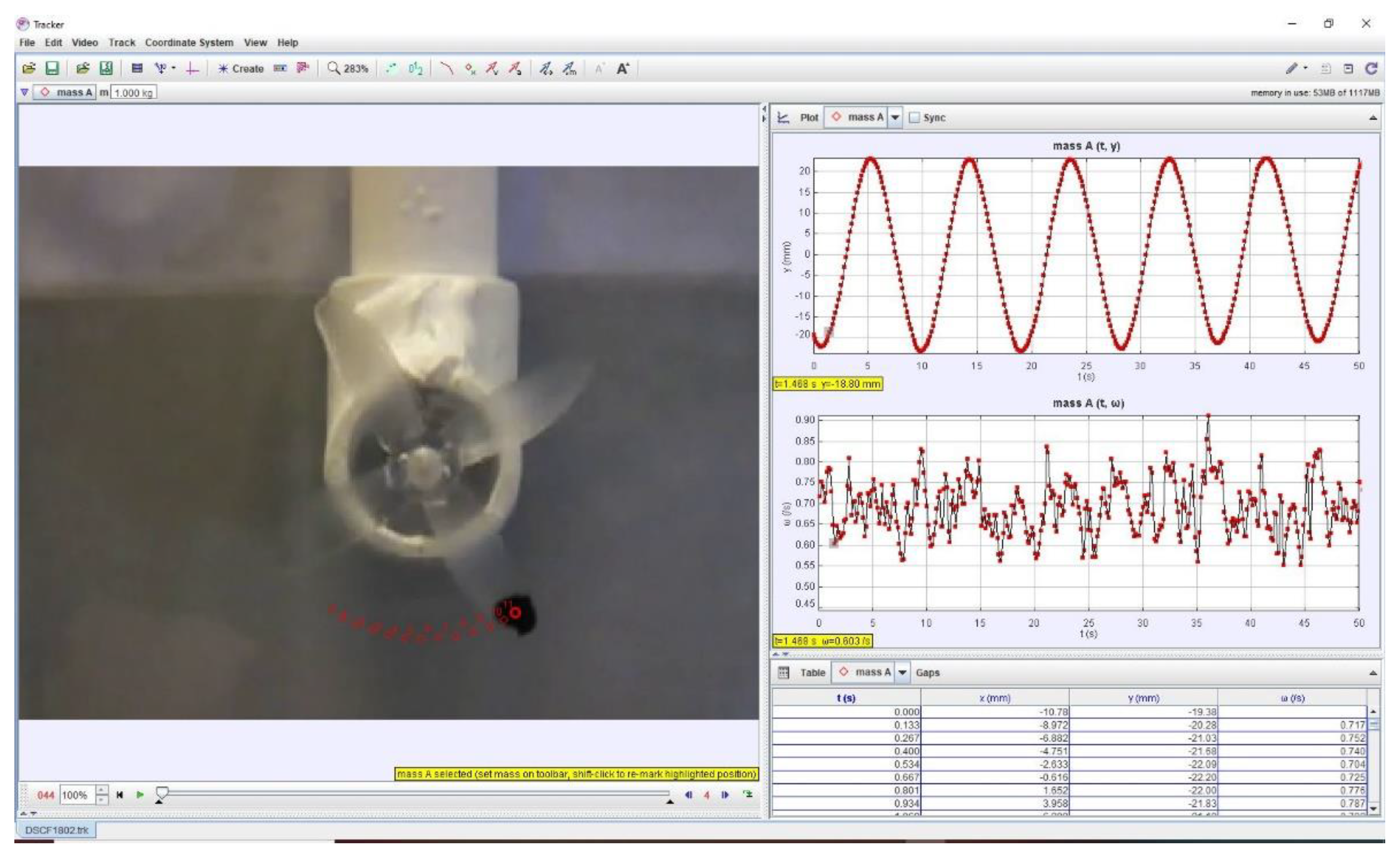
To measure the angular speed using the Tracker package, a circular dot marker of radius 2 mm is drawn on the tip of one of the rotor’s blades. The dot marker is auto-tracked via Tracker, and the temporal variation of the x and y coordinates of the marker is identified and plotted, as shown in Figure 2. The figure also shows the typical results of the auto-tracking procedure performed by Tracker. The dot marker coordinates were then internally used by Tracker to determine the instantaneous variations of the angular speed. The time-averaged values of the angular speed were calculated by applying the moving window average technique while considering an average time of one second.
2.6. Measurement of Water Level and Orifice Flow
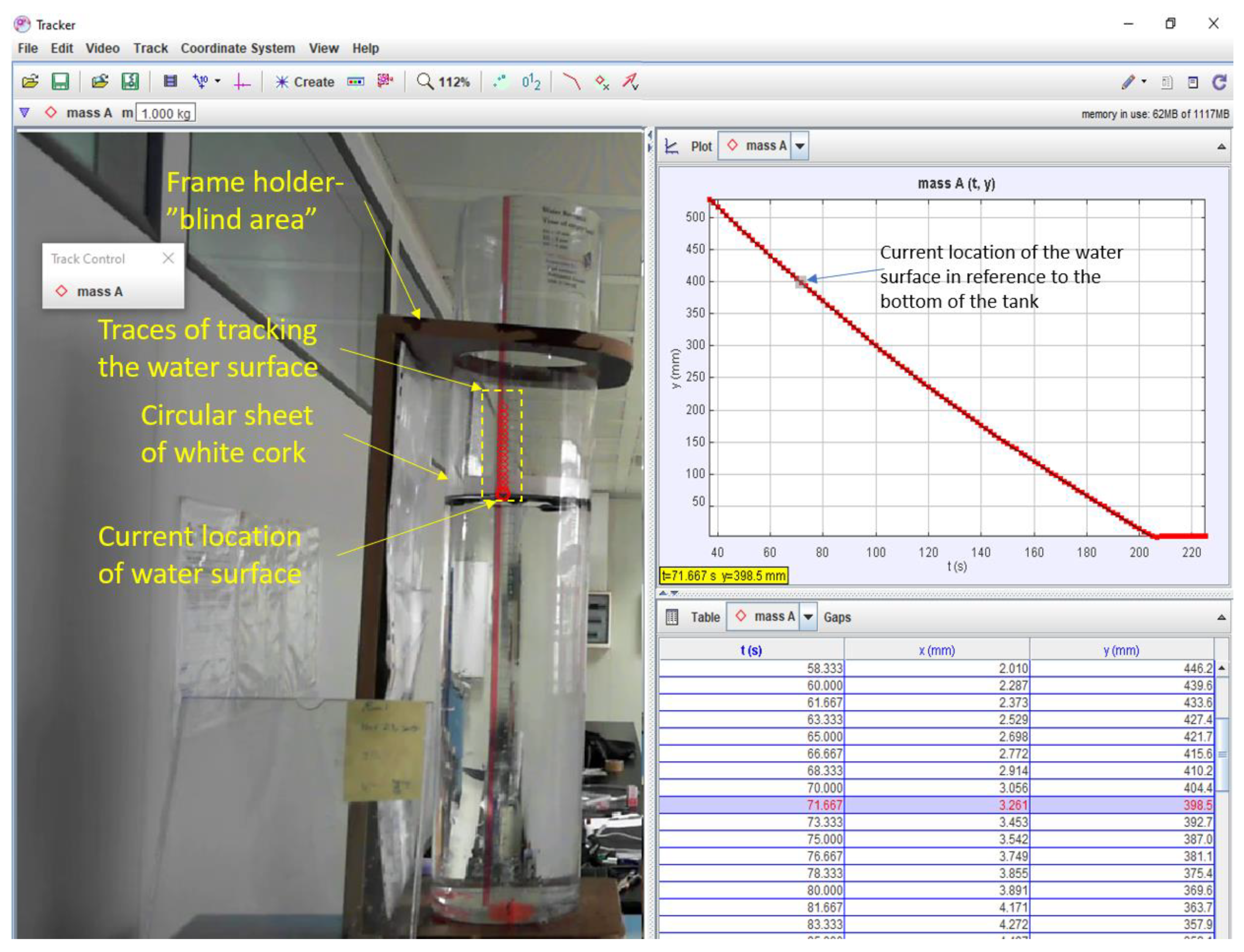
The water level in tank 1 was measured using the webcam camera (camera 2, refer to Figure 1b). The measurement is based on adding a light floating object (made of a white cork sheet) on the water surface and tracking the interface between the floating object and water surface using the Tracker package. To ease the tracking, the lower surface of the cork sheet was painted black. Tracker has two searching schemes to search for the best match for the template image. The first is the looking ahead method, and the second is searching only in the x-direction. Since the tank’s falling water level is along the vertical direction only, it was essential to constrain the tracking process along the vertical direction only. A simple trick to achieve this is to rotate the default x-axis in Tracker to point down the vertical direction.
The advantages of the measurement method mentioned above are twofold. First, it is inexpensive to do, as cheap devices like a webcam could be used. Second, the technique can capture high temporal variations in the water surface without any additional equipment.
Figure 3 shows a typical example of auto-tracking the water surface in the falling tank using Tracker. It should be noted that the horizontal holder of tank 1 formed a “camera blinded area”; therefore, tracking was switched off throughout that area, and after passing it, the auto-tracking is switched on again.
The exit water flow can be indirectly measured by the volume-time approach, where the instantaneous flow rate can be calculated by dividing the reduction in the stored water volume in tank 1 by the elapsed time of water surface decline.
2.7. Main Assumptions
We consider the following principal assumptions:
- -
- Tap fresh water was used in all experimental runs. The effect of using a brine or hot water will be discussed in a follow-up paper;
- -
- The rotor center is set to be concentric with the center of the pipe outlet for all studied cases;
- -
- The downstream distance from the pipe outlet to the rotor (Lr, refer to Figure 1c) was found to be a crucial parameter that significantly affected the system behavior; however, the effect of this parameter is not investigated in the current work, and all runs were conducted with an equal distance gap (Lr/do = 0.75 ± 0.05);
- -
- -
- The time gap between the start of the water level decline (in tank 1) and the onset of the rotor’s rotation is negligible. Therefore, both videos captured by cameras 1 and 2 were manually synchronized;
- -
- Water is incompressible, and the transient flow variations within the PVC pipe will be ignored since the pipe length is short and its diameter is small. Moreover, all experiments were conducted after removing all trapped air in the system;
- -
- The water temperature is 24 degrees Celsius, the water density = 0.9973 gm/cm2, and kinematic viscosity n = 0.00914 cm2/s.
2.8. Work Flow
The workflow for all experimental runs includes the following steps:
- -
- turn on both cameras 1 and 2;
- -
- open valves 1 and 2 and fill tank 1 using the submersible pump;
- -
- slightly open valve 3 to remove all trapped air in the system then close it again;
- -
- adjust the settings of cameras 1 and 2 (refer to Section 3.5), then start video recording;
- -
- completely and rapidly open valve 3 until the complete drainage of tank 1;
- -
- turn off both cameras after the end of the experiment;
- -
- convert the recorded files into lower-resolution mp4 files to avoid crashing the Tracker package. The required conversion was done by the Shotcut video editing package [22]. Attention should be given to deactivate the parallel processing option in the Shotcut package during conversion to avoid having choppy videos in the playback;
- -
- time-track the water surface in tank 1 (by Tracker) using recorded video by camera 2;
- -
- time-track the rotor’s angular speed (by Tracker) using recorded video by camera 1;
- -
- plot temporal variations of tank 1 water depth and angular speed of the rotor, then carry out post-processing analysis.
3. Numerical Analysis
The temporal variations of the tank’s exit flow and rotor’s angular speed are highly dependent on the declining trend of the tank water depth. Therefore, it is crucial to get a formula that describes the water decline trend. The reasons to use the numerical approach are twofold. First, no analytical solution is found for the water decline trend due to the non-linearity of the pipeline’s friction term in the tank-pipe outlet system. Second, it is difficult and impractical to use the experimental approach because of the large number of variables that need to be examined. Accordingly, the numerical approach will be applied to numerically seek a closed-form equation that describes the declining trend of the tank water depth.
First, the governing equations of the numerical approach are introduced, then calibration for the experimental setup based on data measurements of run 1 is conducted to compare measurements with the calculations and to get the pipe roughness value that gives the best match. Next, a large number of numerical runs will be conducted to examine the sensitivity of the declining trend. This sensitivity analysis aims to identify the dominating variables and dimensionless pi-terms that highly affect the declining trend of the normalized tank water depth. This finding will directly help obtain a closed form for the declining trend of the tank water depth in a tank-pipe outlet system.
3.1. Emptying Time for a Tank-Orifice System
Estimating the time required to drain a tank is one of the old problems generally handled in elementary fluid mechanics courses [23]. The problem is simply solved for the tank-orifice system, but it is, on the other hand, pretty implicit, non-linear, and with no compact analytical solution for the tank-pipe-outlet system.
If the tank ends by an orifice and the tank cross-section is constant, then the problem becomes straightforward, and the analytical solution of the time of emptying the tank could be easily obtained by integrating the incremental time required to discharge an incremental volume of water within the tank. In this regard, Euler or Bernoulli equation is used for the integration step, and the emptying time is obtained as shown in Equation (1) [23].
where:
- Teo is the time of emptying a tank-orifice system;
- A is the cross-section area of the tank (tank 1 while replacing the pipe outlet by an orifice outlet);
- Cdo is the orifice coefficient of discharge;
- Ho is the maximum water depth in the tank (tank 1);
- g is the acceleration of gravity;
- ao is the orifice flow area (for the tank-orifice system) or the pipe outlet area for the tank-pipe-outlet system).
3.2. Governing Equations for a Tank-Pipe-Outlet System
In a tank-pipe-outlet system, it will be challenging to get an analytical solution for emptying the tank partly because of the non-linearity of the friction term related to the pipeline element. To overcome this challenge, the numerical analysis will be applied using the governing equations given below.
For the no passive rotor case, the outlet flow, Q, can be derived from the energy equation to give Equation (2):
where:
Cd is the “lump sum” discharge coefficient, and it is given by Equation (3):
where:
- λ is the local-losses-to-friction-losses ratio;
- L is the pipe length from tank 1 to the pipe outlet;
- d is the pipe diameter;
- do is the diameter of the pipe outlet (L);
- dr is the diameter of the rotor (L);
- a is the pipeline flow area (a = );
- A is the cross-section area of tank 1 (A = );
- D is the diameter of the cross-section of the tank;
f is the friction coefficient, which can be obtained from White’s and Brook equation or explicitly from the Swamee and Jain formula, Equation (4):
where:
- ks is the pipe roughness height;
- Re is the Reynolds number (Re = Qd/aν);
- ν is the kinematic viscosity of water.
3.3. Calculation of Exit Flow from the Pipe Outlet
From mass conservation and since only water exits from tank 1 during the experiment, the water level in the tank can be used to get the exit flow by using the ordinary differential Equation (5):
where t is the elapsed time variable since the start of tank drainage.
The set of Equations (2)–(5) can be used to determine the emptying time of a tank, the temporal variations of the water depth in the tank, and the exit discharge from the pipe outlet over time. The equations are algebraic-ordinary differential implicit-nonlinear equations and can be solved using a simple finite difference Euler time-discretization scheme.
3.4. Calibration of the Tank-Pipe-Outlet System (No Rotor Case)
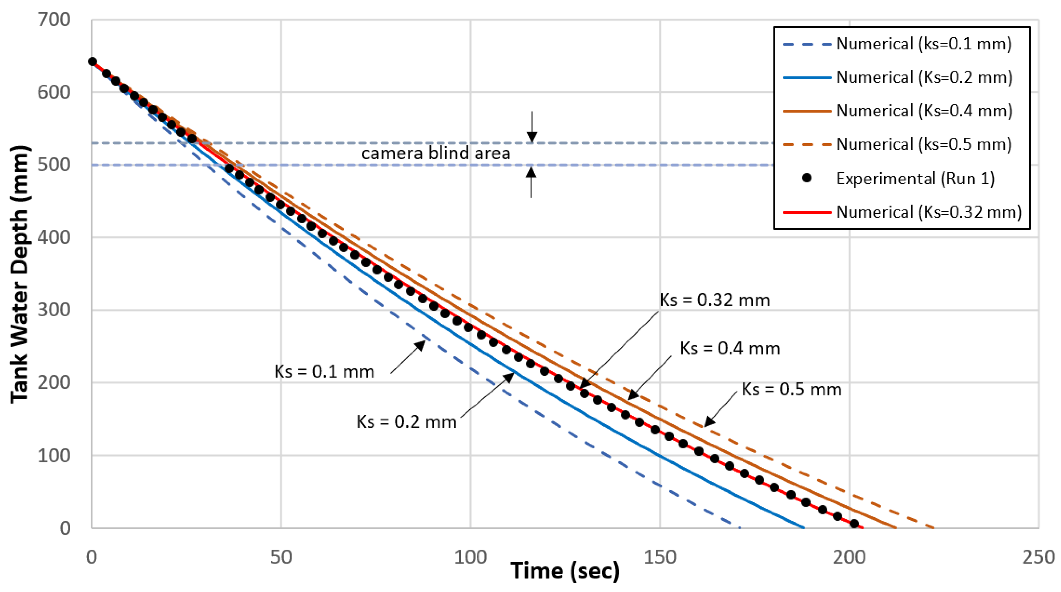
Before proceeding further in the numerical analysis, it is essential to identify the actual roughness of the pipeline element. The Tracker package was used to perform water depth measurements according to the methodology presented in Section 2.6. Figure 4 shows the temporal variation of the water depth in tank 1 for the no rotor case (run 1). A numerical calculation was conducted to solve Equations (2)–(5) using finite-difference with a time increment (∆t) of 0.1 s. The ratio of the local losses to the friction losses (λ) is set to be equal to 0.1, and the automatic iterative option was enabled (setting the maximum number of iterations to be 10 iterations) to overcome the non-linearity/implicitness that resulted from the dependence of the friction coefficient on the flow. Figure 4 also shows the calculated decline in the water depth for the different pipe roughness values tried, from 0.1 mm to 0.5 mm. A pipe roughness of 0.32 mm gives the best match with the measurements. The calculation revealed that the time it takes to empty the tank initially filled at a water depth Ho = 642 mm is about 203 s.
Figure 4.
System calibration (run 1 with no rotor).

The good match between measurements and calculations (shown in Figure 4) reveals that the set of equations (Equations (2)–(5)) accurately describes the declining trend of the water depth in tank 1.
3.5. Sensitivity Analysis for Parameters Affecting the Falling Trend of the Water Depth
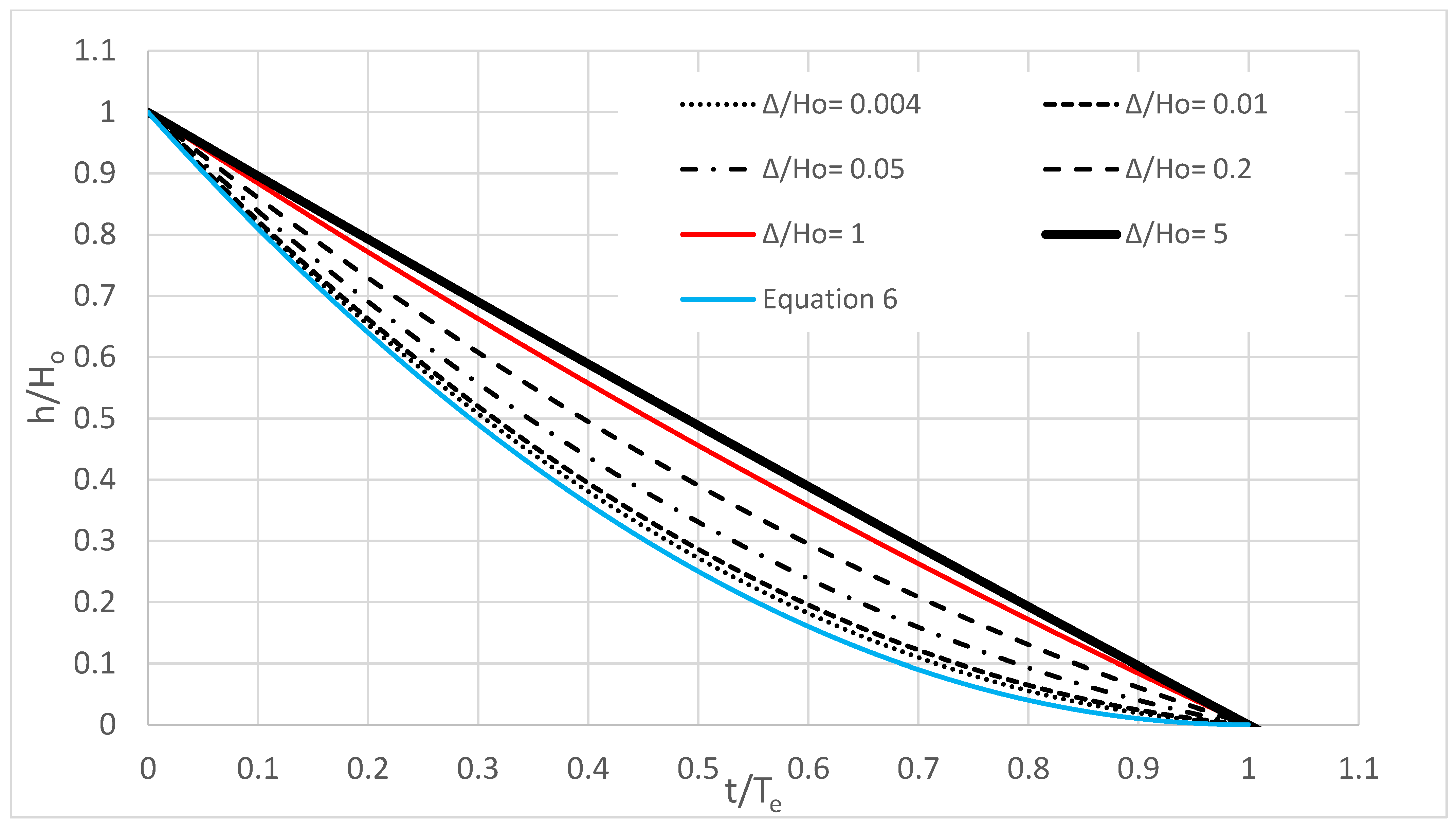
Identifying the falling trend of the water depth in a tank is also vital for tank water level control operations. It is vital to obtain a universal relation (if any) that describes the declining trend of the normalized water depth in the tank for different hydraulic parameters. In 2003, Libii derived the falling trend of water draining slowly from a large tank with an orifice outlet. He was able to get an analytical solution for the water falling trend after neglecting the acceleration of the water-free surface compared to the acceleration of gravity. The obtained falling trend is given by Equation (6) [24].
It will be challenging to get an analytical solution for the falling water trend in a tank-pipe-outlet system due to the non-linearity of the friction term related to the pipeline element. To overcome this challenge, the numerical analysis could be used. To achieve this, 157 numerical runs were conducted using the numerical approach described in Section 3.2. The sensitivities of the hydraulic parameters Ho, ∆, D, L, d, and ks were examined using the range of variance shown in Table 3.
The sensitivity analysis results have revealed that the water decline trend is affected by two dimensionless pi-terms. These pi-terms are ∆/Ho and Ld/D2. The first pi-term strongly affects the water decline trend (refer to Figure 5) while the second pi-term has a marginal effect.
Figure 5 shows the decline trends of the dimensionless water depth in a tank-pipe-outlet system for different ∆/Ho values. Figure 5 also compares the decline trends for the tank-pipeline-outlet system (derived numerically) and the corresponding trend for the tank-orifice system (derived analytically by Libii, Equation (6)). It is clear that as ∆/Ho gets smaller, the decay trends line gets closer to the trend line given by Equation (6). Interestingly, in the case of smaller values of ∆/Ho (refer for instance to the curve for the case of ∆/Ho ≥ 0.004), it is possible to drain the water of the last 27% of the tank volume in 50% of Te. On the contrary, for higher values of ∆/Ho (for instance, ∆/Ho ≥ 5), it is possible to drain the last 50% of the tank volume in 50% of the complete Te. The finding, as mentioned above, could be explained as follows: for a given Ho value, increasing ∆/Ho implies increasing the pressure head on the pipe outlet, resulting in faster drainage for the remaining water volume in the tank.
Figure 5 also shows that for ∆/Ho < 5, the declining trend is parabolic. On the other hand, for ∆/Ho > 5, the declining trend can be reasonably described as a linear relation. Based on that discussion, a normalized universal decline trend for the water depth in a tank-pipe-outlet system can be given by:
where:
- Te: is the time required for fully emptying the tank-pipe-outlet system with no rotor;
- Ter is the time it takes to empty a tank-pipe-outlet system with a passive rotor;
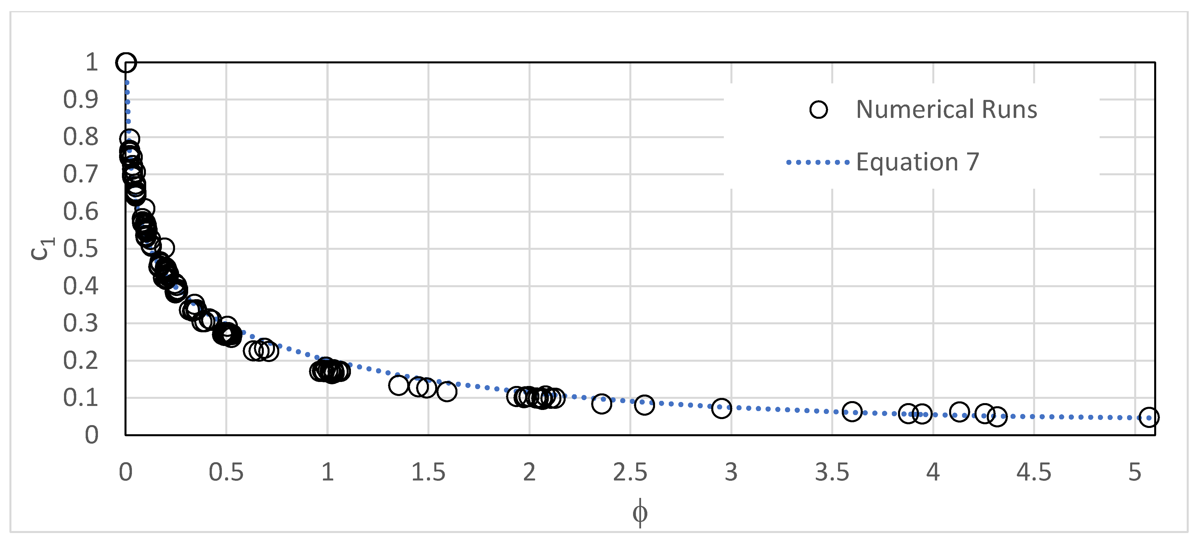
- c1 is a coefficient that depends on a function and can be determined using Equation (8) or (9);
- c2 and c3 are constants given by Equation (10).
For
where is a dimensionless parameter that combines the two dominating pi-terms identified from the sensitivity analysis; its relation is given by Equation (11).
Figure 6 shows the best match of Equation (7) with all the numerical runs conducted for the 0.0 ≤ ∆/Ho ≤ 5.1 range.
It should be mentioned that Equations (7)–(11) comprise a set of equations that can be used to get a universal closed-form relation for the falling trend of the dimensionless water depth.
4. Results and Analysis
This section presents the results of the experimental and numerical runs. Discussion of the findings is presented in Section 5.
4.1. Temporal Variation of Tank Water Depth (with Rotor Cases)
Figure 7 presents the tank water depth measurements using different passive rotors downstream of the pipe outlet as per Table 2. Figure 7b provides a “zoom in” shot for the lower parts of the given curves in Figure 7a. Based on Figure 7, and by comparing all the curves with the reference “no-rotor curve” (i.e., run 1), it is clear that adding a passive rotor downstream of the pipe outlet generally helped in decreasing the tank emptying times (Te), except for run 4 with asymmetric blades. The noted decrease in the emptying time could be justified by forming a low-pressure zone at the pipe outlet due to the mutual water-rotor interactions. The local pressure drop will be referred to hereafter as the induced local pressure drop (∆p) at the location of the pipe outlet. The induced local pressure drop increases the exit flow, thereby decreasing the emptying time. Further discussion about the local induced drop in the pressure will be given later on.
Figure 8 presents the decline trends for the normalized tank water depth over all the conducted runs (run 1 to run 8). The x-axis presents the elapsed time since the commencement of drainage normalized by the total time of emptying (Ter). Figure 8 indicates that adding the passive rotor does not apparently change the temporal decline trend of the tank water depth. This implies that Equation (7) could also be applied for the outlets with passive rotors.
4.2. Outlet Flow and Induced Pressure
4.2.1. Temporal Variation of Tank Outlet Flow (with Rotor Cases)
The outlet water flow could be determined from the tank water depth measurements using Equation (5). It is important to note that using Equation (5) implicitly means neglecting all the transient/storage effects in the pipe that connects the tank and the pipe outlet. This assumption seems reasonable in the case of short pipe lengths and small pipe diameters. By substituting Equation (6) in (5) and differentiating with time, one can obtain the following normalized linear equation, Equation (12), that describes the temporal variation of the exit flow from the pipe outlet:
where ADR is the time-averaged drainage rate (in mL/s), and it is calculated using Equation (13).
where ADRo is the reference value of ADR, which presents the average drainage rate of a tank connected to a pipe with no passive rotor (similar to run 1). Te and Ter are the times of emptying tanks for without and with a rotor, respectively.
4.2.2. Effect of a Passive Rotor on Tank Average Drainage Rate
To study the effect of adding a passive rotor to a pipe outlet, a new dimensionless number called the Normalized difference in Average Drainage Rate (NADR) has been introduced as:
As is clear from Equation (14), the NADR is a dimensionless number that gives the expected change in the average drainage rate due to using a passive rotor. If NADR is positive, then the actual ADR is greater than the reference value (no rotor case, ADRo), and vice versa is also correct.
By substituting Equation (13) in Equation (14), the time of emptying ratio (Ter/Te) could be obtained as:
Based on Equation (14), it is possible to rewrite Equation (12) as:
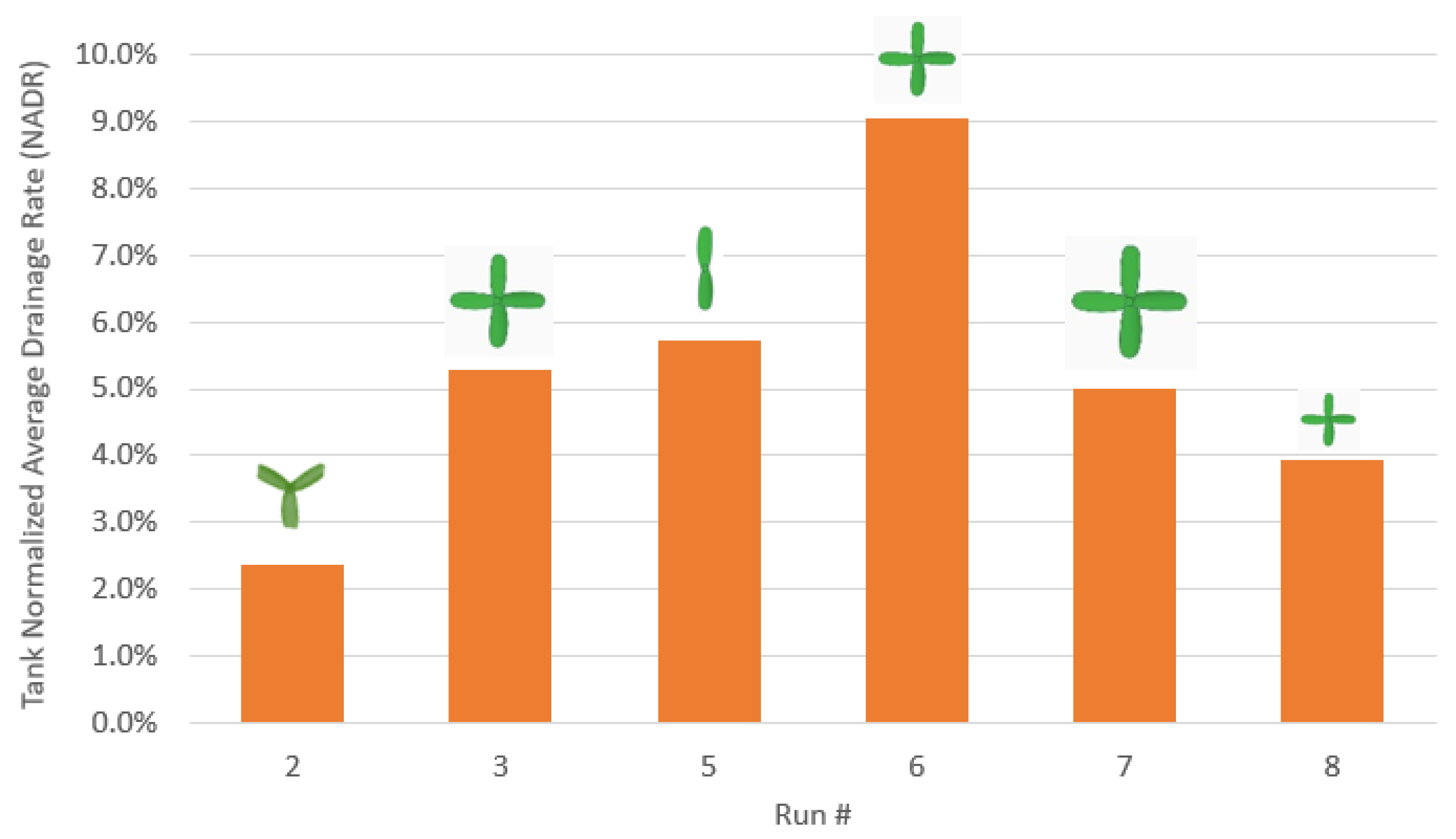
Figure 9 presents how NADR varies for all the runs, including tanks supplied with passive rotors of symmetric blades.
It is important to note that adding passive rotors with symmetric blades causes the average drainage rate to increase by up to 9.0%, as shown in Figure 9.
4.2.3. Induced Drop in Pressure at Pipe Outlet
Introducing a passive rotor downstream of a pipe outlet will convert the problem from a conventional pipe outlet to an unconventional outlet with a water–structure interaction behavior. As a result of this mutual interaction, a zone of reduced pressure extended from the pipe outlet to the rotor is expected to form. More details about that will be presented in the discussion.
Accordingly, Equation (2) could be revised to include the pressure loss as:
Q = Cd.a√(2g(h + ∆ + |∆p/γ|))
By substituting Equation (16) into Equation (17), an analytical formula that gives the induced pressure drop could be obtained, as given in Equation (18):
The analytical formula for the induced pressure drop needs to be verified experimentally and numerically. An initial CFD study carried out by the authors has confirmed the induced pressure drop due to the revolving action of the rotor. However, discrepancies between Equation (18) and the CFD result are noticed. More research effort is required to evaluate the accuracy of Equation (18).
4.3. Effect of Rotor Size and Symmetricity
4.3.1. Rotor Size
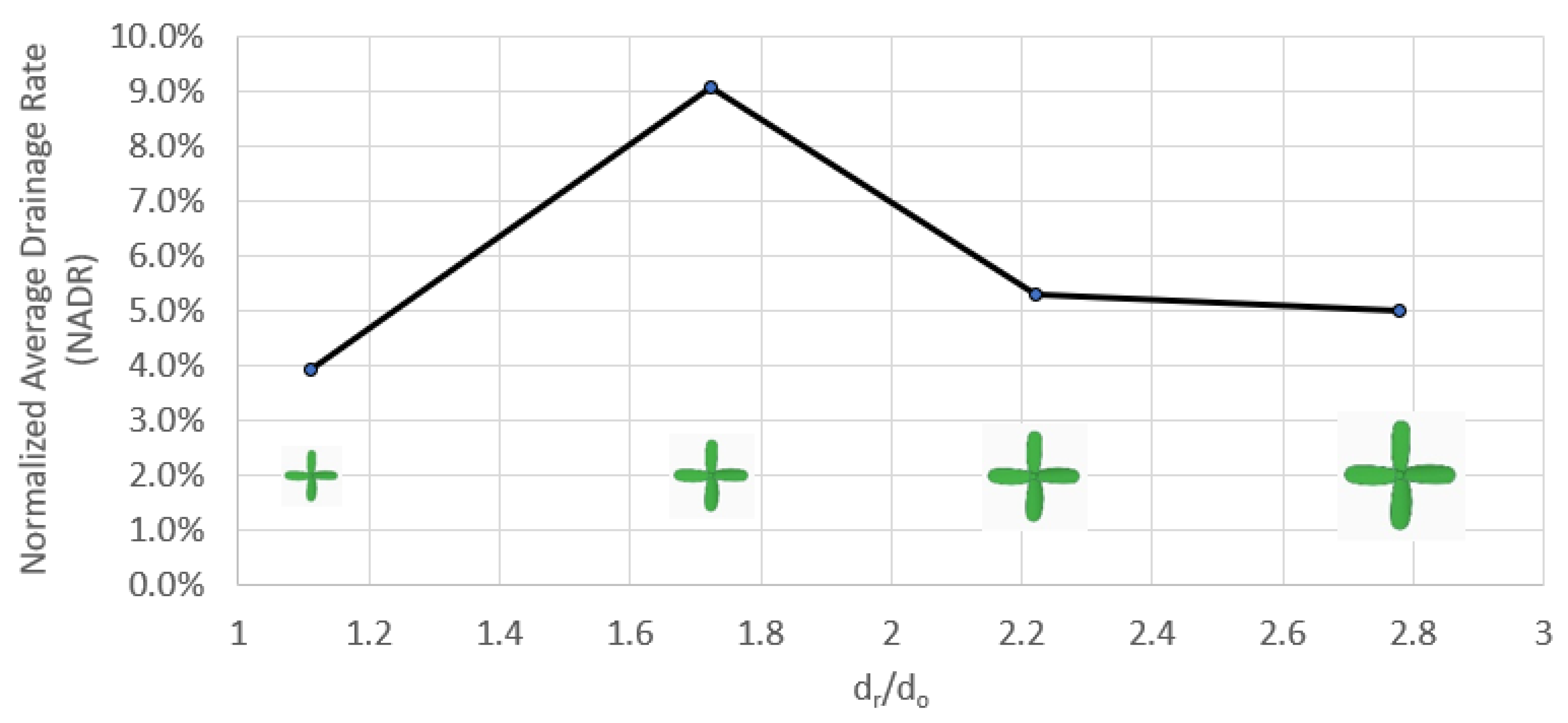
To study the effect of the rotor size on enhancing the ADR, four-blade rotors with different blade sizes were used. Figure 10 shows the effect of using different blade sizes on enhancing the ADR for the 4-blades rotors only. The x-axis represents the rotor size (dr) normalized by the pipe outlet’s diameter (do). It is crucial to mention that the maximum enhancement in ADR occurs when the rotor’s size is 1.73 times the pipe outlet’s size.
4.3.2. Rotor Symmetricity
It is of interest to investigate the impact of a broken rotor blade (for any reason) on the drainage rate. To examine this situation, run 4 is added to the experiments list (refer to Table 2). In run 4, a three-blade passive rotor was used with unequal angles between blades (asymmetric setting of blades). Due to the asymmetric blade rotor, significant perturbation in the passive rotor rotation took place. To ensure accurate results, run 4 was repeated several times to check repeatability and identify its performance range. Figure 11 presents the effect of rotor asymmetry on the NADR for the cases where rotor size equals dr/do = 1.73. The water depth measurements in all runs were also repeated to examine repeatability, and the shown error bars give the corresponding range of variance. Analysis of the water level measurements for run 4 demonstrated that NADR values range from 1.45% to −1.37%. This means that switching from the symmetric four blades to the asymmetric three-blade rotor significantly reduces NADR. If another blade is broken (in a way that the rotor became symmetric with two blades, i.e., run 5), the system perturbation will be reduced, causing NADR to increase again.
4.4. Temporal Variation of Angular Speed
Figure 12 shows a typical example of the temporal variation of the ensemble average of the angular speed (ω) of the rotor for the base run (run 6). The temporal variations present three distinct stages. The first is the acceleration stage (from A to B), where the angular speed of the rotor accelerates from stillness to its maximum speed, reached at point B (ωmax = 340 rpm). During this stage, the rotor is accelerating, although the pipe flow is decelerating. The second stage is the first rotor decelerating phase (from B to C), where the rotor starts to linearly and gradually decelerate with time. At point C, the tank is completely drained, and the transmission pipe starts to rapidly drain until it reaches point D. The rapid deceleration of the angular speed can be explained by the significant difference between the tank cross-section area (A) and the pipe cross-section area (a).
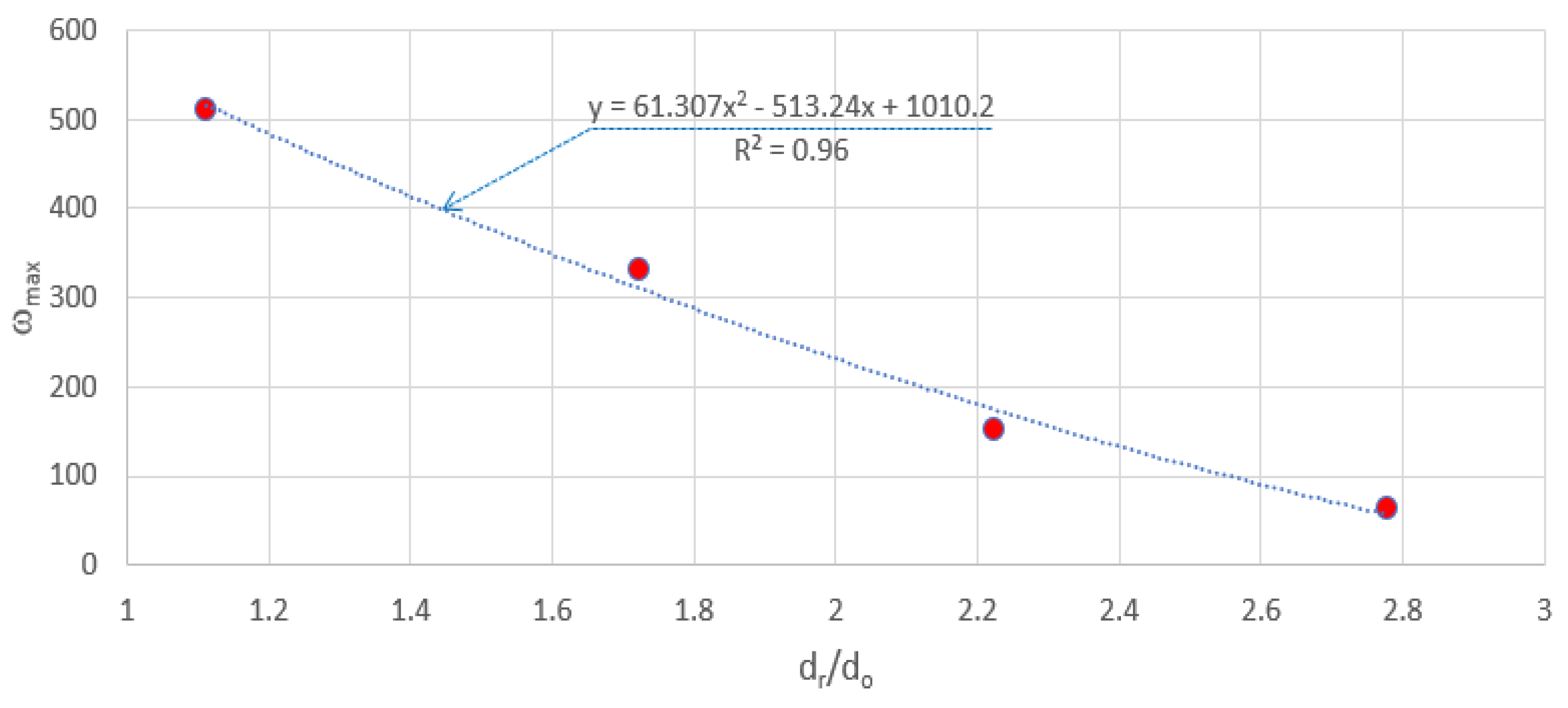
Figure 13 presents the temporal variations of the normalized rotor’s angular speed (ω/ωmax) for the 4-blade rotors. It is noted that within the gradual deceleration stage, ω/ωmax generally decreases linearly from unity to about 0.4. The maximum angular speed is found to inversely decrease with the rotor’s size ratio (dr/do), as shown in Figure 14.
It is interesting to compare the tip rotor speed (Vr = ω.dr/2) with the outlet water velocity (Vo = 4Q/πdo2). In this regard, the tip rotor speed ratio (α) is defined as:
Figure 15 presents the temporal variations of α for different rotor sizes. For instance, the figure shows that the tip rotor speed is almost twice as fast as the outlet water velocity for the case of dr/do ≈ 1. It is interesting to note that the temporal variations of α are not significant or nearly constant within the decelerating stage (B to C).
The maximum and time-averaged values of α can be obtained from the trends given in Figure 16. It is worth mentioning that the time-averaged tip rotor’s speed ratio for the rotor size that produces the maximum NADR is about 1.65.
5. Discussion
This paper proposes the use of a passive rotor at the pipe outlet to enhance the system performance of a tank-pipe-outlet system. Following an experimental approach, the paper presented an integrated system of measurement comprising two digital cameras and a video analysis and tracking tool (Figure 1b). The system is inexpensive, simple, and allows non-intrusive measurement for the temporal variations of the water depth in the tank, the exit flow, and the passive rotor’s speed. The proposed system of measurement is expected to be a useful tool for studying more sophisticated transient applications.
The study shows that, in tank-pipe-outlet systems, the normalized falling trend of the water depth is parabolic with time. The numerical runs have shown that the coefficient (c1) of the second-order term of the falling trend is strongly dependent on the ratio ∆/Ho (refer to Figure 5); however, it is marginally dependent on the pi-term Ld/D2 (refer to Figure 6). For a given initial water depth in the tank (Ho), as ∆ increases, the pressure on the pipe outlet increases, causing the exit velocity to rise and tank drainage to become higher. Therefore, the falling trend becomes less parabolic and more linear as the ratio (∆/Ho) increases (Figure 5).
One of the interesting findings of the conducted experiments is that adding a rotor to the pipe outlet does not change the falling trend of the tank water depth (Figure 8); however, it results in a shorter time of emptying and a higher drainage rate. The reduction of the time of emptying could be explained as follows: when a passive rotor is added at the pipe outlet, it starts rotating due to the energy transfer and momentum exchange from the exit water flow. Rotation of the rotor has the following effects on the outlet system:
- First, the rotor will partly act as a liquid displacement unit that is continuously displacing/washing away the water from the front of the pipe outlet, and this will help in reducing the effect of outlet-submergence on the drained flow, and consequently, it will result in increasing the exit flow;
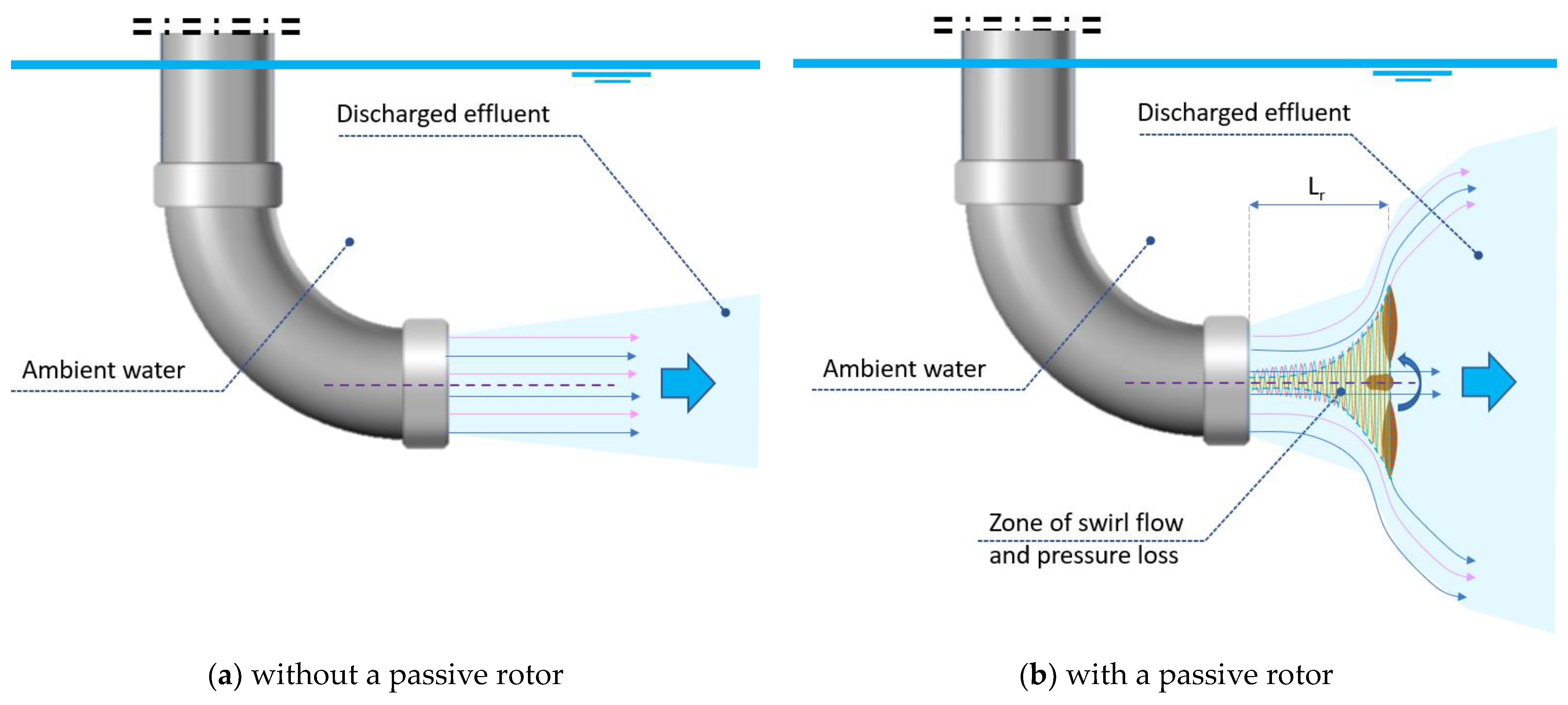
- Second, because of the small distance between the pipe outlet and the rotor blades (Lr/do = 0.75), a swirl flow is established dominated by the action of the revolving rotor. The swirl flow helps in forming a zone of low pressure that extends from the tips of the rotor to the pipe outlet (Figure 17b). The reduction of the pressure at the pipe outlet is responsible for increasing the exit flow and the water tank average drainage rate (ADR). Figure 17a,b illustrate the schematic presentations of the expected flow fields for the “without” and “with rotor” cases, respectively.
In order to easily quantify the passive rotor effect on the tank-pipe-outlet system, the normalized averaged drainage rate (NADR) is introduced. Having this single number in hand, a designer can obtain valuable information about the system performance following these steps:
- (1)
- (Select the size of the rotor. A designer could use the optimal size of the 4-blade rotor (dr = 1.73 do) to maximize the drainage rate, or any other relevant rotor size;
- (2)
- (3)
- Determine the emptying time ratio (Ter/Te) based on Equation (15);
- (4)
- Solve Equations (2)–(5) numerically to calculate the tank time of emptying (Te) assuming that the outlet has no passive rotor;
- (5)
- Calculate Ter, using Te and the emptying time ratio (Ter/Te) from step (3);
- (6)
- Use Equations (7) and (16) to calculate the temporal variations of the water depth and exit flow, respectively;
- (7)
- Based on the rotor size, use Figure 16 to determine the time-averaged tip-to-rotor-speed ratio; thus, the temporal variation of the angular speed can be also identified using Equations (16) and (19).
6. Conclusions
In this study, the hydraulic effect of introducing a passive rotor to a tank-pipe-outlet system was investigated experimentally to assess its effect on the tank drainage rate and the hydraulic performance of the outlet. A number of rotors with different sizes and a number of blades were used. The temporal variations of the tank water depth and the rotor’s angular speed were recorded using two digital cameras to enable relatively high-speed imaging. Video analysis and image processing were performed using the Tracker package to determine the temporal variations of the tank water depth and the corresponding rotor’s angular speed.
The research findings have generally shown that:
- Adding a symmetric passive rotor (with equally spaced angles between blades) helped increase the average water drainage rate (ADR) in the tank by up to 9.0% (compared to the no passive rotor case). The measured increase in the ADR is explained by the generation of a low-pressure zone at the pipe outlet due to the swirl flow induced by the water–rotor mutual interactions.
- The optimum size for a 4-blade symmetric rotor that produces the highest increase in ADR is when the rotor diameter is 1.73 times the pipe outlet’s diameter (i.e., dr/do = 1.73).
- Using asymmetric rotors (i.e., 3-blades with unequal angles) could adversely impact the ADR due to the significant perturbation produced by the rotor asymmetricity.
- A closed-form formula for the decline trend of the dimensionless water depth in a tank-pipe-outlet system was obtained based on a semi-experimental and numerical approach.
- Tracking the angular speed of the passive rotor has revealed that the rotor’s angular speed increases as the rotor size decreases.
- When a tank-pipe-outlet system starts to drain, the rotor’s angular speed rapidly increases from stall before reaching a maximum value; then, the rotor’s angular speed decreases noticeably as water depth declines to complete tank drainage.
- The tip rotor speed (Vr) could be faster than the exit water velocity from the pipe outlet. For a four-blade rotor with dimensions of dr/do = 1.73, it is found that the tip rotor speed exceeds the exit water velocity by 65% (i.e., α = 1.65).
- The temporal variation of the tip rotor’s speed ratio is insignificant during the water depth falling, and it can be assumed constant. This finding can be used to get a direct relation between the exit discharge and the rotor’s angular speed.
7. Challenges, Limitations, and Outlook
Using the passive rotor might be challenging in some situations. One of these situations is the case where the disposed water contains a high load of sediment. The high sediment load might affect the rotor’s angular speed and thus the performance of the whole system at large. More research efforts should be dedicated to addressing this effect.
Besides the challenges, there are several limitations in the current study. For instance, the current experiments disregarded the thermal and density difference effects of the disposed water on the passive rotor. This point should be addressed in future work. Another limitation is related to using an elbow (in the experimental setup) close to the outlet (as seen in Figure 1b). This might have a strong influence on the performance of the rotor. Therefore, it is generally recommended to avoid using any fittings close to the rotor, to ensure uniformity in the flow field. This practice is expected to enhance the rotor’s mixing performance.
The water–rotor mutual interaction was narrowly investigated in the current work. The presented analytical formula for the induced pressure drop (Equation (17)) must be verified experimentally and numerically. The distance between the rotor and the outlet (Lr) seems to significantly affect the system performance. However, this effect needs to be identified to come up with the optimum Lr value that results in the system’s best performance.
Despite the challenges and limitations discussed above, the findings of the study in hand are crucial, and they are viewed as prerequisites for future investigations devoted to examining the mixing behavior of a passive rotor added to an outlet that discharges thermal or brine pollutants.
Author Contributions
Conceptualization, M.E. and K.K.; methodology, M.E., M.F. and K.K.; software, M.E. and M.F.; validation, M.E. and M.F.; formal analysis, M.E. and M.F.; investigation, M.E. and K.K.; resources, K.K.; data curation, K.K.; writing—original draft preparation, M.E.; writing—review and editing, M.E., M.F. and K.K.; visualization, M.E. and K.K.; supervision, M.F.; project administration, M.F.; funding acquisition, M.F. All authors have read and agreed to the published version of the manuscript.
Funding
This research was supported by the Deanship of Scientific Research, Imam Mohammad Ibn Saud Islamic University, Saudi Arabia, Grant No. 20-13-14-003.
Institutional Review Board Statement
Not applicable.
Informed Consent Statement
Not applicable.
Data Availability Statement
Data are available on request from the authors.
Acknowledgments
This research was supported by the Deanship of Scientific Research, Imam Mohammad Ibn Saud Islamic University, Saudi Arabia, Grant No. 20-13-14-003. The authors would like to thank the Deanship of Scientific Research, Imam Mohammad Ibn Saud Islamic University, Saudi Arabia, for supporting and fund this research.
Conflicts of Interest
The authors declare no conflict of interest.
Abbreviations
| A | the cross-section area of tank 1, refer to Figure 1b (L2) |
| ADR | average drainage rate in case of using a passive rotor at the pipe outlet (L3/T) |
| ADRo | average drainage rate in case of having no passive rotor at the pipe outlet (L3/T) |
| a | the pipe cross-section, flow, area (L2) |
| ao | the orifice flow area (for the tank-orifice system) or the pipe outlet area for the tank-pipe-outlet system) (L2) |
| CFD | computational fluid dynamics |
| Cd | the discharge coefficient for the tank-pipe-outlet system [1] |
| Cdo | the orifice discharge coefficient for the tank-orifice system [1] |
| D | diameter of the water falling tank (tank 1) (L) |
| d | pipe diameter from the tank to the pipe outlet (L) |
| do | diameter of the pipe outlet (L) |
| dr | diameter of the rotor (L) |
| DC | direct current |
| f | the friction coefficient which can be obtained from Swamee and Jain formula [1] |
| g | the acceleration of gravity (L/T2) |
| h | the instantaneous water depth in tank 1 at time t (measured from the tank bottom) (L) |
| Ho | maximum water depth in the tank or the tank height (L) |
| L | the pipe length from tank 1 to the pipe outlet (L) |
| LED | light-emitting diode |
| Lr | distance from the pipe outlet to the rotor centroid (L) |
| NADR | normalized average drainage rate [1] |
| O.S.P. | open-source physics project |
| Q | instantaneous exit flow from the pipe outlet (L3/T) |
| Re | Reynolds number [1] |
| t | the elapsed time since the start of drainage (T) |
| Te | time of emptying a tank-pipe-outlet system with pipe outlet having no rotor (T) |
| Ter | time of emptying a tank-pipe-outlet system with pipe outlet having a passive rotor (T) |
| Teo | time of emptying a tank-orifice system with no rotor (T) |
| Vr | tip rotor speed (L/T) |
| Vo | outlet (exit) velocity of water flow (L/T) |
| α | the tip rotor’s speed ratio [1] |
| ∆ | the vertical distance between the water level in the constant head tank (tank 2) and the base of tank 1 (L) |
| λ | the ratio of the local losses to the friction losses [1] |
| ν | kinematic viscosity of water (L2/T) |
| ω | the time-averaged angular speed of a passive rotor (1/T) |
| ωmax | the maximum time-averaged angular speed of a passive rotor (1/T) |
References
- Water Outlet and Drain in Aquaculture Engineering. Available online: https://www.brainkart.com/article/Water-outlet-or-drain---Aquaculture-Engineering_15094/ (accessed on 5 May 2021).
- Roberts, P.J.W.; Salas, H.J.; Reiff, F.M.; Libhaber, M.; Labbe, A.; Thomson, J.C. Marine Wastewater Outfalls and Treatment Systems; IWA Publishing: London, UK, 2010; p. 9. ISBN 9781780401669. [Google Scholar] [CrossRef]
- Law, A.W.K.; Tang, C. Industrial water treatment and industrial marine outfalls: Achieving the right balance. Front. Chem. Sci. Eng. 2016, 10, 472–479. [Google Scholar] [CrossRef]
- Yan, X.; Mohammadian, A. Numerical modeling of multiple inclined dense jets discharged from moderately spaced ports. Water 2019, 11, 2077. [Google Scholar] [CrossRef] [Green Version]
- Adams, E.E.; Trowbridge, J.H. Near Field Performance of Staged Diffusers in Shallow Water; MIT Energy Laboratory: Cambridge, MA, USA, 1979. [Google Scholar]
- Mohammadian, A.; Kheirkhah Gildeh, H.; Nistor, I. CFD modeling of effluent discharges: A review of past numerical studies. Water 2020, 12, 856. [Google Scholar] [CrossRef] [Green Version]
- Tian, X.; Roberts, P.J.; Daviero, G.J. Marine wastewater discharges from multiport diffusers. I: Unstratified stationary water. J. Hydraul. Eng. 2004, 130, 1137–1146. [Google Scholar] [CrossRef]
- Tian, X.; Roberts, P.J.; Daviero, G.J. Marine wastewater discharges from multiport diffusers. II: Unstratified flowing water. J. Hydraul. Eng. 2004, 130, 1147–1155. [Google Scholar] [CrossRef]
- Abou-Elhaggag, M.E.; El-Gamal, M.H.; Farouk, M.I. Experimental and numerical investigation of desalination plant outfalls in limited disposal areas. J. Environ. Prot. 2011, 2, 828. [Google Scholar] [CrossRef] [Green Version]
- Inan, A. Modeling of Hydrodynamics and Dilution in Coastal Waters. Water 2019, 11, 83. [Google Scholar] [CrossRef] [Green Version]
- Yan, X.; Mohammadian, A.; Chen, X. Three-dimensional numerical simulations of buoyant jets discharged from a rosette-type multiport diffuser. J. Mar. Sci. Eng. 2019, 7, 409. [Google Scholar] [CrossRef] [Green Version]
- Samad, M.; El-Kheiashy, K. Effluent Mixing Modeling for Liquefied Natural Gas Outfalls in a Coastal Ecosystem. J. Mar. Sci. Eng. 2014, 2, 493–505. [Google Scholar] [CrossRef] [Green Version]
- Lyu, S.; Seo, I.W.; Do Kim, Y. Experimental investigation on behavior of multiple vertical buoyant jets discharged into a stagnant ambient. KSCE J. Civ. Eng. 2013, 17, 1820–1829. [Google Scholar] [CrossRef]
- Wang, H.J.; Davidson, M.J. Modeling merging jets in a coflowing environment. In Proceedings of the XXVIII IAHR Congress, Graz, Austria, 22–27 August 1999. [Google Scholar]
- Fuji FinePix HS50EXR Digital Camera, User Manual, BL01901-100. Available online: https://www.fujifilm.eu/fileadmin/product_migration/dc/downloads/HS50EXR_manuals_05.pdf (accessed on 12 April 2020).
- Microsoft LifeCam Studio WebCam, Data Sheet, Rev.1606A. 2016. Available online: https://download.microsoft.com/download/0/9/5/0952776D-7A26-40E1-80C4-76D73FC729DF/TDS_LifeCamStudio.pdf (accessed on 12 April 2020).
- Eadkhong, T.; Rajsadorn, R.; Jannual, P.; Danworaphong, S. Rotational dynamics with Tracker. Eur. J. Phys. 2012, 33, 615–622. Available online: http://iopscience.iop.org/article/10.1088/0143-0807/33/3/615/pdf (accessed on 17 May 2019). [CrossRef]
- Elgamal, M.; Abdel-Mageed, N.; Helmy, A.; Ghanem, A. Hydraulic performance of sluice gate with unloaded upstream rotor. Water SA 2017, 43, 563–572. [Google Scholar] [CrossRef] [Green Version]
- Brown, D. Tracker Introduction to Video Modeling (AAPT 2010). Portland, Oregon. 2010. Available online: http://www.compadre.org/Repository/document/ServeFile.cfm?ID=10188&DocID=1749 (accessed on 4 December 2019).
- Brown, D. Autotracker. 2010. Available online: https://physlets.org/tracker/help/autotracker.html (accessed on 21 December 2020).
- Robert, T. Video analysis—A multimedia tool for homework and class assignments. In Proceedings of the 12th International Conference on Multimedia in Physics Teaching and Learning, Wroclaw, Poland, 13–15 September 2007; Available online: http://www.mptl12.ifd.uni.wroc.pl/papers/63.pdf (accessed on 6 April 2020).
- Shotcut Getting Started Guides. Available online: https://shotcut.org/howtos/getting-started/ (accessed on 21 December 2020).
- Nakayama, Y. Introduction to Fluid Mechanics; Butterworth-Heinemann: Oxford, UK, 2018. [Google Scholar]
- Libii, J.N. Mechanics of the Slow Draining of a Large Tank under Gravity. Am. J. Phys. 2003, 71, 1204–1207. [Google Scholar] [CrossRef]
Figure 1.
Experimental setup: (a) snapshot of the experimental setup; (b) schematic of the experimental setup; (c) side view of a pipe outlet with a passive rotor; (d) front view of pipe outlet with a symmetric 4-blade rotor.
Figure 1.
Experimental setup: (a) snapshot of the experimental setup; (b) schematic of the experimental setup; (c) side view of a pipe outlet with a passive rotor; (d) front view of pipe outlet with a symmetric 4-blade rotor.

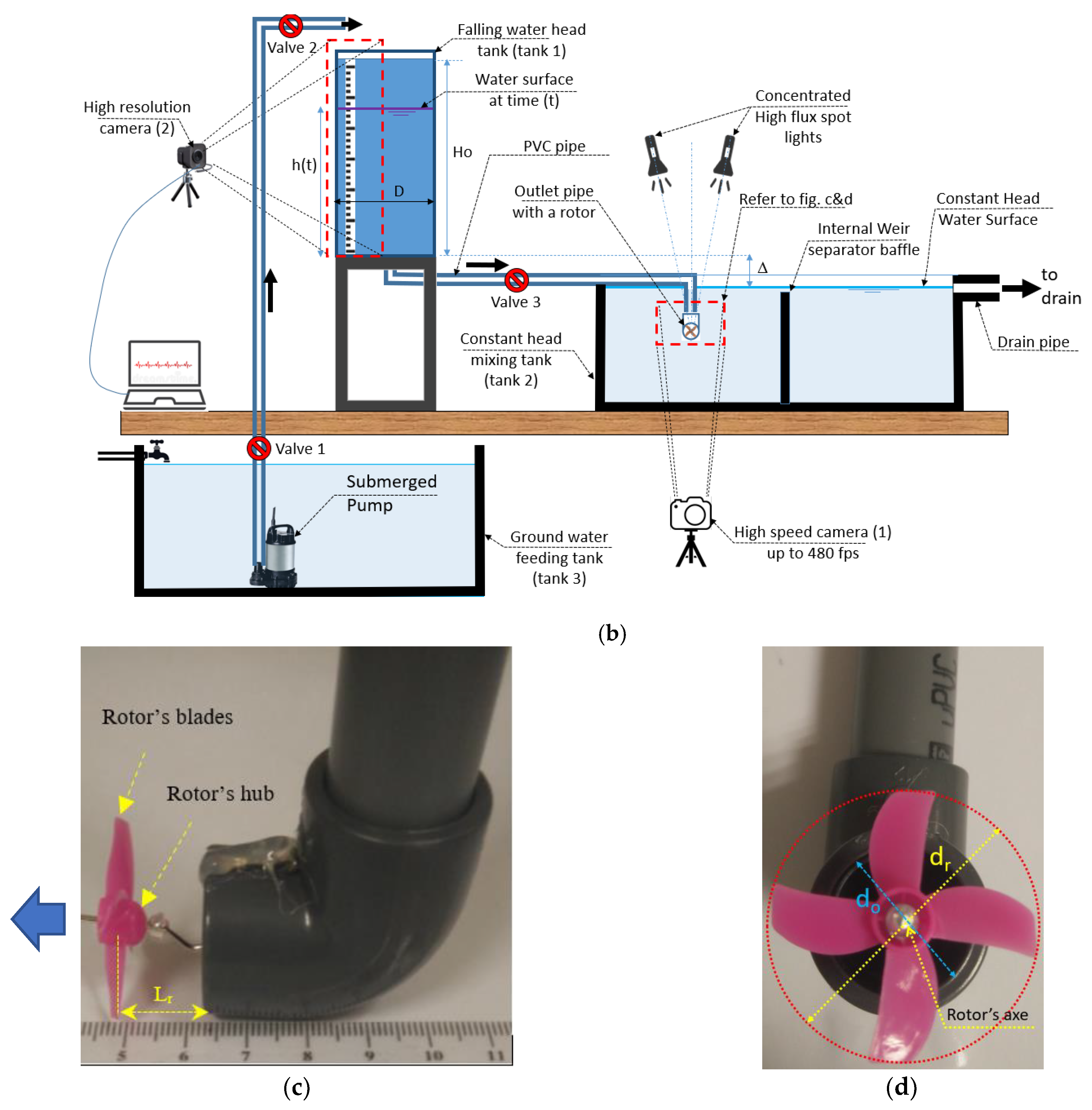
Figure 2.
Auto-tracking the dot circle marker via Tracker for the experimental runs.

Figure 3.
The process of auto-tracking the water surface in tank 1 via Tracker.

Figure 5.
Effect of ∆/Ho ratio on the decline trends for the tank water depth (tank-pipe-outlet system).
Figure 5.
Effect of ∆/Ho ratio on the decline trends for the tank water depth (tank-pipe-outlet system).

Figure 6.
Coefficient c1 as a function of ϕ (for ∆/Ho ≤ 5.1).

Figure 7.
Temporal variations of tank water depth using different passive rotors: (a) full data measurement range; (b) zoom in for the dashed window shown in panel a.
Figure 7.
Temporal variations of tank water depth using different passive rotors: (a) full data measurement range; (b) zoom in for the dashed window shown in panel a.
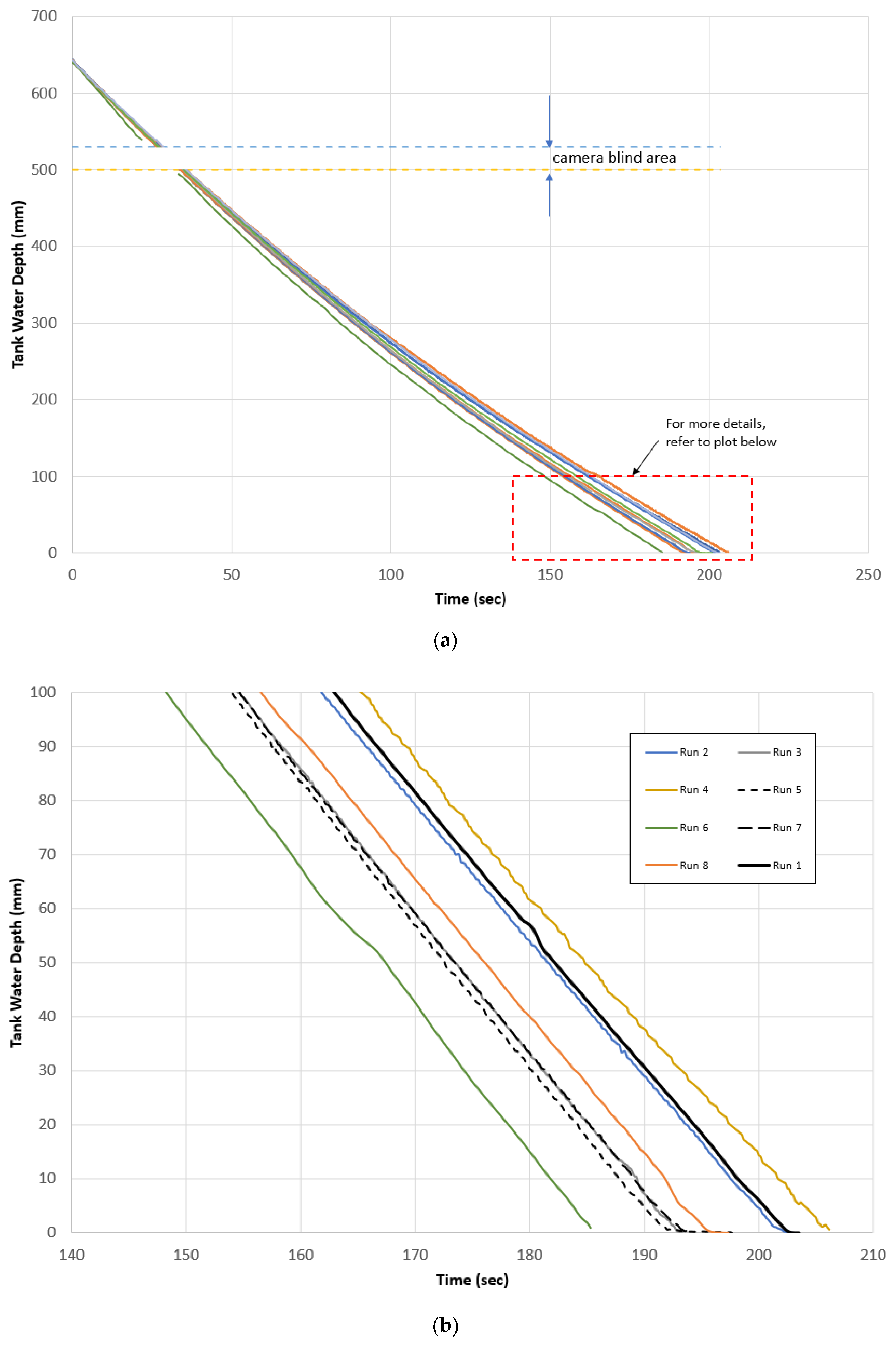
Figure 8.
The temporal decline trends for the normalized tank water depth with respect to time (with rotor).
Figure 8.
The temporal decline trends for the normalized tank water depth with respect to time (with rotor).
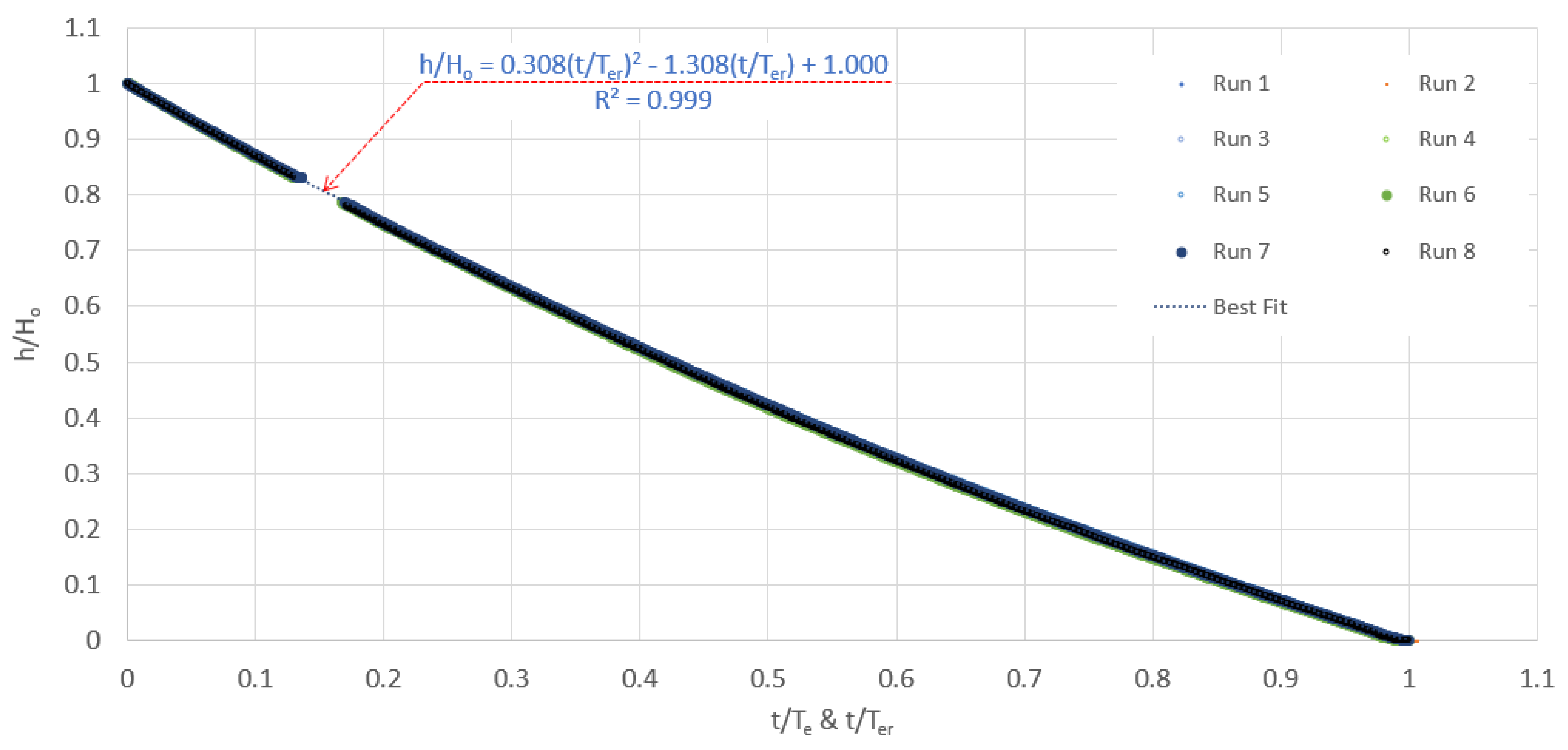
Figure 9.
Effect of using passive rotors with symmetric blades on average tank drainage rate.

Figure 10.
Effect of rotor size on the enhancement of tank drainage rate (4-blade rotors only).

Figure 11.
Effect of asymmetricity on the tank drainage rate (dr/do = 1.73).
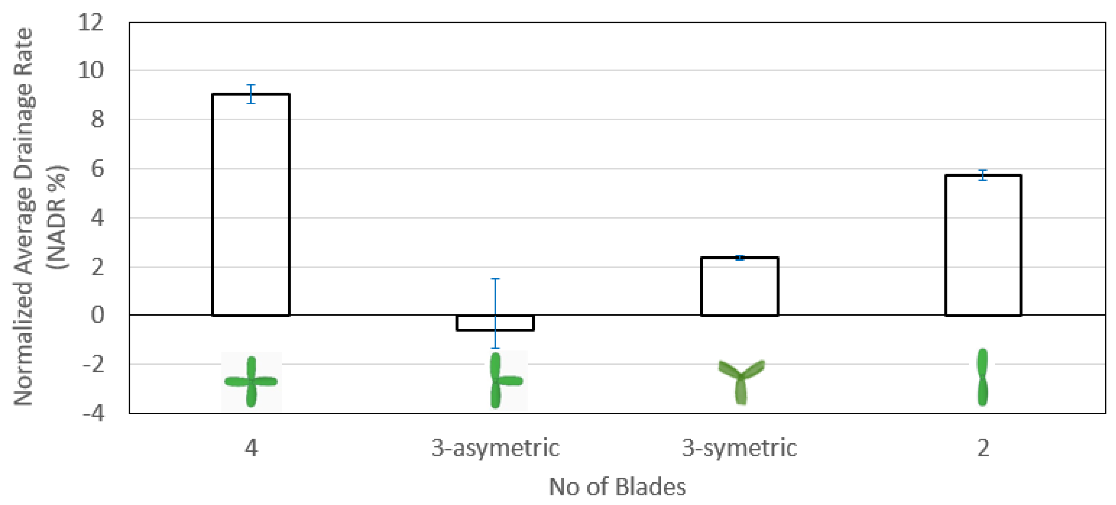
Figure 12.
Temporal variation of rotor’s angular speed (base run: run 6).
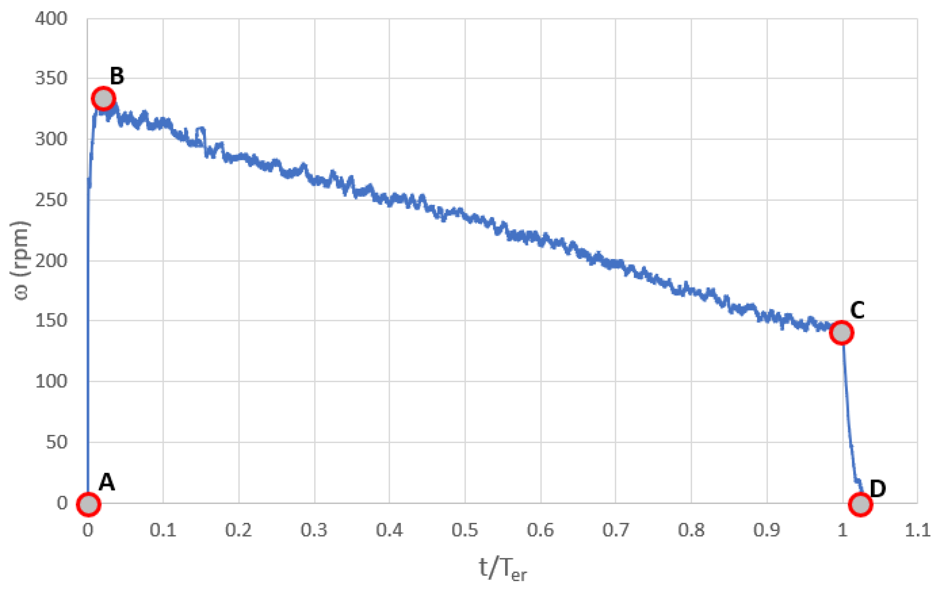
Figure 13.
Temporal variation of the normalized rotor’s angular speed (4-blade rotors).
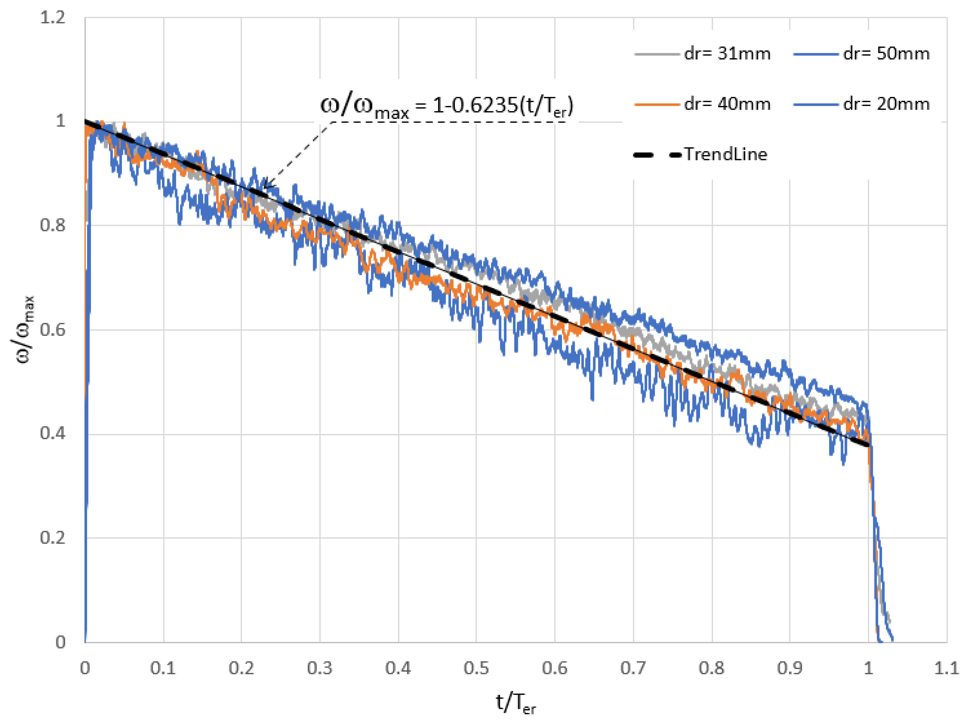
Figure 14.
Relation of the maximum rotor’s angular speed with the rotor’s size (4-blade rotors).

Figure 15.
Temporal variation of the tip rotor’s speed ratio (4-blade rotors).
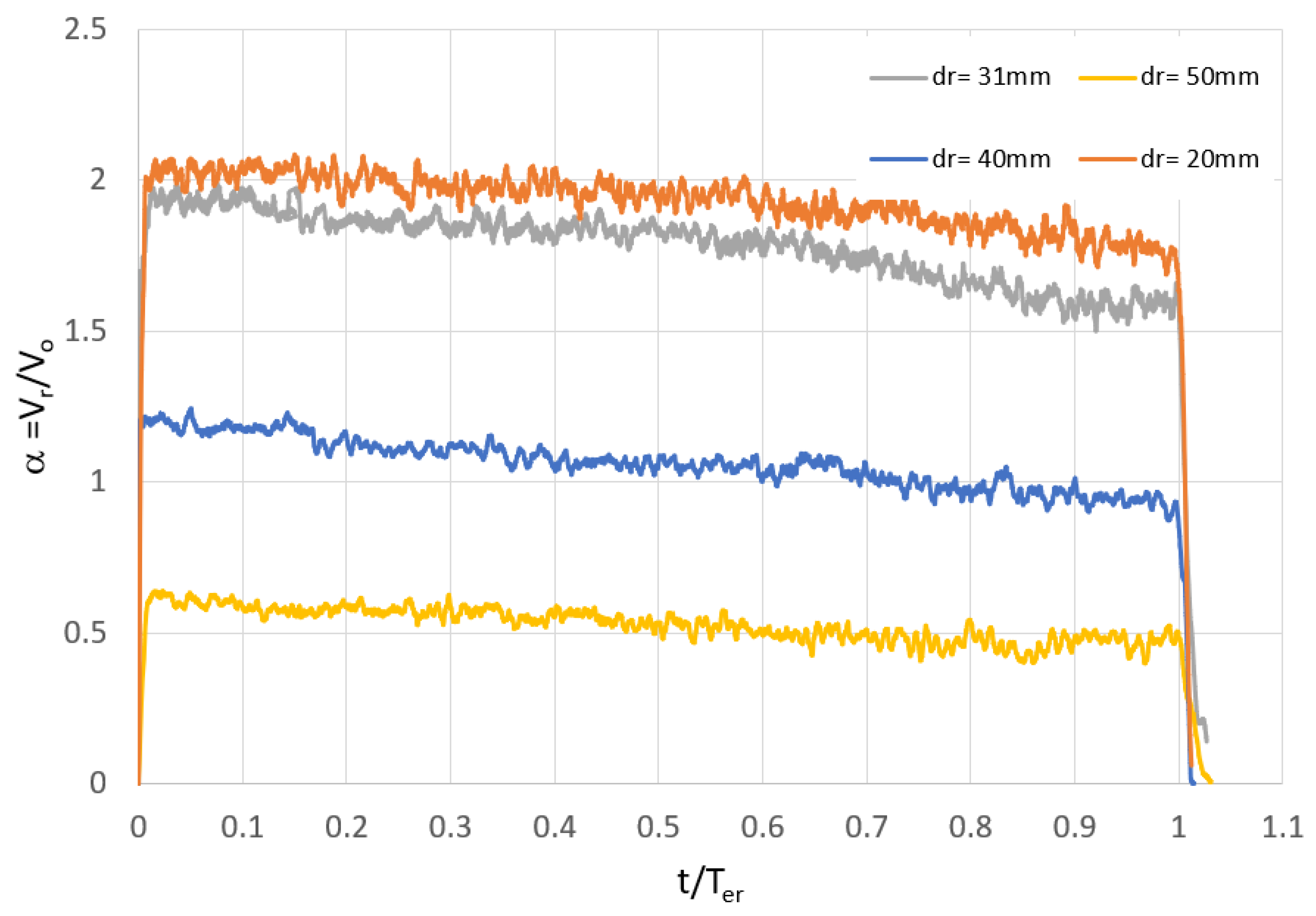
Figure 16.
Relations of the max/average tip rotor’s speed ratio with the rotor’s size (4-blade rotors).
Figure 16.
Relations of the max/average tip rotor’s speed ratio with the rotor’s size (4-blade rotors).
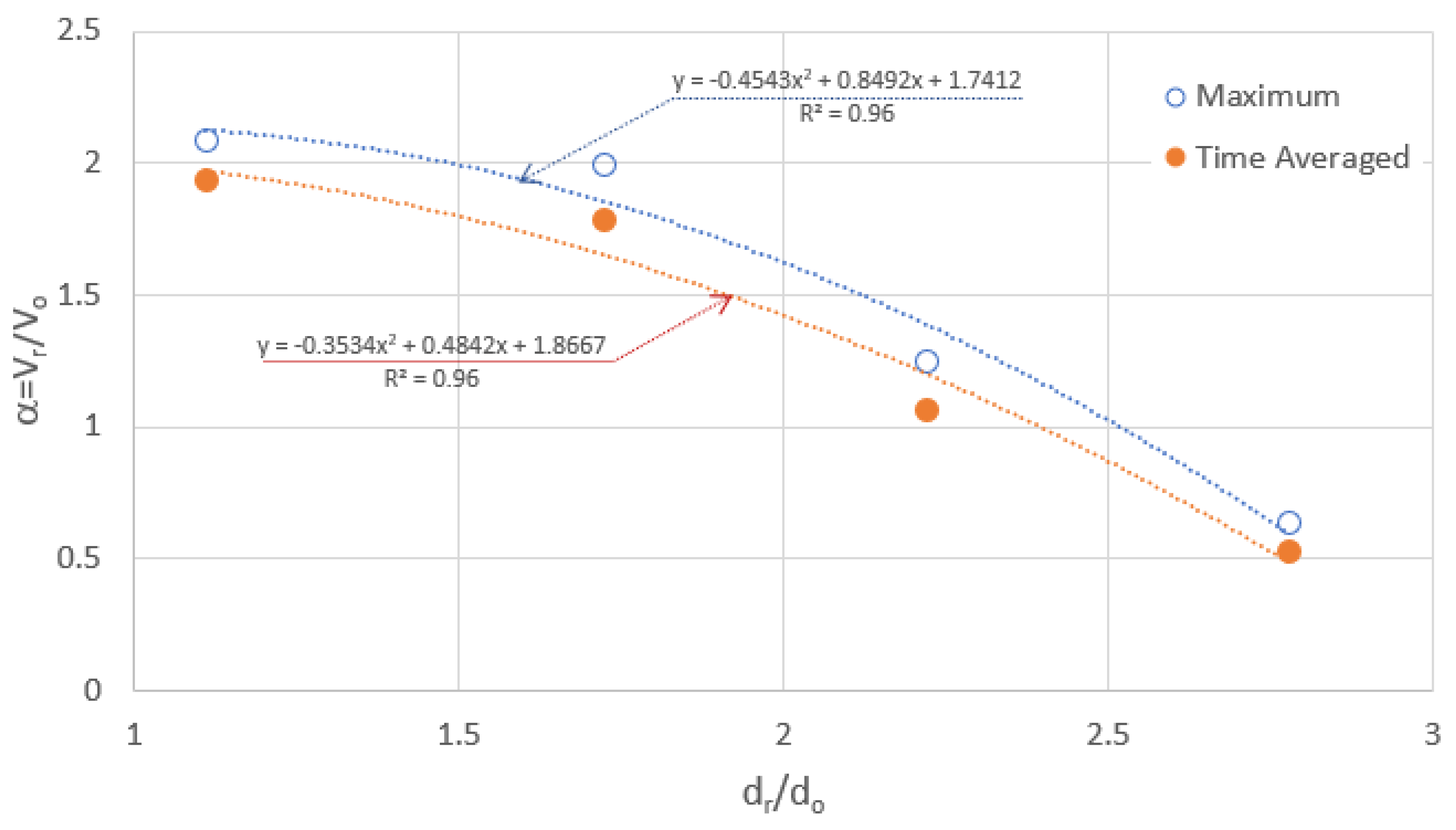
Figure 17.
Schematic presentation of the flow field downstream of a submerged pipe outlet.

Table 1.
Characteristics of the Conducted Experimental Runs.
| Run # | Run ID | Rotor Installed | Blades Symmetry | Blade Size (mm) | No of Blades | Rotor Shape | Comments | |||||||
|---|---|---|---|---|---|---|---|---|---|---|---|---|---|---|
| Yes | No | Yes | No | 20 | 31 | 40 | 50 | 2 | 3 | 4 | ||||
| 1 | FHB0D0SM | √ | NA | NA | Non | Reference Run | ||||||||
| 2 | FHB3D3SM | √ | √ | √ | √ |  | ||||||||
| 3 | FHB4D4SM | √ | √ | √ | √ |  | ||||||||
| 4 | FHB3D3SM | √ | √ | √ | √ |  | ||||||||
| 5 | FHB2D3SM | √ | √ | √ | √ |  | ||||||||
| 6 | FHB4D3SM | √ | √ | √ | √ |  | Base run | |||||||
| 7 | FHB4D5SM | √ | √ | √ | √ |  | ||||||||
| 8 | FHB4D2SM | √ | √ | √ | √ |  | ||||||||
Table 2.
Characteristics of Used Cameras.
| Item | Model | Type | Sensor | Max Resolution | Max Frame Rate | Measured Parameter | Accuracy |
|---|---|---|---|---|---|---|---|
| Camera 1 | FUJI-Finepix HS50EXR | Bridge | EXR CMOS-II | 16 Mega Pixel | 480 fps | angular speed | ±0.0042 s−1 |
| Camera 2 | Microsoft-LifeCam Studio | WebCam | CMOS | 5 Mega Pixel | 30 fps | water depth | ±0.11 mm |
Table 3.
Range of variability of examined hydraulic parameters.
| Variable | Ho (m) | D (m) | ∆ (m) | L (m) | d (mm) | Ks (mm) | |
|---|---|---|---|---|---|---|---|
| Range | Min | 0.5 | 0.14 | 0 | 4 | 10 | 0.1 |
| Max | 5 | 10 | 7 | 10,000 | 1000 | 1 | |
Publisher’s Note: MDPI stays neutral with regard to jurisdictional claims in published maps and institutional affiliations. |
© 2021 by the authors. Licensee MDPI, Basel, Switzerland. This article is an open access article distributed under the terms and conditions of the Creative Commons Attribution (CC BY) license (https://creativecommons.org/licenses/by/4.0/).
Share and Cite
MDPI and ACS Style
Elgamal, M.; Kriaa, K.; Farouk, M. Drainage of a Water Tank with Pipe Outlet Loaded by a Passive Rotor. Water 2021, 13, 1872. https://doi.org/10.3390/w13131872
AMA Style
Elgamal M, Kriaa K, Farouk M. Drainage of a Water Tank with Pipe Outlet Loaded by a Passive Rotor. Water. 2021; 13(13):1872. https://doi.org/10.3390/w13131872
Chicago/Turabian StyleElgamal, Mohamed, Karim Kriaa, and Mohamed Farouk. 2021. "Drainage of a Water Tank with Pipe Outlet Loaded by a Passive Rotor" Water 13, no. 13: 1872. https://doi.org/10.3390/w13131872
Note that from the first issue of 2016, this journal uses article numbers instead of page numbers. See further details here.