
Grading Evaluation of the Structural Connectivity of River System Networks Based on Ecological Functions, and a Case Study of the Baiyangdian Wetland, China


Abstract
:1. Introduction
2. Methods
2.1. Grading and Extraction of Networks
2.1.1. Grading of Elements
2.1.2. Grading of Networks
- (1)
- First, we need to extract the constituent elements of the network. For example, when forming the grade A network, grade A channel elements and lake elements need to be extracted. The grade B and C networks should be done in the same manner.
- (2)
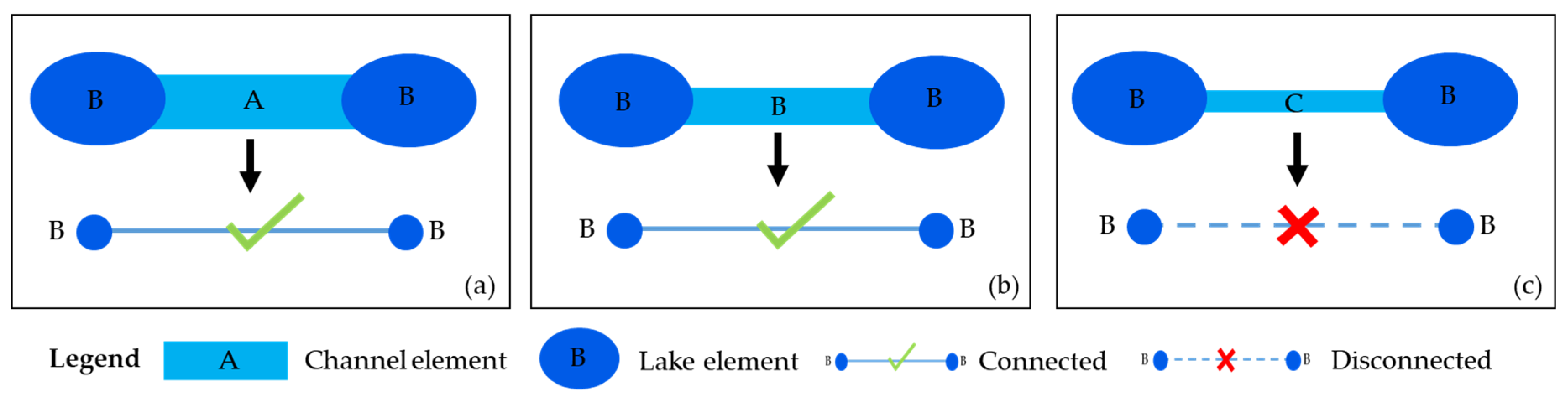
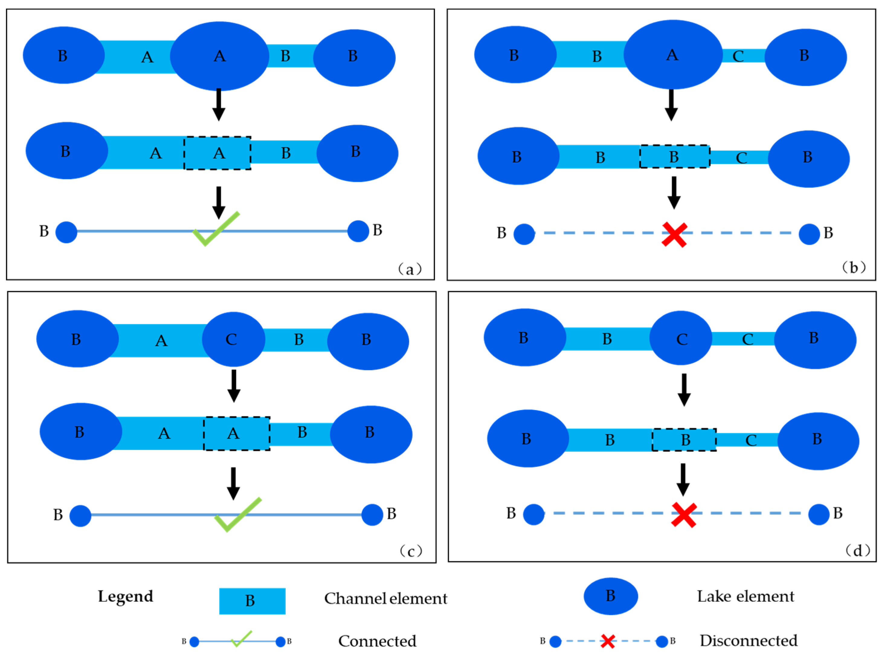
- Second, we identify and judge the simple connected form in the network—two lake elements are linked by the channel elements. In one grade network, if two lake elements of that grade are linked by the channel higher than that grade or of the same grade, the two lake elements are considered to be connected; on the contrary, if they are linked by the channel lower than this grade, it is judged as disconnected. For example, when a grade B network is formed, if two grade B lake elements are linked by a grade A or grade B channel, it is judged to be connected; if they are linked by a grade C channel it is judged as disconnected, see Figure 1. Check the entire network according to this rule.
- (3)
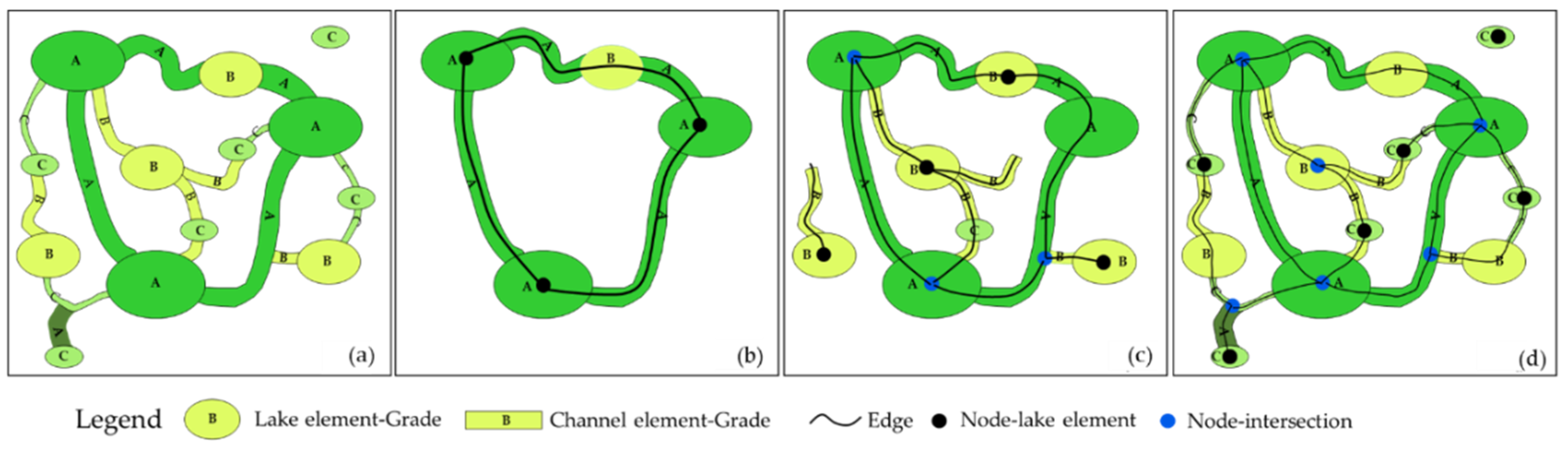
- Third, we identify and judge the complex connected form—two lake elements linked by a combination of channel and lake elements. When the grading forms the grade B network, the lakes and channels of grade B are the main body of the network. The complex connected form of grade B lake-channel-grade A or C lake-channel-grade B lake, the grade A or C lake should be transformed into the higher grade channel connected with it, and then we can judge whether two grade B lakes are connected or not by rule 2. For example, in Figure 2a, it is a complex connected form of grade B lake-grade A channel-grade A lake-grade B channel-grade B lake. To judge whether the two grade B lakes are connected, the grade A lake should be transformed into the grade A channel connected with it. Such a complex connected form becomes a simple connected form, that is, the grade B lake-grade A channel-grade A channel-grade B channel-grade B lake; two grade B lakes are connected by the high-grade channels, according to rule 2, and therefore the two grade B lakes are connected. In Figure 2b, the complex connected form of the grade B lake-grade B channel-grade A lake-grade C channel-grade B lake should be transformed into the simple connected form of the grade B lake-grade B channel-grade B channel-grade C channel-grade B lake. There are grade C channels in the connection, which indicates that the two grade B lakes are connected by low-grade channels, so they are disconnected. According to this rule, the various complex connected forms in the network can be judged, and finally the grading of the network can be completed.
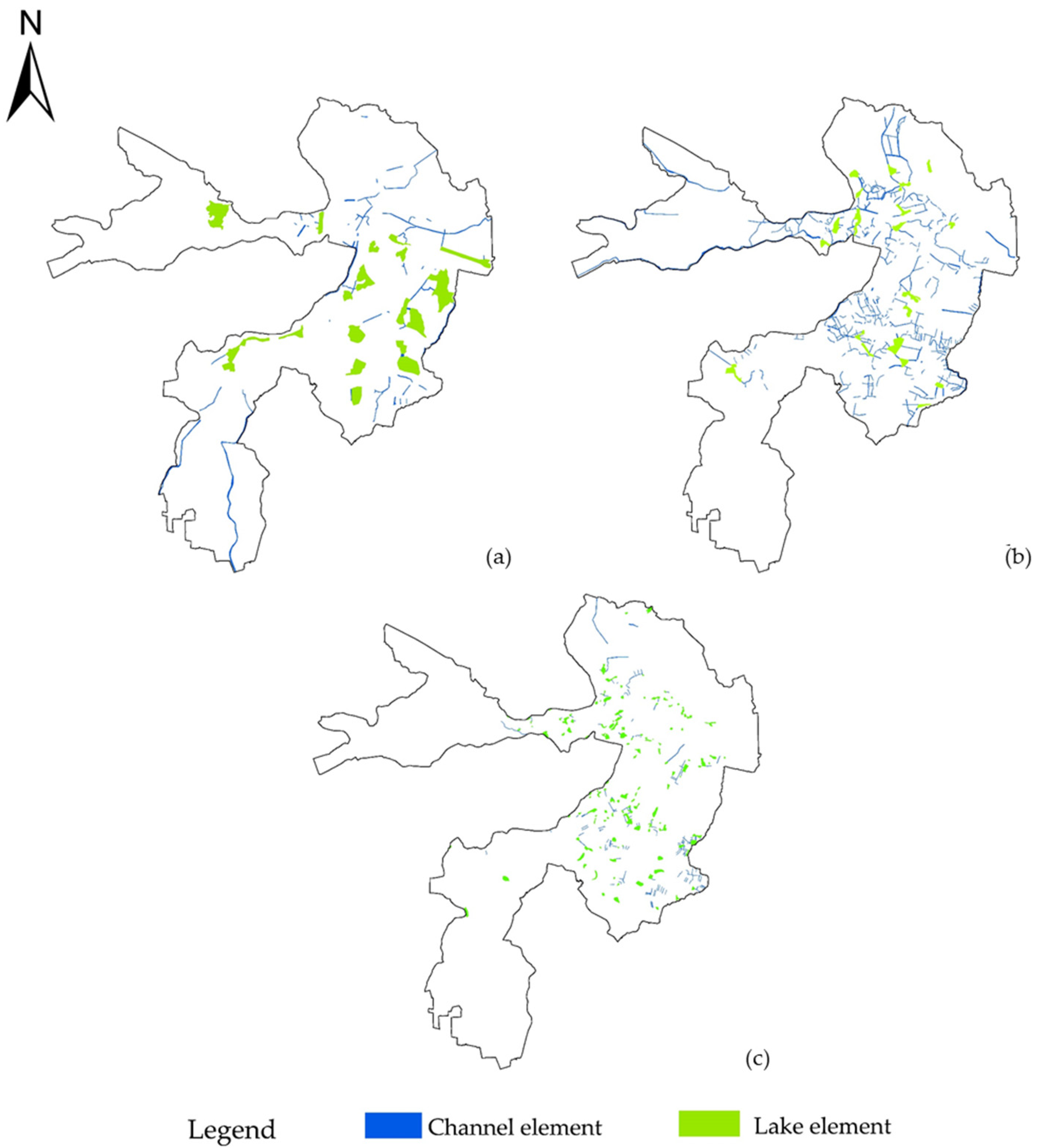
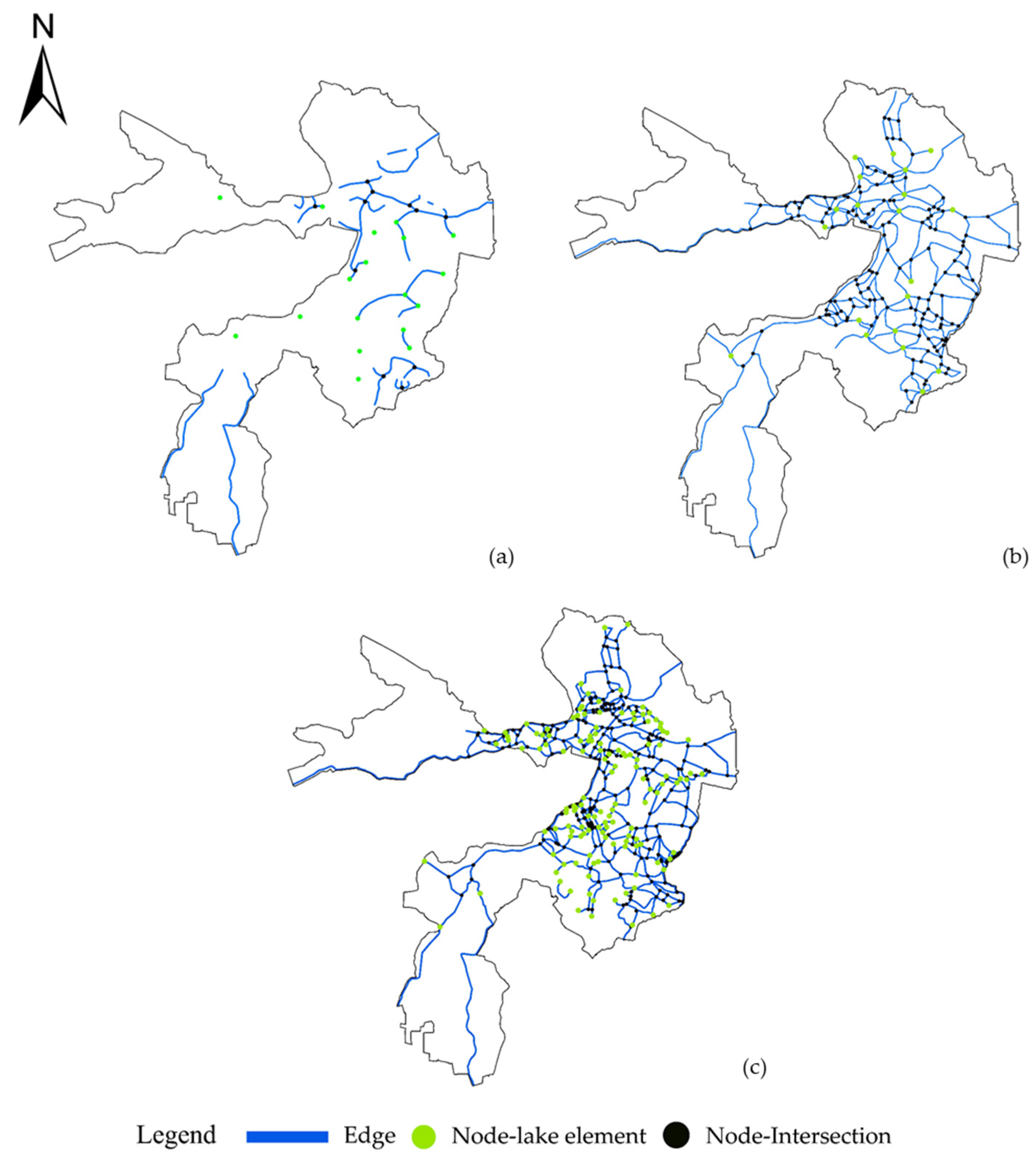
2.1.3. Extraction of Networks
2.2. Evaluation of Structural Connectivity
2.2.1. Development of the Indicator System
2.2.2. Weight Determination
- (1)
- Normalization
- (2)
- Index Entropy
- (3)
- Index Weightwhere: n denotes the number of indexes, m represents the number of evaluated objects, stands for the attribute value of the j-th index of the i-th evaluated object, represents the normalized value of the indicator, and refers to the entropy of the j-th index.
2.2.3. Structural Connectivity Index
3. Case Study
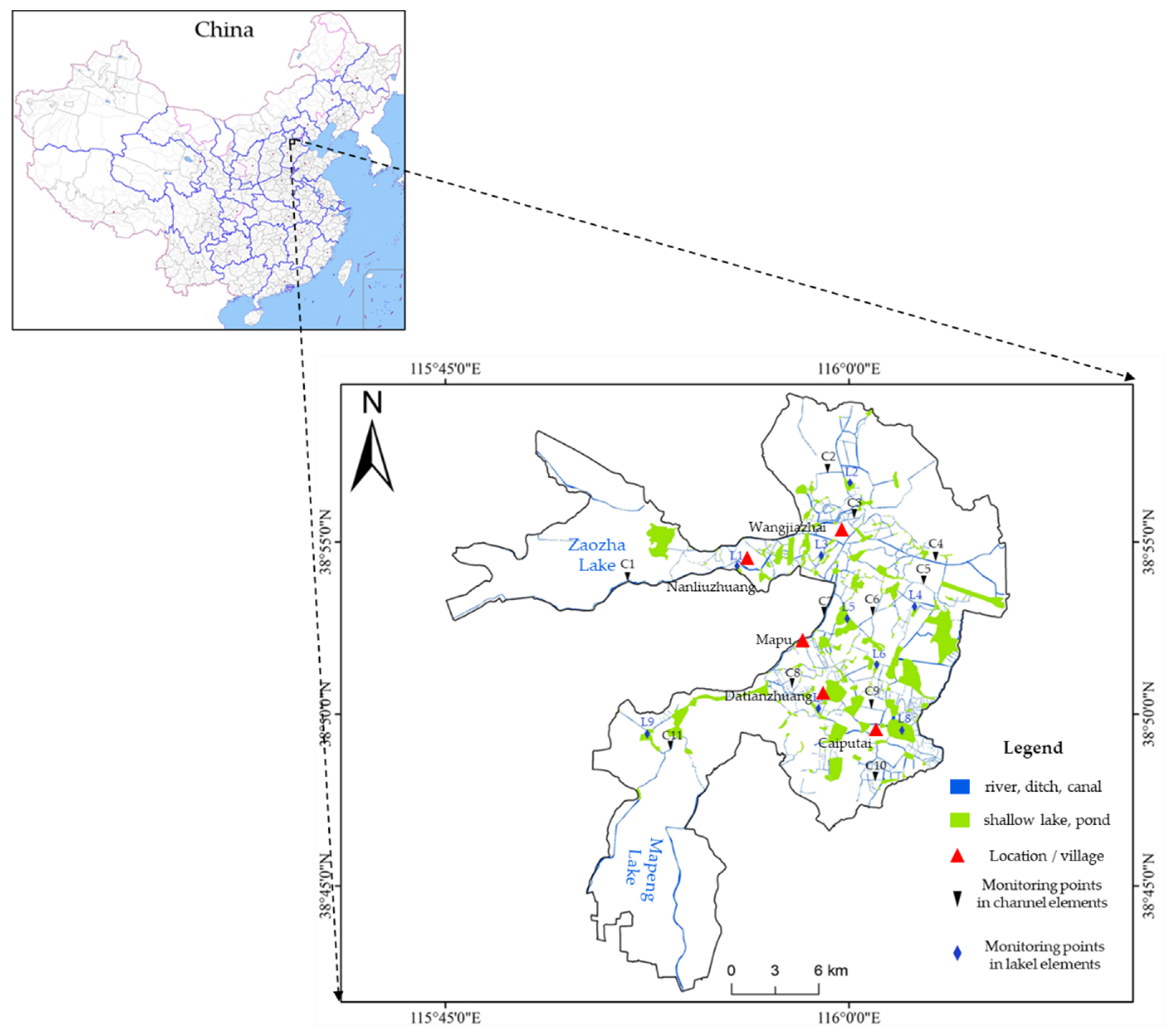
3.1. Study Area
3.2. Grading Results
3.2.1. Grading of Network Elements
3.2.2. Grading and Extraction of the Network
3.3. Evaluation of Structural Connectivity
3.3.1. Values and Weights of the Indicators
3.3.2. Connectivity Evaluation
4. Discussion
4.1. Comparison of Methods
4.2. Comparison of Results
4.3. Shortcomings of the Method
5. Conclusions
Author Contributions
Funding
Institutional Review Board Statement
Informed Consent Statement
Data Availability Statement
Acknowledgments
Conflicts of Interest
References
- Costanza, R.; d’Arge, R.; deGroot, R. The value of the world’s ecosystem services and natural capital. Nature 1997, 387, 253–260. [Google Scholar] [CrossRef]
- Alban, K.; Ant’onio, N.P.; Alvaro, S.-W.; María, D.B.; Luis, G. Ecological impacts of run-of-river hydropower plants—Current status and future prospects on the brink of energy transition. Renew. Sustain. Energy Rev. 2020, 142, 110833. [Google Scholar]
- Rogers, K.; Biggs, H. Integrating indicators, endpoints and value systems in strategic management of the rivers of the Kruger National Park. Freshw. Biol. 1999, 41, 439–451. [Google Scholar] [CrossRef]
- Shao, X.; Fang, Y.; Jawitz, J.W. River network connectivity and fish diversity. Sci. Total Environ. 2019, 689, 21–30. [Google Scholar] [CrossRef] [PubMed]
- Grill, G.; Lehner, B.; Lumsdon, A.E. An index-based framework for assessing patterns and trends in river fragmentation and flow regulation by global dams at multiple scales. Environ. Res. Lett. 2015, 10, 015001. [Google Scholar] [CrossRef]
- Suwal, N.; Kuriqi, A.; Huang, X.; Delgado, J.; Młyński, D.; Walega, A. Environmental Flows Assessment in Nepal: The Case of Kaligandaki River. Sustainability 2020, 12, 8766–8769. [Google Scholar] [CrossRef]
- Schiemer, F.; Hein, T.; Reckendorfer, W. Ecohydrology, key-concept for large river restoration. Ecohydrol. Hydrobiol. 2007, 7, 101–111. [Google Scholar] [CrossRef]
- Lesack, L.F.W.; Marsh, P. River-to-lake connectivities, water renewal, and aquatic habitat diversity in the Mackenzie River Delta. Water Resour. Res. 2010, 46, 45–53. [Google Scholar] [CrossRef]
- Meerkerk, A.L.; Wesemael, B.V.; Bellin, N. Application of connectivity theory to model the impact of terrace failure on runoff in semi-arid catchments. Hydrol. Proc. 2010, 23, 2792–2803. [Google Scholar] [CrossRef]
- Cui, B.; Wang, C.; Tao, W. River channel network design for drought and flood control: A case study of Xiaoqinghe River Basin, Jinan City, China. J. Environ. Manag. 2009, 90, 3675–3686. [Google Scholar] [CrossRef]
- Zhao, J.Y.; Dong, Z.R.; Zhai, Z.L. Evaluation method for river floodplain system connectivity based on graph theory. J. Hydraul. Eng. 2011, 42, 537–543. [Google Scholar]
- Bracken, L.J.; Croke, J. The concept of hydrological connectivity and its contribution to understanding runoff-dominated geomorphic systems. Hydrol. Proc. 2007, 21, 1749–1763. [Google Scholar] [CrossRef]
- Lane, S.N.; Reaney, S.M.; Heathwaite, A.L. Representation of landscape hydrological connectivity using a topographically driven surface flow index. Water Resour. Res. 2009, 45, 1–10. [Google Scholar] [CrossRef] [Green Version]
- Liu, X.; Zhang, Q.; Li, Y. Satellite image-based investigation of the seasonal variations in the hydrological connectivity of a large floodplain (Poyang Lake, China). J. Hydrol. 2020, 585, 124–141. [Google Scholar] [CrossRef]
- Shao, X.J.; Fang, Y.; Cui, B.S. A model to evaluate spatiotemporal variations of hydrological connectivity on a basin-scale complex river network with intensive human activity. Sci. Total Environ. 2020, 723, 138–153. [Google Scholar] [CrossRef]
- Chen, J.; Xiao, C.; Chen, D. Connectivity evaluation and planning of a river-lake system in east China based on graph theory. Math. Probl. Eng. 2018, 33, 31–42. [Google Scholar] [CrossRef]
- Chen, Y.; Wang, Y.G. Changes in river connectivity indexes in the lower Yellow River between 1960 and 2015. River Res. Appl. 2019, 35, 1377–1386. [Google Scholar] [CrossRef]
- Godsey, S.E.; Kirchner, J.W. Dynamic, discontinuous stream networks: Hydrologically driven variations in active drainage density, flowing channels and stream order. Hydrol. Proc. 2015, 28, 5791–5803. [Google Scholar] [CrossRef]
- Gao, C.J.; Gao, X.C.; Jia, P. Summary comments on hydrologic connectivity. Chin. J. Appl. Environ. Biol. 2017, 23, 586–594. [Google Scholar]
- Racchetti, E.; Bartoli, M.; Soana, E. Influence of hydrological connectivity of riverine wetlands on nitrogen removal via denitrification. Biogeochemistry 2011, 103, 335–354. [Google Scholar] [CrossRef]
- Xia, M.; Zhou, Z.; Zhao, H.X. Evaluation of water system connectivity of district around Chaohu Lake based on comprehensive index. Geo. Geo Inf. Sci. 2017, 33, 73–77. [Google Scholar]
- Detenbeck, N.E.; Elonen, C.M.; Taylor, D.L.; Anderson, T.M.; Jicha, S.L.; Batterman, S.L. Effects of hydrogeomorphic region, catchment storage and mature forest on baseflow and snowmelt stream water quality in second-order Lake Superior basin tributaries. Freshw. Biol. 2003, 48, 912–927. [Google Scholar] [CrossRef] [Green Version]
- Fullerton, A.H.; Burnett, K.M.; Steel, R.L.; Filtcroft, G.R.; Pess, B.E.; Feist, C.E. Hydrological connectivity for riverine fish: Measurement challenges and research opportunities. Freshw. Biol. 2010, 55, 2215–2237. [Google Scholar] [CrossRef] [Green Version]
- Keller, D.; Holderegger, R.; Van Strien, M.J. Spatial scale affects landscape genetic analysis of a wetland grasshopper. Mol. Ecol. 2013, 22, 2467–2482. [Google Scholar] [CrossRef]
- Zeug, S.C.; Winemiller, K.O. Relationships between hydrology, spatial heterogeneity, and fish recruitment dynamics in a temperate floodplain river. River Res. Appl. 2008, 24, 90–102. [Google Scholar] [CrossRef]
- Madenjian, C.P.; Bunnell, D.B. Depth distribution dynamics of the sculpin community in Lake Michigan. Trans. Am. Fish. Soc. 2008, 137, 1346–1357. [Google Scholar] [CrossRef]
- Xu, W.; Shen, Q.; Wang, X. Sensing images for assessing the minimum ecological flux by automatically extracting river surface width. Remote Sens. 2020, 12, 2899. [Google Scholar] [CrossRef]
- Liu, F.; Wang, J.L.; Fu, Z.S. Comparative research on effects of ecological ditches different in specification treating pollutants in drainage. Acta Pedol. Sin. 2019, 36, 562–569. [Google Scholar]
- Zheng, B.H.; Zhang, Y.; Li, Y.B. Study of indicators and method assessment of Liao River Basin. Acta Sci. Circum. 2007, 27, 928–936. [Google Scholar]
- Kail, J.; Brabec, K.; Poppe, M.; Januschke, K. The effect of river restoration on fish, macroinvertebrates and aquatic macrophytes: A meta-analysis. Ecol. Indic. 2015, 58, 311–321. [Google Scholar] [CrossRef]
- Feyrer, F.; Sommer, T.R.; Zeug, S.C.; O’Leary, G. Fish assemblages of perennial floodplain ponds of the Sacramento River, California (USA) with implications for the conservation of native fishes. Fish. Manag. Ecol. 2004, 24, 335–344. [Google Scholar] [CrossRef]
- Roozen, F.C.J.M.; Van Geest, G.J.; Ibelings, B.W. Lake age and water level affect the turbidity of floodplain lakes along the lower Rhine. Freshw. Biol. 2003, 48, 519–531. [Google Scholar] [CrossRef]
- Miranda, L.E. Depth as an organizer of fish assemblages in floodplain lakes. Aquat. Sci. 2011, 73, 211–221. [Google Scholar] [CrossRef]
- Cohen, M.J.; Brown, M.T. A model examining hierarchical wetland networks for watershed stormwater management. Ecol. Model. 2007, 201, 179–193. [Google Scholar] [CrossRef]
- Sun, C.; Knig, H.J.; Sanda, U.; Cheng, C.; Karoline, H. Protection effect of overwintering water bird habitat and defining the conservation priority area in Poyang Lake wetland, China. Environ. Res. Lett. 2020, 15, 125013. [Google Scholar] [CrossRef]
- Dodson, S. Predicting crustacean zooplankton species richnes. Limnol. Oceanogr. 1992, 37, 123–131. [Google Scholar] [CrossRef]
- Gao, T.; Yin, X.A.; He, S.; Zhao, Y.W. Structural connectivity evaluation of Baiyangdian water system. J. Hydrol. 2020, 41, 63–69. [Google Scholar]
- Xu, G.L.; Xu, Y.P.; Wang, L.Y. Evaluation of river network connectivity based on hydraulic resistance and graph theory. Adv. Water Sci 2012, 23, 776–781. [Google Scholar]
- Saaty, T.L. The Analytic Hierarchy Process: Planning, Priority Setting; McGraw-Hill: New York, NY, USA, 1980. [Google Scholar]
- Delgado, A.; Romero, I. Environmental conflict analysis using an integrated grey clustering and entropy-weight method: A case study of a mining project in Peru. Environ. Model. Softw. 2016, 77, 108–121. [Google Scholar] [CrossRef]
- Miranda, L.E.; Killgore, K.J. Fish depth distributions in the Lower Mississippi River. River Res. Appl. 2014, 30, 347–359. [Google Scholar] [CrossRef]
- Xie, S.; He, H.D. Present condition analysis of Hebei Baiyangdian lake fish stocks after diversion from Yellow River to the lake. Sci. Tech. Inform. 2010, 23, 433–436. [Google Scholar]
- Wang, Y.H.; Wu, T.T.; Fan, J.G. Hou Jianhua Avian community and group diversity of Baiyangdian Lake in summer. J. Hebei Univ. Nat. Sci. Ed. 2018, 38, 443–448. [Google Scholar]
- Du, H.; Ban, X.; Zhang, H.; Wei, Q.W.; Chen, D.Q. Preliminary observation on preference of fish in natural channel to water depth and velocity—A case study of the Yangtze River from Jiang Kou town to Yuan Shi town. J. Yangtze River Sci. Res. Inst. 2010, 27, 70–74. [Google Scholar]
- Gilbert, G.; Tyler, G.A.; Dunn, C.J.; Smith, K.W. Nesting habitat selection by bitterns Botaurus stellaris in Britain and the implications for wetland management. Biol. Conserv. 2005, 124, 547–553. [Google Scholar] [CrossRef]
- China Biodiversity Conservation and Green Development Foundation. Rapid Assessment in Research of Wild Fish Resource in Baiyangdian Wetland and Sustainable Utilization; CBCGDF: BaoDing, China, 2017. [Google Scholar]
- Zhao, Z.X. Coupling Mechanism of Eco-Hydrological Processes and Integrated Regulation in Baiyangdian Wetland. Ph.D. Thesis, Tianjin University, Tianjin, China, 2012. [Google Scholar]
- Wu, M.L. The Study on Structure and Diversity of Bird Communities in the Baiyangdian Wetland of Hebei Province Hebei; Hebei Wildlife Protection Association: Shijiazhuang, China, 2007; pp. 70–78. [Google Scholar]
- Yan, X.; Niu, Z.G. Spatial-temporal Variation Characteristics of Baiyangdian from 1990 to 2017. Chin. J. Wet. Sci. 2019, 17, 436–444. [Google Scholar]


| Name | Connotation | Relationship between Structural and Functions | Acquisition and Application |
|---|---|---|---|
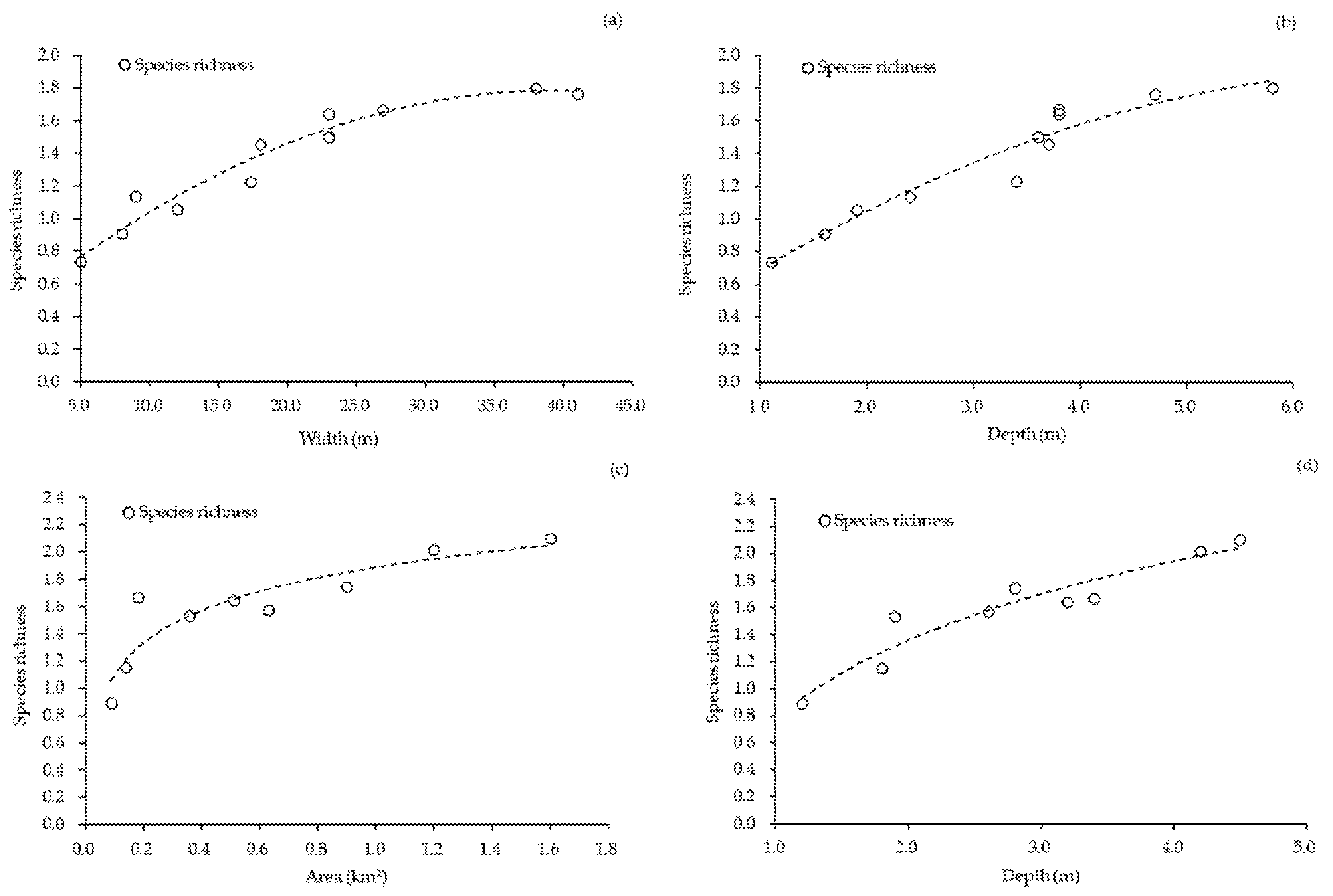
| Width | The structural width of channel elements such as rivers, canals, and ditches. | There is a relationship between the width, water level, and water flow of a river, with the minimum width corresponding to the minimum ecological flow and water level [27]. The width of a ditch affects its pollutant removal efficiency [28]. River width is one of the important indicators to evaluate the suitability of fish habitat, which is directly related to fish biodiversity [29]. River size affected the effect on fish abundance/biomass increased with river width [30]. | The data is obtained through high-precision remote sensing image measurement or on-site surveying and mapping. According to the relationship between width and function, the standard of element grading is established, that is, the width threshold corresponding to different grade channel elements. When the channel width belongs to which threshold, the channel should be divided into the grade A or B or C *. |
| Depth | The structural depth of channel elements such as rivers, canals, and ditches. The average structural depth of lake elements such as shallow lakes and ponds. | Habitat-specific factors such as hydrology, depth, turbidity and geomorphology significantly influence the species composition and abundance in river systems [31]. Phytoplankton biomass was influenced by the lake properties, depth, and floating vegetation [32]. Depth is a causal factor that drives many physical and chemical variables that contribute to organizing fish assemblages in shallow lakes. [33]. | The data needs to be obtained through measured terrain data. By analyzing the relationship between the channel depth and the ecological or environmental function, the standard of element grading is established, that is, the depth threshold corresponding to different grade elements. When the channel depth belongs to which threshold, the channel should be divided into the grade A or B or C *. |
| Area | The area of lake elements such as shallow lakes and ponds. | Area directly affects the wetland’s contribution in removing pollutants [34]. Lake area is an important index to evaluate waterfowl habitat, which is directly related to their survival and biodiversity, especially in shallow lake wetlands [35]. Zooplankton species richness often increases as a linear function of lake area, possibly because habitat diversity increases with lake size [36]. | The data is obtained through high-precision remote sensing image measurement or on-site surveying and mapping. By analyzing the relationship between the lake element area and the ecological or environmental function, the standard of element grading is established, that is, the area threshold corresponding to different grade elements. When the lake area belongs to which threshold, the lake should be divided into the grade A or B or C *. |
| Order | Layers | Indicators | Definition | Equation | Unit |
|---|---|---|---|---|---|
| 1 | Layout of the network | Density of lake elements (LD) | The area of lake elements per unit area | where LA denotes the area covered by lake elements and A represents the total study area. | Dimensionless |
| 2 | Frequency of channel elements (Cf) | The number of channel elements per unit area | where CN refers to the number of channel elements and A represents the total study area. | km−2 | |
| 3 | Connectivity of the network | Loop ratio of network (α) | The ratio of the actual number of loops to the maximum number of possible loops in the network, which reflects the material and energy exchange capacity of a node. | where E denotes the number of edges and N is the number of nodes. | Dimensionless |
| 4 | Node connection rate (β) | How easy it is for each node to connect to other nodes. | where E denotes the number of edges and N is the number of nodes. | Dimensionless | |
| 5 | Edge connectivity ratio (CP) | The ratio of the number of connected node pairs to the total number of node pairs, which reveals the connectivity of edges from the number of connected nodes. | where CNp denotes the number of connected node pairs and Np denotes the total number of node pairs. | Dimensionless | |
| 6 | Network connectedness (γ) | The ratio of the number of connected channels to the maximum number of possibly connected channels. | (N ≥ 3) where E denotes the number of edges, N denotes the number of nodes, and Lmax represents the maximum number of edges that are possibly connected. | Dimensionless | |
| 7 | Smoothness of the network | Smoothness of water flow (ω) | The unobstructed degree of water flow, which equals the reciprocal of the resistance to water flow. | where b denotes bottom width of the channel element, h is the depth of the channel element, and m represents the slope coefficient. | Dimensionless |
| Monitoring Points | Structural Attributes | Species Richness | |
|---|---|---|---|
| Width | Depth | ||
| C1 | 26.9 | 3.8 | 1.67 |
| C2 | 12 | 1.9 | 1.06 |
| C3 | 8 | 1.6 | 0.91 |
| C4 | 38 | 5.8 | 1.80 |
| C5 | 17.3 | 3.4 | 1.23 |
| C6 | 23 | 3.8 | 1.64 |
| C7 | 41 | 4.7 | 1.76 |
| C8 | 5 | 1.1 | 0.74 |
| C9 | 18 | 3.7 | 1.46 |
| C10 | 9 | 2.4 | 1.14 |
| C11 | 23 | 3.6 | 1.50 |
| Monitoring Points | Structural Attributes | Species Richness | |
|---|---|---|---|
| Area | Depth | ||
| L1 | 0.14 | 1.8 | 1.15 |
| L2 | 0.63 | 2.6 | 1.57 |
| L3 | 0.09 | 1.2 | 0.89 |
| L4 | 0.18 | 3.4 | 1.67 |
| L5 | 1.2 | 4.2 | 2.02 |
| L6 | 0.36 | 1.9 | 1.53 |
| L7 | 0.51 | 3.2 | 1.64 |
| L8 | 1.6 | 4.5 | 2.10 |
| L9 | 0.9 | 2.8 | 1.75 |
| Monitoring Points | Species | |||||||
|---|---|---|---|---|---|---|---|---|
| Carassius auratus | Cyprinus carpi | Pseudobagrus fulvidraco | Hypophthalmichthys molitrix | Ctenopharyngodon idellus | Silurus asotus | Hemiculter leucisculus | Pseudorasbora parva | |
| C1 | 0.11 | 0.26 | 0.10 | 0.28 | 0.00 | 0.00 | 0.38 | 0.33 |
| C2 | 0.38 | 0.00 | 0.00 | 0.29 | 0.00 | 0.00 | 0.77 | 0.41 |
| C3 | 0.23 | 0.00 | 0.00 | 0.00 | 0.00 | 0.13 | 0.78 | 0.69 |
| C4 | 0.17 | 0.31 | 0.03 | 0.24 | 0.18 | 0.00 | 0.22 | 0.00 |
| C5 | 0.10 | 0.15 | 0.00 | 0.38 | 0.00 | 0.00 | 0.46 | 0.58 |
| C6 | 0.18 | 0.26 | 0.00 | 0.12 | 0.00 | 0.17 | 0.40 | 0.30 |
| C7 | 0.13 | 0.21 | 0.05 | 0.27 | 0.23 | 0.00 | 0.21 | 0.08 |
| C8 | 0.00 | 0.00 | 0.00 | 0.00 | 0.00 | 0.21 | 0.98 | 0.57 |
| C9 | 0.19 | 0.00 | 0.11 | 0.38 | 0.06 | 0.00 | 0.44 | 0.41 |
| C10 | 0.31 | 0.00 | 0.00 | 0.00 | 0.00 | 0.31 | 0.48 | 0.50 |
| C11 | 0.36 | 0.00 | 0.06 | 0.22 | 0.14 | 0.00 | 0.44 | 0.36 |
| Monitoring Points | Species | |||||||||
|---|---|---|---|---|---|---|---|---|---|---|
| Carassius auratus | Cyprinus carpi | Pseudobagrus fulvidraco | Hypophthalmichthys molitrix | Ctenopharyngodon idellus | Megalobrama amblycephala | Silurus asotus | Hemiculter leucisculus | Pseudorasbora parva | Abbottina rovularis | |
| L1 | 0.27 | 0.00 | 0.00 | 0.24 | 0.00 | 0.00 | 0.00 | 0.33 | 0.76 | 0.02 |
| L2 | 0.11 | 0.40 | 0.00 | 0.35 | 0.00 | 0.04 | 0.00 | 0.77 | 0.00 | 0.00 |
| L4 | 0.16 | 0.22 | 0.00 | 0.00 | 0.00 | 0.00 | 0.00 | 0.55 | 0.68 | 0.01 |
| L3 | 0.13 | 0.13 | 0.00 | 0.25 | 0.00 | 0.00 | 0.04 | 0.72 | 0.18 | 0.00 |
| L5 | 0.24 | 0.04 | 0.04 | 0.45 | 0.22 | 0.03 | 0.00 | 0.12 | 0.21 | 0.00 |
| L6 | 0.36 | 0.00 | 0.00 | 0.21 | 0.12 | 0.00 | 0.00 | 0.65 | 0.31 | 0.00 |
| L7 | 0.11 | 0.28 | 0.00 | 0.55 | 0.00 | 0.00 | 0.00 | 0.22 | 0.52 | 0.00 |
| L8 | 0.40 | 0.20 | 0.00 | 0.43 | 0.14 | 0.02 | 0.00 | 0.00 | 0.36 | 0.00 |
| L9 | 0.12 | 0.27 | 0.02 | 0.35 | 0.15 | 0.00 | 0.00 | 0.38 | 0.22 | 0.00 |
| Channel Element Grade | Width w (m) | Water Depth d (m) |
|---|---|---|
| Large | w ≥ 25 | d ≥ 4 |
| Medium | 10 ≤ w < 25 | 2 ≤ d |
| w ≥ 25 | d < 4 | |
| Small | 10 < w | 0 < d |
| 10 ≤ w < 25 | d < 2 |
| Lake Element Grade | Area a (km2) | Water Depth d (m) |
|---|---|---|
| Large | a ≥ 0.5 | d ≥ 4 |
| Medium | 0.2 ≤ a < 0.5 | 2 ≤ d |
| a ≥ 0.5 | d < 4 | |
| Small | a < 0.2 | 0 < d |
| 0.2 ≤ a < 0.5 | d < 2 |
| Channel Element Grade | Quantity (No. of Elements) | Lake Element Grade | Quantity (No. of Elements) |
|---|---|---|---|
| Large | 67 | Large | 17 |
| Medium | 369 | Medium | 20 |
| Small | 162 | Small | 136 |
| Total | 598 | Total | 173 |
| Network Grade | Edges (No.) | Nodes-Lake Element (No.) | Node-Intersection (No.) |
|---|---|---|---|
| Large | 39 | 17 | 11 |
| Medium | 267 | 20 | 144 |
| Small | 534 | 136 | 231 |
| Order | Indicators (Unit) | Network Size | Weight | ||
|---|---|---|---|---|---|
| Large | Medium | Small | |||
| 1 | LD (dimensionless) | 0.077 | 0.024 | 0.021 | 0.094 |
| 2 | Cf (km−2) | 0.193 | 1.063 | 0.467 | 0.094 |
| 3 | α (dimensionless) | 0.090 | 0.322 | 0.230 | 0.208 |
| 4 | β (dimensionless) | 2.690 | 3.256 | 2.910 | 0.114 |
| 5 | CP (dimensionless) | 0.569 | 0.964 | 0.889 | 0.107 |
| 6 | γ (dimensionless) | 0.350 | 0.549 | 0.485 | 0.130 |
| 7 | ω (dimensionless) | 0.320 | 0.710 | 0.530 | 0.253 |
Publisher’s Note: MDPI stays neutral with regard to jurisdictional claims in published maps and institutional affiliations. |
© 2021 by the authors. Licensee MDPI, Basel, Switzerland. This article is an open access article distributed under the terms and conditions of the Creative Commons Attribution (CC BY) license (https://creativecommons.org/licenses/by/4.0/).
Share and Cite
Tian, K.; Yin, X.-a.; Bai, J.; Yang, W.; Zhao, Y.-w. Grading Evaluation of the Structural Connectivity of River System Networks Based on Ecological Functions, and a Case Study of the Baiyangdian Wetland, China. Water 2021, 13, 1775. https://doi.org/10.3390/w13131775
Tian K, Yin X-a, Bai J, Yang W, Zhao Y-w. Grading Evaluation of the Structural Connectivity of River System Networks Based on Ecological Functions, and a Case Study of the Baiyangdian Wetland, China. Water. 2021; 13(13):1775. https://doi.org/10.3390/w13131775
Chicago/Turabian StyleTian, Kai, Xin-an Yin, Jie Bai, Wei Yang, and Yan-wei Zhao. 2021. "Grading Evaluation of the Structural Connectivity of River System Networks Based on Ecological Functions, and a Case Study of the Baiyangdian Wetland, China" Water 13, no. 13: 1775. https://doi.org/10.3390/w13131775
APA StyleTian, K., Yin, X.-a., Bai, J., Yang, W., & Zhao, Y.-w. (2021). Grading Evaluation of the Structural Connectivity of River System Networks Based on Ecological Functions, and a Case Study of the Baiyangdian Wetland, China. Water, 13(13), 1775. https://doi.org/10.3390/w13131775