Effects of Decaying Hydraulic Conductivity on the Groundwater Flow Processes in a Managed Aquifer Recharge Area in an Alluvial Fan

Abstract

Groundwater artificial recharge and medium characteristics represent the major factors in controlling the groundwater flow processes in managed aquifer recharge areas. According to the depositional features of alluvial fans, an analogous homogeneous phreatic sand tank aquifer and the corresponding inhomogeneous scale numerical models were established to investigate the groundwater flow under the combined influence of artificial recharge (human activities) and decaying hydraulic conductivity (medium characteristics). In this study, groundwater flow through a managed aquifer recharge area in an alluvial fan was analyzed under the conditions of decaying hydraulic conductivity (K) with depth or length from apex to apron. The results showed that groundwater flow processes induced by artificial recharge were significantly controlled by the increasing decay exponents of K. The decaying K with depth or length in alluvial fan areas expanded the degree of influence of artificial recharge on groundwater flow. With the increase of decay exponents, the flow directions gradually changed from a horizontal to vertical direction. Groundwater age and spatial variability could also be increased by the increasing decay exponents. The residence time distributions (RTDs) of ambient groundwater and artificially recharged water exhibited logarithmic, exponential, and power law behavior. Penetration depth and travel times of ambient groundwater flow could be affected by artificial recharge and decay exponents. Furthermore, with the increase of decay exponents, the thickness of the artificially recharged water lens and travel times of artificially recharged water were increased. These findings have important implications for the performance of managed aquifer recharge in alluvial fan areas as well as the importance of considering the gradual decrease of K with depth and length.

1. Introduction

Alluvial fans are becoming an important area of interest for groundwater artificial recharge [1,2,3,4,5] given their substantial thickness, high porosity, huge storage capacity [6], and abundant groundwater resources such as those in Northwest China [7] and Hueco Bolson in the United States and Mexico [8]. In most of the alluvial fans, excessive groundwater withdrawal to meet increasing demand for water resources because of population increase and economic growth has resulted in water table decline, land subsidence, and saltwater intrusion [9,10,11]. Groundwater artificial recharge is an important method of ensuring sustainability of water resources on a local or regional scale in alluvial fans [7,12,13,14]. Previous studies showed that groundwater flow features, such as moisture content, groundwater flow patterns, groundwater age, RTDs, and groundwater flow paths, are significantly influenced by artificial recharge [15].

Alluvial fans are generally defined as semi-conical depositional landforms along mountain piedmonts [16], which have a morphology that consists of three main parts from apex to apron: inner fan (short extension and coarse granulometry of deposits), mid fan (smaller grain-size of particles and bedded deposits), and outer fan (largest area made by fine-grained bedded deposits) [17]. These features (the particle size decreases gradually from coarse to fine from apex to apron) reflect the facies architecture developed during their evolution and formed due to the change of hydrodynamic conditions [17,18,19]. As observed previously, the particle size of fans normally reflects the permeability of the sediment, and many empirical formulas have been founded based on the relationship between particle size and K [20,21]. The coarser particle size, the larger the K. For example, K of the alluvial fan aquifer in the northwest of the Hetao basin decreases from 2.0 m/d along the mountain front to 0.2 m/d in the downdip region [22].

Controlled by development patterns and geometric features of fractures [23], regional metamorphism [24], and particle size, and so on, existing studies using statistical methods such as histograms and semi-variograms have shown that the K typically follows a normal distribution [25], log-normal distribution [23,26,27], or a Levy stable distribution [28]. Besides particle size, K of aquifers could be affected by some other geological factors [24], such as in situ stress conditions [29,30], weathering, and unloading processes [31]. Thus, K was commonly found to vary spatially with depth [32,33]. Regression analysis has also been used to study the statistical distribution of K in different sites and has shown that the variation of K with depth could be described by different functions, such as power function [23], logistic function [23], and exponential function [33]. The systematic decrease in K with depth has been proven to affect various features of subsurface flow such as the flow paths, velocity, travel times, and RTDs [20,34,35,36,37].

Groundwater flow features are critical for understanding the variety of groundwater flow systems, which is essential for protecting regional water supply security, facilitating environmental conservation and water resources management [38,39,40]. The effects of human activities on groundwater flow features, such as groundwater pumping, artificial recharge, and urbanization, have been studied in recent research [15,41,42,43]. Many other investigations, including field studies and numerical simulations, have been carried out to examine the pattern of groundwater flow under the depth-decaying K, showing that regional flow systems, solute transport, flow paths, and RTDs are sensitive to the depth-decaying behavior of K [20,34,35,36,37,44]. While these studies generated important insights into the groundwater flow behavior under depth-decaying K or human activities, none of them considered the effects of systematic decrease in K along the length from the apex to apron (length-dependent hydraulic conductivity) on groundwater flow in alluvial fan areas and the combined effects of artificial recharge and decaying K, which have been widely observed in geological formations because of the specific depositional environment.

The aim of this study was to develop a sand tank model and conduct numerical modeling to investigate groundwater flow in an alluvial area affected by artificial recharge and decaying K in different directions. The results represent an advance over the usual limitations of zonal heterogeneity and layered heterogeneity of hydraulic conductivity applied in groundwater flow modeling and provide insights into the groundwater flow affected by artificial recharge and medium characteristics. The results have some practical implications for ecological environment protection, sustainable water resource evaluation, and aquifer management in similar areas.

2. Methodology

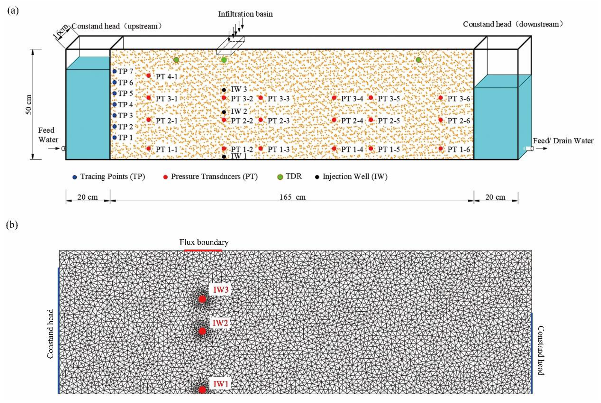
2.1. Laboratory Experiments

An acrylic glass tank measuring 2.05 (length) × 0.5 (height) × 0.16 m (width) was carried out to simulate a two-dimensional cross-section of a homogeneous phreatic aquifer and used for laboratory experiments (Figure 1a). The general setup of the laboratory experiments was adopted from Atlabachew et al. [45] and Wu et al. [15]. However, the sand tank was only used for the homogeneous scenario here. Computer-controlled pumps were connected to three injection wells (IW 1–3). In total, 19 high-sensitivity deflated pressure transducers (PTs) (HM20-1-A1-F2-W2, by German HELM) were buried directly into the back face of the sand tank to measure hydraulic pressure. The saturated hydraulic conductivity of the sand was 40 m/d as measured using the constant-head method, and the bulk porosity was found to be 0.3 using the oven-drying method (Chinese National Standard). Detailed descriptions of the filter sands and the methods employed for the determination of their particle size can be found in Wu et al. [15].

It is important to point out that the sand tank experiments acted as the foundation of the following numerical model. That is, the sand tank experiments had neutral conditions with non-decaying hydraulic conductivity. The sand tank experiments could also show phenomena that actually occurred in the artificially recharged aquifer, for example, the flow field above the water table.

2.2. Numerical Simulation

Exploration into the roles of hydrodynamics (surface and subsurface) based on an actual research area requires detailed geomorphological and hydrogeological data, which are rarely available [46], so a synthetic model is always needed for solving such problems. In this study, a theoretical groundwater flow model generalized from an alluvial fan was constructed to explore the role of the artificial recharge and decaying K in controlling the groundwater flow by using the finite element model FEFLOW, which is a variably saturated groundwater flow modeling program. The homogeneous numerical model was constructed according to the sand tank and adjected slightly. Then, the numerical models with decaying K were expanded based on the homogeneous one. The finite element mesh and boundary conditions for the numerical solution are shown in Figure 1b.

The basic equation describing the groundwater flow simulated in the FEFLOW code is shown below.

$${\mathit{s}\mathit{S}}_0\frac{\mathit{\partial }\mathit{h}}{\mathit{\partial }\mathit{t}}+\mathit{\epsilon }\frac{\mathit{\partial }\mathit{s}}{\mathit{\partial }\mathit{t}}+\nabla {\times \mathbf{q}=\mathit{Q}+\mathit{Q}}_{\mathrm{EOB}}$$

(1)

$${\mathbf{q}=-\mathit{k}}_{\mathit{r}}{\mathbf{K}\mathit{f}}_{\mathit{\mu }}\times (\nabla \mathit{h}+\chi \mathit{e})$$

(2)

where s is the saturation of fluid in the void space$\mathit{\epsilon }$ [1], ${\mathit{S}}_0$ is the specific storage coefficient [L⁻¹], h is the hydraulic head [L], t is time [T], $\mathit{\epsilon }$ is the porosity (void space) [1], $\mathrm{\nabla }$ is the Nabla (vector) operator [L⁻¹], q is the Darcy velocity of fluid [L T⁻¹], Q is the bulk source/sink term of flow [L³ T⁻¹], Q_EOB is the correction sink/source term of the extended Oberbeck–Boussinesq approximation [T⁻¹], ${\mathit{k}}_{\mathit{r}}$ is the relative permeability [1], K is the tensor of hydraulic conductivity [LT⁻¹], ${\mathit{f}}_{\mathit{\mu }}$ is the viscosity relation function [1], $\mathit{\chi }$ is the buoyancy coefficient [1], and e is the gravitational unit vector [1].

The nonlinear depth-dependent K (z) was described by using the exponential decay model [35,36]. Assuming a locally isotropic condition, the depth-dependent K (z) is given by:

$$\mathbf{K}\left(\mathrm{z}\right){=\mathbf{K}}_0{\exp [-\mathrm{A}}_1{(\mathrm{z}}_{\mathrm{s}}\left(\mathrm{x}\right)-\mathrm{z}\left)\right]$$

(3)

where K₀ is the K at the ground surface. The K₀ adopted in the numerical model was the same as that measured in the sand tank. A₁ is the decay exponent that dictates the rate of decrease in K with depth, z_s(x) is a function of the ground surface elevation, and z is the elevation of the aquifer bottom.

There is a lack of relevant research on the variation law of K with the length from apex to apron zone, which approximately follows an exponential law in the Tailan river basin (Figure 2). The main purpose of this study was to investigate how the decaying hydraulic conductivity affects the groundwater flow; a further precise study on the variation law was not conducted here, and the length-dependent K(x) was assumed to be:

$$\mathbf{K}\left(\mathbf{x}\right){=\mathbf{K}}_0{\exp [-\mathrm{A}}_2{(\mathrm{x}}_{\mathrm{u}}\left(\mathrm{z}\right)-\mathrm{x}\left)\right]$$

(4)

where A₂ is the decay exponent that dictates the rate of decrease in K with length, and x_u(z) is a function of the vertical boundary on the upper reaches side.

2.3. Scenario Definition

Three scenarios (scenarios A–C) were conducted to mimic the groundwater flow induced by artificial recharge and decaying K. Scenario A was conducted in the sand tank aquifer and corresponding numerical model and represents the condition of artificial recharge in a homogeneous phreatic aquifer. The water levels were controlled at 43 and 25 cm above the inner base of the tank at the entrance (left) and exit (right) water chambers, respectively. The flow fields were measured in the steady-state condition.

Scenario B was conducted using a numerical model, based on the homogeneous one corresponding to sand tank experiment, with artificial recharge at different locations (infiltration basin and injection wells at different depths of the lab-scale aquifer) and decaying K with depth. Various decay exponents with depth (A₁) have been reported in the literature, mostly ranging from 0.003 to 0.5 [20,33,35,36]. Here, we set the decay exponents as 0.01, 0.05, and 0.1 m⁻¹. The corresponding K fields and their relationships to depth are shown in Figure 3 and Figure 4, respectively. The artificial recharge rate through the infiltration basin was set to 5 and 0.2 m/d in the injection wells. The water level in the right and left water chambers was the same as that in scenario A.

Scenario C was also conducted with a numerical model, with artificial recharge at different locations and decaying K with length from apex to apron zone. Various decay exponents along the length from the apex to apron are not reported. For the main purpose of investigating the response of artificially recharged groundwater flow to the decay of K along the length direction, the A₂ was assumed as 0.005, 0.01, and 0.02 m⁻¹ here. The corresponding K fields and their relationships with length are shown in Figure 5 and Figure 6, respectively. The artificial recharge rate and water level in the water chambers were the same as those in scenario B.

3. Results

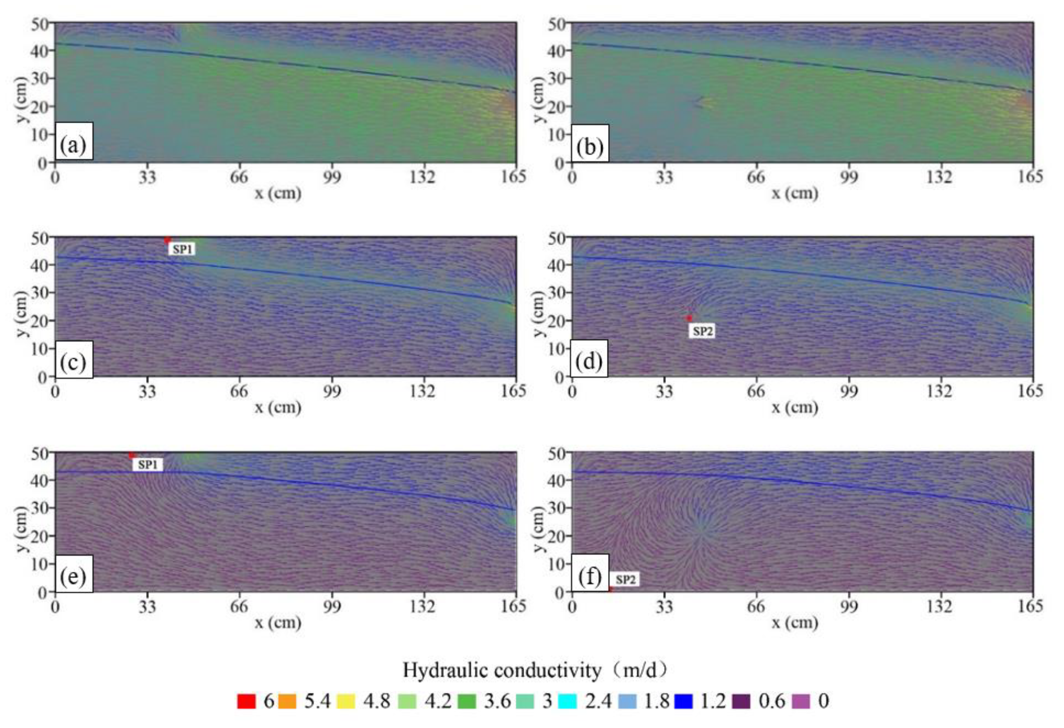
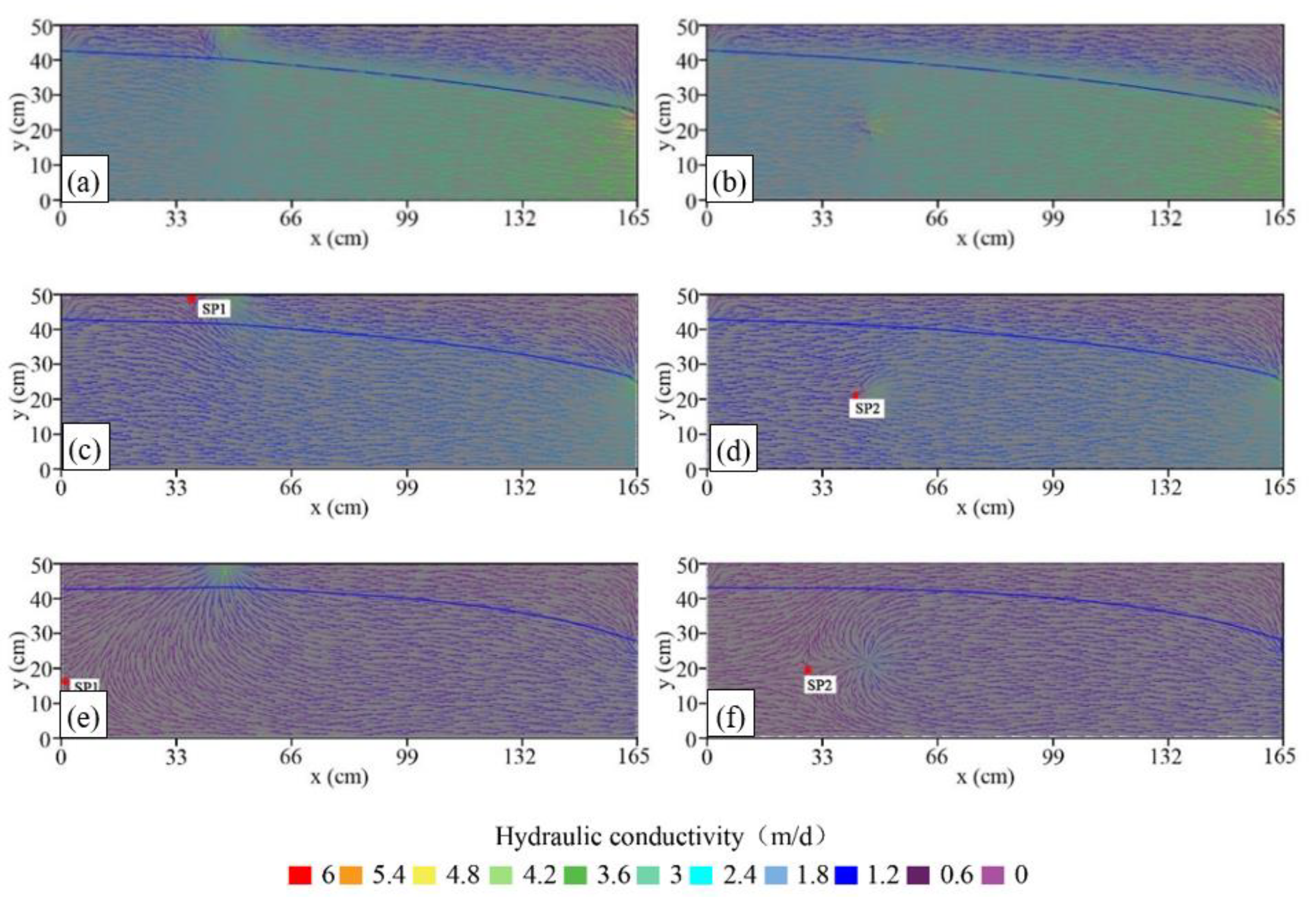
3.1. Groundwater Flow Patterns

Groundwater flow patterns induced by different depth- and length-decay exponents and artificial recharge (artificial recharge through the infiltration basin and injection well IW3 were taken as examples here) are shown in Figure 7 and Figure 8, respectively. Figure 7a,b and Figure 8a,b showed that the smaller artificial recharge rate (the artificial recharge rate in infiltration basin is 5 and 0.2 m/d in injection well IW3) did not affect the flow fields obviously when the decay exponents were smaller (when the depth-decay exponent was 0.01 m⁻¹ and length-decay exponent was 0.005 m⁻¹). The flow directions were almost horizontal from upstream to downstream direction. The velocities ranged from 3 to 4.2 m/d and increased along the flow paths. The left-side and right-side figures in Figure 7 and Figure 8 also show that the velocities decreased with the increase of decay exponents (both with depth and length). Taking Figure 7a–c as an example, the flow velocities decreased from 3–4 to 0–0.6 m/d when the depth-decay exponents increased from 0.01 to 0.1 m⁻¹. The flow fields became increasingly complex when driven by the same artificial recharge rate with the increase of decay exponents. That is, the flow directions changed from a horizontal to vertical direction, especially near the artificially recharged areas. The antidromic flow area, where the groundwater flows in the opposite direction of the ambient groundwater flow, became larger with the increasing decay exponents, which can be more obviously seen in Figure 8f.

Stagnation points, where groundwater flow converges from and parts in opposite directions, appeared at different locations when driven by the same artificial recharge rate and when the decay exponents were set to different values. Locations of stagnation points were not obvious when the decay exponents were small and had a small injection rate. Left side figures in Figure 7 and Figure 8 show that the locations of the stagnation points produced by the infiltration basin (SP1) moved to the upstream direction with the increase of decay exponents. Those produced by injection well IW3 (SP2) moved to the upstream direction and the deeper layer of the aquifer in the same conditions.

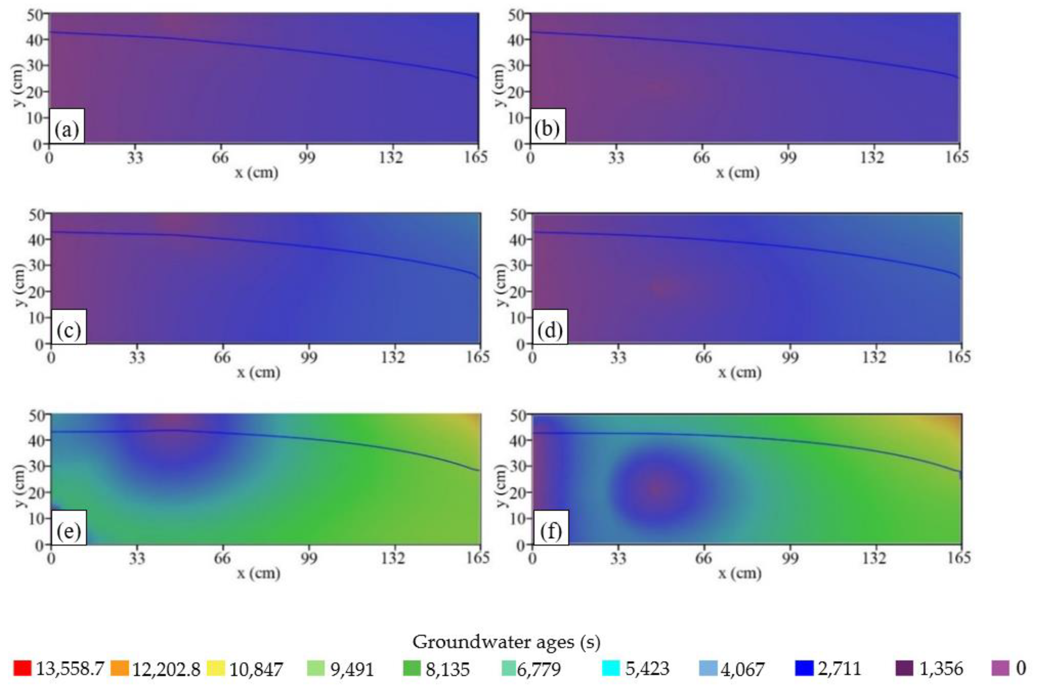
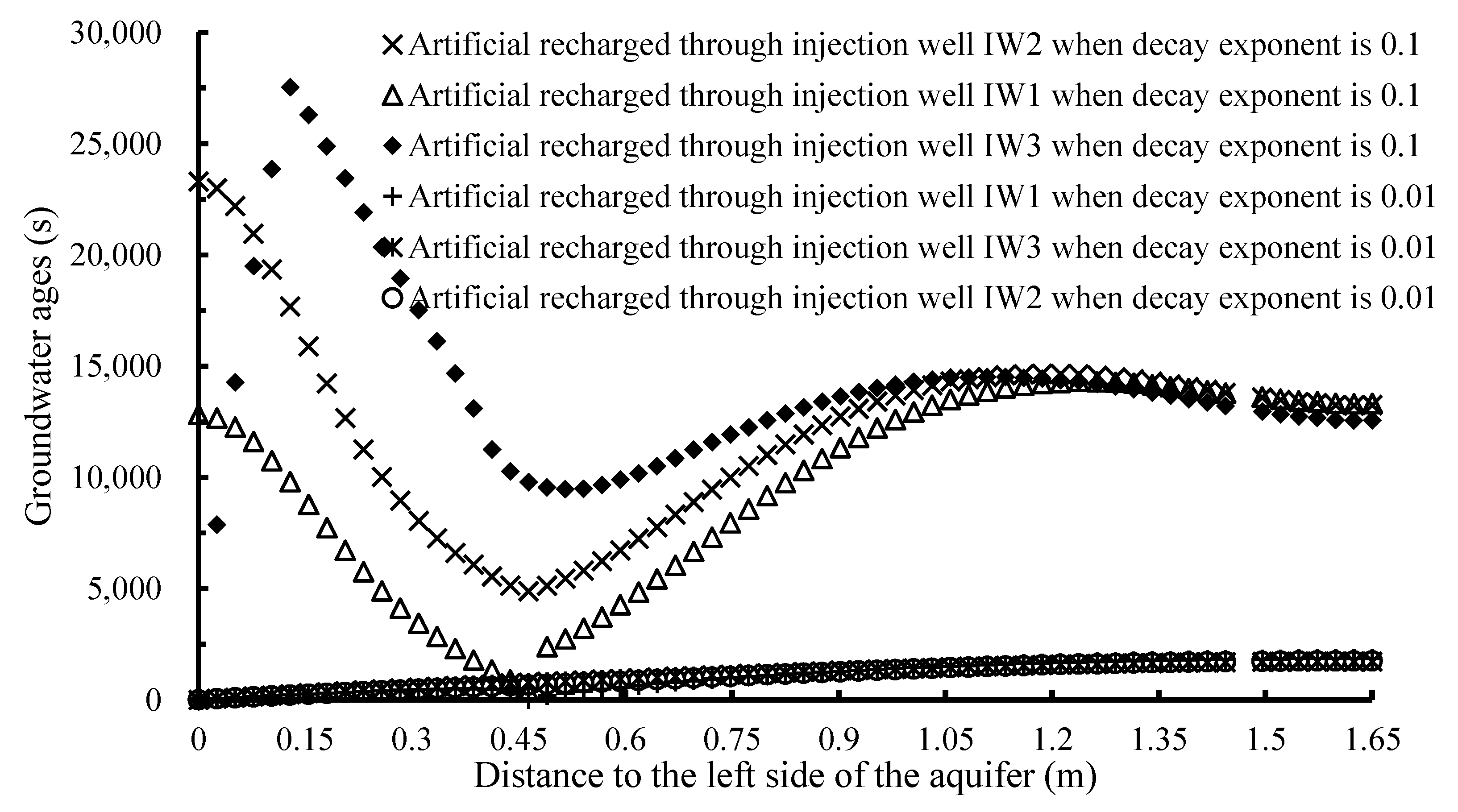
3.2. Groundwater Age

Figure 9 and Figure 10 show the groundwater age fields produced by the infiltration basin and injection well IW3 with variational decay exponents of K in different directions. It can be seen that the smaller artificial recharge rate (the artificial recharge rate in infiltration basin is 5 and 0.2 m/d in injection well IW3) has a limited effect on the groundwater age distribution when the decay exponents were small. The groundwater age always increased along the flow direction from upstream to downstream area with the decaying K. For example, groundwater age ranged from 0 to 2547.3 s (Figure 9a,b) when the depth-decay exponents were set to 0.01 m⁻¹. As shown in Figure 10a,b, age mainly ranged from 0 to 2711 s when the length-decay exponents were set to 0.005 m⁻¹. Furthermore, the increasing decay exponents can also increase the groundwater age and expand the degree of influence of the artificial recharge on groundwater age distribution. Taking left side figures in Figure 9 as an example, with the increase of depth-decay exponents, the spatial variability of groundwater age becomes increasingly obvious.

Figure 11 shows the groundwater age along the bottom of the aquifer induced by injection at different locations with variational depth-decay exponents, indicating little distinction for the age along the aquifer bottom when the decay exponent was small. On the contrary, the variation of groundwater age showed an obvious distinction when the decay exponent was larger. The results shown by Figure 11 could also demonstrate that the decaying K could expand the degree of influence of artificial recharge on the distributions of groundwater age.

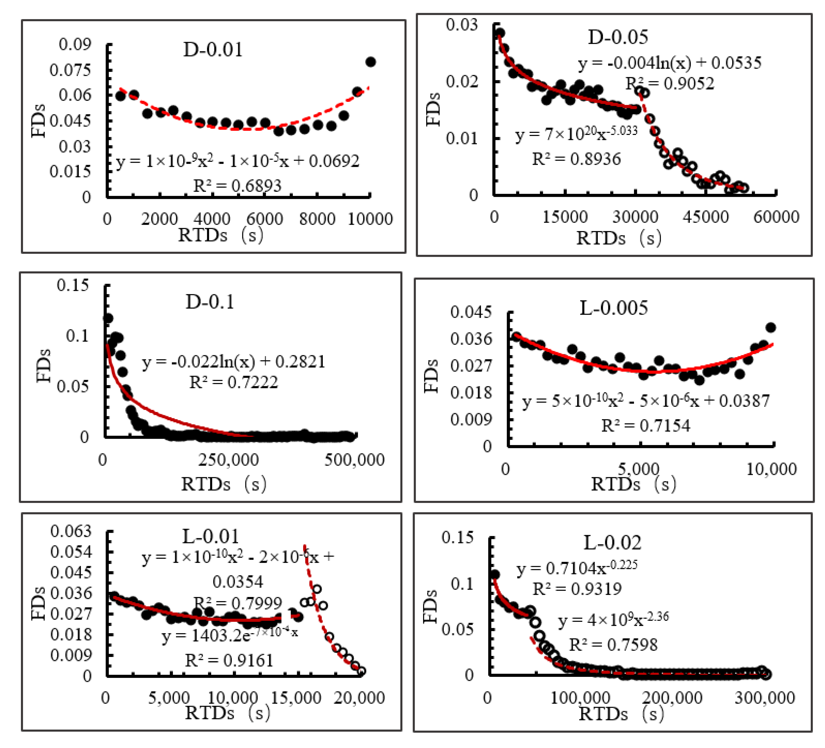
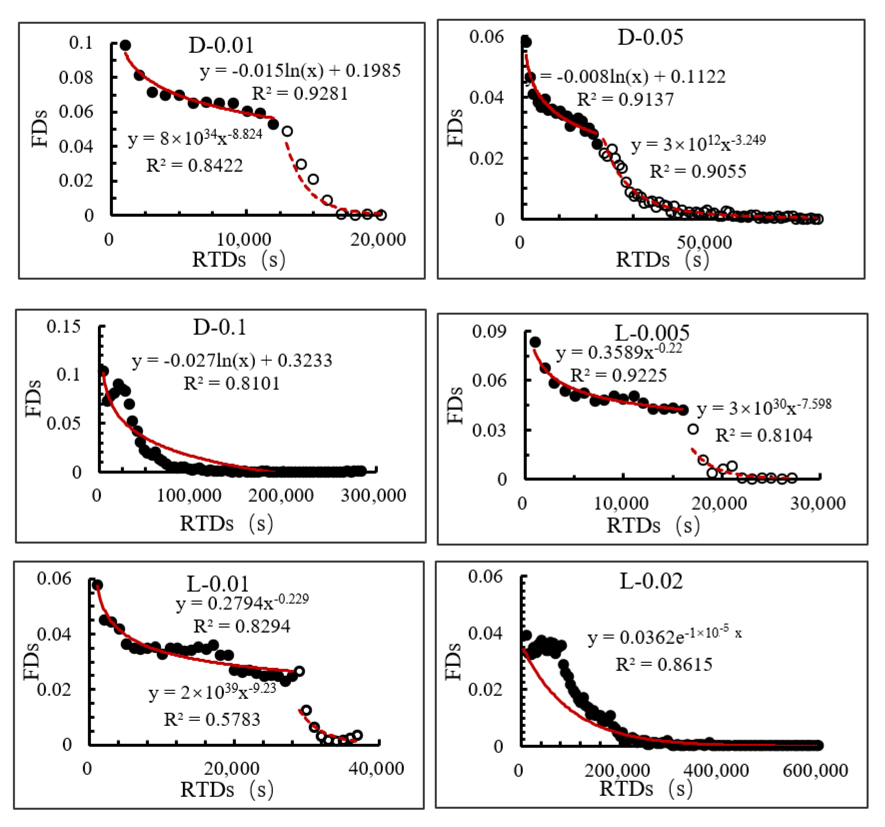
3.3. Residence Time Distributions

RTDs of the sand tank phreatic aquifer induced by artificial recharge and decaying hydraulic conductivity were considered. The results showed that not only the ambient groundwater but also the artificially recharged water exhibit different RTD laws with the decaying K in different directions and different decay exponents. Taking the RTDs driven by injection at well IW1 as an example, the frequency distributions (FDs) to RTDs of artificially recharged water driven by variational decay exponents are shown in Figure 12, and those of ambient groundwater are shown in Figure 13. The results of depth-decay condition (Figure 12), with a smaller decay exponent (when the depth-decay exponent was set to 0.01 m⁻¹), showed the fitted trend line for FDs to RTDs toward a quadratic polynomial law and the frequency of different residence time showed less distinction. With the increase of depth-decay exponents, when the depth-decay exponent was set to 0.05 m⁻¹, the fitted trend line for FDs to RTDs was divided into two steps: the early step toward a logarithmic behavior and the later step toward a power behavior. When the depth-decay exponent was set to a sufficiently large value (A₁ = 0.1 m⁻¹), the two-step fitted trend line merged into one and toward a logarithmic behavior. Furthermore, similar results could be obtained with the K decay in the length direction. With the increase of the length-decay exponents, the fitted lines for FDs to RTDs exhibited a quadratic polynomial behavior and then was divided into two steps. Decay of K in different directions could affect the RTD behavior obviously.

FDs to RTDs of ambient groundwater are shown in Figure 13, with different decay direction and decay exponents of K when artificially recharged at injection well IW1. In contrast to the RTD behaviors of artificially recharged water, when the decay exponents were set to smaller values, the fitted trend lines for FDs to RTDs always showed two steps. However, the two-step lines were merged into one when the decay exponents were set to larger values. Most of the artificially recharged water RTD fitted trend lines showed logarithmic behavior and power behavior.

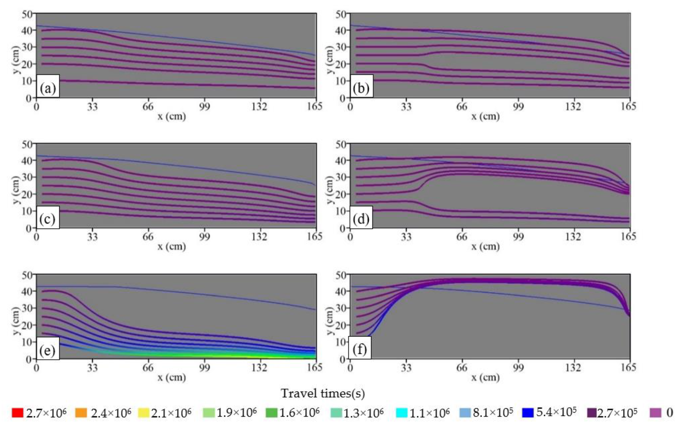
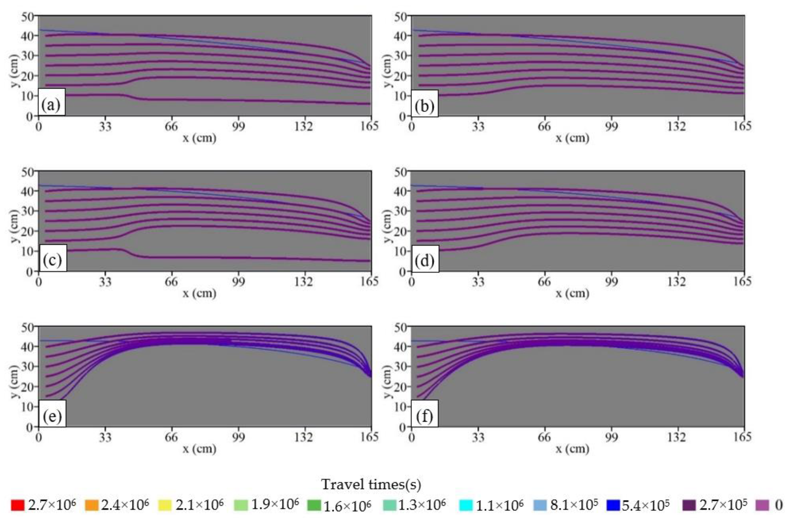
3.4. Ambient Groundwater Flow Paths

Ambient groundwater flow paths induced by artificial recharge and decaying K were considered here. Several particles were released at tracing points in the numerical model on the left side to trace the ambient groundwater flow. Taking those produced by the infiltration basin and injection well IW3 in the aquifer with decaying K as examples, the ambient groundwater flow paths are shown in Figure 14 and Figure 15 with different decay directions. The left panel of Figure 14 shows the flow paths driven by the infiltration basin and variational decay exponents in the depth direction, indicating that the increasing decay exponents could increase the penetration depth and travel times of ambient groundwater. The penetration depth here means the depth of certain groundwater flow paths at certain sections. The right panel of Figure 14 shows the ambient groundwater flow paths induced by injection well IW3 and decaying K in the depth direction. With the increase of depth-decay exponents, the ambient groundwater flow paths were gradually fractionated by artificial recharge, meaning that the penetration depth of shallow layer’s flow decreased with the increasing decay exponent, in contrast to that of the deep layer. The penetration depth of the ambient groundwater flow paths was decreased by the decaying K when the decay exponent was sufficiently large. Similar to the results shown by right panel of Figure 14, the ambient groundwater flow paths could also be found gradually fractionated by the screen of injection wells with the increase of the length-decay exponents when artificially recharged through injection well IW2. In contrast to those shown by Figure 14 and the left panel of Figure 15, the right panel of Figure 15 shows that the penetration depth of ambient groundwater flow paths decreased with the increase of the length-decay exponents when artificially recharged by injection well IW1. Furthermore, with the change of ambient groundwater flow paths, travel times could also be increased by the increasing decay exponents.

3.5. Artificially Recharged Water Lens

An artificially recharged water lens was formed in artificial recharge areas due to artificially induced recharge to the lens. The interface between artificially recharged water and ambient groundwater is a part of the boundary of such lenses. Artificially recharged water lenses produced by the infiltration basin and injection wells in the aquifer with decaying K are shown in Figure 16 and Figure 17, in the form of a tracing-line cluster from infiltration basins or injection wells. Left panels of Figure 16 and Figure 17 show the artificially recharged water lenses produced by the infiltration basins with different decay directions and decay exponents, indicating that the increasing decay exponents increased the thickness of the artificially recharged water lens and the travel times of artificially recharged water. The penetration depth of the interface of artificially recharged–ambient groundwater gradually increased with the increase of decay exponents and moved to the deep layers of the aquifer. Especially when the length-decay exponent was set to a sufficiently large value (A₂ = 0.002 m⁻¹, Figure 17e), the aquifer was almost filled with artificially recharged water, and the left recharge boundary became a discharge boundary. The right panels of Figure 16 show that the thickness of the artificially recharged water lens increased with the increasing depth-decay exponent, with the up-interface moving to the shallow layer and the down-interface to deep layer. Similar results can also be seen in right panel of Figure 17 when the decay of K was set in the length direction and artificially recharged through injection well IW1. With the increase of length-decay exponents, the interface of the artificially recharged–ambient groundwater interface gradually moved to the shallow layer, and the thickness of the artificially recharged water lens increased. Furthermore, with the increase of decay exponents, increased travel times could be seen in every scenario.

4. Discussion

Alluvial plains are always deeply affected by human activities and richness of fresh groundwater [47]. Artificial recharge involves intensive activities to regulate water resources and represents a major factor in controlling the groundwater flow system on a regional scale [15]. At the same time, the spatial variation law of K in aquifers is fundamental to understanding the groundwater flow processes. Thus, based on the depositional features of the alluvial fan, lab-scale experiments and numerical simulations were performed in this study to investigate the groundwater flow features under the combined effects of artificial recharge and decaying K. Settings of artificial recharge modes were adopted from Wu et al. [15] and generalized from the Tailan river basin. Because surface water flowing through alluvial fans in arid and semiarid areas is often disconnected from groundwater, the infiltration basin was set to a prescribed flux (Neumann type) boundary [15,41,48].

The gradual decline in K with depth and length is a hallmark of piedmont alluvial fan hydrogeology [17,19], which influences features of subsurface flow such as the distribution of path lines, velocity, and residence time along these path lines. Depth-dependent K is a manifestation of regional-scale heterogeneity and was widely observed in the geological medium [20,35,36,37,49]. Different relationships of K with depth have been fitted in different sites with different K range, for example, the power function [23], logistic function [23], and exponential function [33]. In our analysis, the aquifer was isotropic, and an exponentially decaying function was used to describe the decrease of K with depth for the similar K range to that of Ameli et al. [20]. There is a lack of data and results on the variation law of K with length from apex to apron area in alluvial fans, but the variation trend could be generalized based on the depositional features of Tailan alluvial fans. Thus, considering that the main purpose of this study was to investigate the groundwater flow induced by artificial recharge and the decaying K, here we assumed an exponentially decaying function to describe the gradual decrease of K with length from apex to apron area in the alluvial fan.

Previous research on groundwater flow under depth decay conditions was performed by Jiang et al. [35] and Ameli et al. [20]. Jiang’s [35] results showed that the development of local versus regional flow systems is sensitive to the depth-decay exponent of K. With higher rates of decrease in K with depth, the penetration depth of local flow systems increases. That is, penetration depth of flow path from a certain recharge point decreased with the increase of depth-decay exponents. Similar to Jiang’s [35] results, Ameli et al. [20] demonstrated that the increasing depth-decay exponents decreased the penetration depth of flow paths. In contrast with the previous work, numerical simulations conducted in this study showed that the penetration depth of flow paths from infiltration basin increased with the increase of depth-decay exponents. The opposite results were attributed to the differences of boundary conditions. In Jiang’s [35] and Ameli’s [20] studies, no flux boundaries were set to the left and right boundary in the numerical model, but they were constant head boundaries in this study. The main flow directions of ambient groundwater were horizontal when the constant head boundary was used in the model. With the increase of decay exponents, the horizontal flow velocities were lower and exerted less influence on the artificially recharged water flow, which was almost vertical. Thus, the resultant velocities were almost vertical, and the penetration depth was deeper.

The RTDs, the descriptions of residence times from recharge to discharge areas, determine the type and rate of many biological, biochemical, and geochemical processes occurring on the surface, near the surface, and in deep environments [34]. The most commonly used model used for RTDs is the exponential model [50], and some recent studies demonstrated that regional and multiscale flow systems exhibit a power law [34,50,51]. RTDs driven by human activities, such as artificial recharge and exploitation, exhibit different laws with the natural state. Most of them showed exponential law and logarithmic behavior [15]. According to Cardenas and Jiang’s [34] results, the RTDs for both a simple basin with one flow system and a basin with nested local and regional systems gradually evolve to a power law RTD with exponentially depth-decreasing K and porosity. Here, the results from the numerical simulations demonstrated that the combined effect of artificial recharge and decaying K could lead to a different RTD behavior compared with the previous studies. That is, some of the sub-steps exhibit logarithmic law behavior or quadratic polynomial law behavior.

Notably, similar to the results presented by Wu et al. [15], the groundwater flow could pass across the water table, which is common in the simulated results and lab-scale experiments. This was attributed to the limitation of using the small-scale model. In the lab-scale model, the capillary zone thickness relative to the saturated zone thickness was extremely large in these simulations, which seems unreasonable when considering a field-scale case. The capillary zone, in agreement with Lehmann et al. [52], was 13 and 25 cm for packed sand in this study. Thus, the limitation did not affect the main purpose of this study (i.e., understanding how decaying hydraulic conductivity and artificial recharge affect the groundwater flow dynamics). As such, the process of groundwater flow in these experiments and simulations was plausible.

The differences in properties between ambient groundwater and artificially recharged water were not taken into account in this study, although, to the best of our knowledge, the artificial recharge accelerated the interaction of surface water and groundwater. Especially when artificially recharged through the injection wells, the physical and chemical properties of artificially recharged water are different from those of ambient groundwater due to the absence of vadose filtration of the aquifer and the corresponding physical and chemical reactions. For example, the temperature difference between surface and groundwater has been widely observed in many sites worldwide and used to trace the water flow [44,53,54]. Artificial recharge also increases the overall dissolved oxygen (DO) concentration in recharged areas, as it is commonly believed that DO concentration of groundwater is much lower than that of surface water [55]. Thus, accurate simulation of the artificially recharged water lenses and the artificially recharged–ambient groundwater interface was essential to developing adequate groundwater management and protection schemes. According to the results of this paper, decaying K increases the thickness of the artificially recharged water lens and changes the locations of the artificially recharged–ambient groundwater interface compared with the homogeneous conditions.

Due to economic development, population growth, urbanization, and irrigation-area increase, human activities are being viewed as the main driver of hydrogeological processes [49,56,57]. However, when coupled with the decaying K, which has been widely observed in geological medium both in the depth direction and length direction in alluvial fan areas, the groundwater flow processes caused by human activities increase. As shown by the results of this study, ambient groundwater and artificially recharged water flow paths, groundwater age distributions, locations of stagnation points, RTDs, and the locations of the artificially recharged–ambient groundwater interface were totally different from each other with the variation of decay direction and exponents. Thus, the decay of K should not be neglected when analyzing hydrological problems related to artificial regulated groundwater flow. In other words, based on the results of this study, neglecting the decaying K may cause an underestimation of the effect of human activities on groundwater systems.

5. Conclusions

Human activities and medium characteristics represent the major factors in controlling the groundwater flow system on a regional scale. Zonal heterogeneity and layered heterogeneity of K were applied in numerical models to investigate groundwater flow affected by human activities. The systematic decrease in K in a certain direction, especially with length, was seldom accounted for in studies on groundwater flow. Based on the lab-scale sand tank and depositional features of the alluvial fan, lab experiments and numerical simulations were performed in this study to investigate the variation of groundwater flow under the combined influences of artificial recharge and decaying K with the depth and length direction. The lab-scale sand tank experiments and numerical simulations demonstrated that the groundwater flow features induced by artificial recharge were significantly controlled by the decaying K. The decay of K with depth or length in alluvial fan areas expanded the degree of influence of artificial recharge on ambient groundwater flow processes.

Our findings also have some practical implications for the performance of managed aquifer recharge. Based on these results, recommendations for the performance of MAR in alluvial fan aquifers could be made as follows: (a) A relatively low artificial recharge rate should be adopted in alluvial fan aquifers, so as not to affect the natural groundwater cycle significantly. (b) The screening of recovery wells should be much longer than that for homogeneous aquifers in order to capture more recharged water, as the thickness of the artificially recharged water lens is much larger in an alluvial fan aquifer with decaying hydraulic conductivity. (c) More attention should be paid to the water quality, as the chemical loading rates were strongly controlled by the groundwater flow paths, which change much more obviously in an alluvial fan aquifer. (d) A relatively low pumping rate should be adopted in managed alluvial fan aquifers, as the increased groundwater age due to decaying hydraulic conductivity results in a low cycle rate.

References

1. Cao, G.; Scanlon, B.R.; Han, D.; Zheng, C. Impacts of thickening unsaturated zone on groundwater recharge in the North China Plain. J. Hydrol. 2016, 537, 260–270. [Google Scholar] [CrossRef]
2. Hsu, N.-S.; Chiang, C.-J.; Wang, C.-H.; Liu, C.-W.; Huang, C.-L.; Liu, H.-J. Estimation of pumpage and recharge in alluvial fan topography under multiple irrigation practices. J. Hydrol. 2013, 479, 35–50. [Google Scholar] [CrossRef]
3. Kendy, E.; Gérard-Marchant, P.; Walter, M.T.; Zhang, Y.; Liu, C.; Steenhuis, T.S. A soil-water-balance approach to quantify groundwater recharge from irrigated cropland in the North China Plain. Hydrol. Process. 2003, 17, 2011–2031. [Google Scholar] [CrossRef]
4. Tan, X.-C.; Wu, J.-W.; Cai, S.-Y.; Yang, J.-Z. Characteristics of Groundwater Recharge on the North China Plain. Ground Water 2013, 52, 798–807. [Google Scholar] [CrossRef]
5. Wang, B.; Jin, M.; Nimmo, J.R.; Yang, L.; Wang, W. Estimating groundwater recharge in Hebei Plain, China under varying land use practices using tritium and bromide tracers. J. Hydrol. 2008, 356, 209–222. [Google Scholar] [CrossRef]
6. Liu, Y.; Yamanaka, T.; Zhou, X.; Tian, F.; Ma, W. Combined use of tracer approach and numerical simulation to estimate groundwater recharge in an alluvial aquifer system: A case study of Nasunogahara area, central Japan. J. Hydrol. 2014, 519, 833–847. [Google Scholar] [CrossRef]
7. Foster, S.; Garduno, H.; Evans, R.; Olson, D.; Tian, Y.; Zhang, W.; Han, Z. Quaternary Aquifer of the North China Plain?assessing and achieving groundwater resource sustainability. Hydrogeol. J. 2004, 12, 81–93. [Google Scholar] [CrossRef]
8. Eastoe, C.J.; Hutchison, W.R.; Hibbs, B.J.; Hawley, J.; Hogan, J.F. Interaction of a river with an alluvial basin aquifer: Stable isotopes, salinity and water budgets. J. Hydrol. 2010, 395, 67–78. [Google Scholar] [CrossRef]
9. Galloway, D.L.; Burbey, T.J. Review: Regional land subsidence accompanying groundwater extraction. Hydrogeol. J. 2011, 19, 1459–1486. [Google Scholar] [CrossRef]
10. Liu, Y.; Yamanaka, T. Tracing groundwater recharge sources in a mountain–plain transitional area using stable isotopes and hydrochemistry. J. Hydrol. 2012, 464–465, 116–126. [Google Scholar] [CrossRef] [Green Version]
11. Famiglietti, J.S.; Lo, M.; Ho, S.L.; Bethune, J.; Anderson, K.J.; Syed, T.H.; Swenson, S.C.; de Linage, C.R.; Rodell, M. Satellites measure recent rates of groundwater depletion in california’s central valley. Geophys. Res. Lett. 2011, 38. [Google Scholar] [CrossRef] [Green Version]
12. Choi, B.-Y.; Yun, S.-T.; Mayer, B.; Chae, G.-T.; Kim, K.-H.; Kim, K.; Koh, Y.-K. Identification of groundwater recharge sources and processes in a heterogeneous alluvial aquifer: Results from multi-level monitoring of hydrochemistry and environmental isotopes in a riverside agricultural area in Korea. Hydrol. Process. 2009, 24, 317–330. [Google Scholar] [CrossRef]
13. Du, X.Q.; Wang, Z.J.; Ye, X.Y. Potential clogging and fissolution effects during artificial recharge of groundwater using potable water. Water Resour. Manag. 2013, 27, 3573–3583. [Google Scholar] [CrossRef]
14. Du, X.; Ye, X.; Zhang, X. Clogging of saturated porous media by silt-sized suspended solids under varying physical conditions during managed aquifer recharge. Hydrol. Process. 2018, 32, 2254–2262. [Google Scholar] [CrossRef]
15. Wu, P.; Shu, L.; Yang, C.; Xu, Y.; Zhang, Y. Simulation of groundwater flow paths under managed abstraction and recharge in an analogous sand-tank phreatic aquifer. Hydrogeol. J. 2019, 27, 3025–3042. [Google Scholar] [CrossRef]
16. Saito, K.; Oguchi, T. Slop of alluvial fans in humid regions of Japan, Taiwan and the Philippines. Geomorphology 2005, 70, 147–162. [Google Scholar] [CrossRef]
17. Blair, T.C. Cause of dominance by sheet flood vs. debris flow processes on two adjoining alluvial fans, Death Valley, California. Sedimentology 1999, 46, 1015–1028. [Google Scholar] [CrossRef]
18. Chen, X.; Song, J.; Wang, W. Spatial variability of specific yield and vertical hydraulic conductivity in a highly permeable alluvial aquifer. J. Hydrol. 2010, 388, 379–388. [Google Scholar] [CrossRef]
19. Staley, D.M.; Wasklewicz, T.A.; Blaszczynski, J.S. Surficial patterns of debris flow deposition on alluvial fans in Death Valley, CA using airborne laser swath mapping data. Geomorphology 2006, 74, 152–163. [Google Scholar] [CrossRef]
20. Ameli, A.A.; Mcdonnell, J.; Bishop, K. The exponential decline in saturated hydraulic conductivity with depth: A novel method for exploring its effect on water flow paths and transit time distribution. Hydrol. Process. 2016, 30, 2438–2450. [Google Scholar] [CrossRef]
21. Price, W.G.; Potter, A.; Thomson, T.K.; Smith, G.E.P.; Hazen, A.; Beardsley, R.C. Discussion on dams on sand foundations. Trans. Am. Soc. Civ. Eng. 1911, 73, 190–208. [Google Scholar] [CrossRef]
22. Jia, Y.F.; Guo, H.M.; Jiang, Y.X.; Wu, Y.; Zhou, Y.Z. Hydrogeochemical zonation and its implication for arsenic mobi-lization in deep groundwaters near alluvial fans in the Hetao Basin, Inner Mongolia. J. Hydrol. 2014, 518, 410–420. [Google Scholar] [CrossRef]
23. Chen, Y.-F.; Ling, X.-M.; Liu, M.-M.; Hu, R.; Yang, Z. Statistical distribution of hydraulic conductivity of rocks in deep-incised valleys, Southwest China. J. Hydrol. 2018, 566, 216–226. [Google Scholar] [CrossRef]
24. Achtziger-Zupancic, P.; Loew, S.; Hiller, A. Factors controlling the permeability distribution in fault vein zones sur-rounding granitic intrusions (Ore Mountains/Germany). J. Geophys. Res. Solid Earth 2017, 122, 1876–1899. [Google Scholar]
25. Cheng, C.; Song, J.; Chen, X.; Wang, D. Statistical distribution of streambed vertical hydraulic conductivity along the Platte River, Nebraska. Water Resour. Manag. 2010, 25, 265–285. [Google Scholar] [CrossRef] [Green Version]
26. Hess, K.M.; Wolf, S.H.; Celia, M.A. Large-scale natural gradient tracer test in sand and gravel, Cape Cod, Massachusetts: 3. Hydraulic conductivity variability and calculated macrodispersivities. Water Resour. Res. 1992, 28, 2011–2027. [Google Scholar] [CrossRef]
27. Rehfeldt, K.R.; Boggs, J.M.; Gelhar, L.W. Field study of dispersion in a heterogeneous aquifer: 3. Geostatistical analysis of hydraulic conductivity. Water Resour. Res. 1992, 28, 3309–3324. [Google Scholar] [CrossRef]
28. Lu, C.; Qin, W.; Zhao, G.; Zhang, Y.; Wang, W. Better-fitted probability of hydraulic conductivity for a silty clay site and its effects on solute transport. Water 2017, 9, 466. [Google Scholar] [CrossRef] [Green Version]
29. Faulkner, D.; Armitage, P. The effect of tectonic environment on permeability development around faults and in the brittle crust. Earth Planet. Sci. Lett. 2013, 375, 71–77. [Google Scholar] [CrossRef]
30. Stober, I.; Bucher, K. Hydraulic conductivity of fractured upper crust: Insights from hydraulic tests in boreholes and fluid-rock interaction in crystalline basement rocks. Geofluids 2014, 15, 161–178. [Google Scholar] [CrossRef]
31. Morrow, C.A.; Lockner, D.A. Permeability differences between surface-derived and deep drillhole core samples. Geophys. Res. Lett. 1994, 21, 2151–2154. [Google Scholar] [CrossRef] [Green Version]
32. Ku, C.-Y.; Hsu, S.-M.; Chiou, L.-B.; Lin, G.-F. An empirical model for estimating hydraulic conductivity of highly disturbed clastic sedimentary rocks in Taiwan. Eng. Geol. 2009, 109, 213–223. [Google Scholar] [CrossRef]
33. Saar, M.O.; Manga, M. Depth dependence of permeability in the Oregon Cascades inferred from hydrogeologic, thermal, seismic, and magmatic modeling constraints. J. Geophys. Res. Space Phys. 2004, 109. [Google Scholar] [CrossRef] [Green Version]
34. Cardenas, M.B.; Jiang, X.W. Groundwater flow, transport, and residence times through topography-driven basins with exponentially decreasing permeability and porosity. Water Resour. Res. 2010, 46, W11538. [Google Scholar] [CrossRef] [Green Version]
35. Jiang, X.-W.; Wan, L.; Wang, X.-S.; Ge, S.; Liu, J. Effect of exponential decay in hydraulic conductivity with depth on regional groundwater flow. Geophys. Res. Lett. 2009, 36, 36. [Google Scholar] [CrossRef]
36. Jiang, X.-W.; Wang, X.-S.; Wan, L.; Ge, S. An analytical study on stagnation points in nested flow systems in basins with depth-decaying hydraulic conductivity. Water Resour. Res. 2011, 47, 47. [Google Scholar] [CrossRef] [Green Version]
37. Rumynin, V.; Leskova, P.; Sindalovskiy, L.; Nikulenkov, A. Effect of depth-dependent hydraulic conductivity and anisotropy on transit time distributions. J. Hydrol. 2019, 579, 124161. [Google Scholar] [CrossRef]
38. Nakaya, S.; Uesugi, K.; Motodate, Y.; Ohmiya, I.; Komiya, H.; Masuda, H.; Kusakabe, M. Spatial separation of groundwater flow paths from a multi-flow system by a simple mixing model using stable isotopes of oxygen and hydrogen as natural tracers. Water Resour. Res. 2007, 43. [Google Scholar] [CrossRef]
39. Polizzotto, M.L.; Kocar, B.D.; Benner, S.G.; Sampson, M.; Fendorf, S. Near-surface wetland sediments as a source of arsenic release to ground water in Asia. Nat. Cell Biol. 2008, 454, 505–508. [Google Scholar] [CrossRef] [PubMed]
40. Qin, D.J.; Zhao, Z.F.; Han, L.F. Determination of groundwater recharge regime and flow path in the Lower Heihe River basin in an arid area of Northwest China by using environmental tracers: Implications for vegetation degradation in the Ejina Oasis. Appl. Geochem. 2012, 27, 1133–1145. [Google Scholar] [CrossRef]
41. Wang, W.; Li, J.; Feng, X.; Chen, X.; Yao, K. Evolution of stream-aquifer hydrologic connectedness during pumping—Experiment. J. Hydrol. 2011, 402, 401–414. [Google Scholar] [CrossRef]
42. Keeler, B.L.; Gourevitch, J.D.; Polasky, S.; Isbell, F.; Tessum, C.W.; Hill, J.D.; Marshall, J.D. The social costs of nitrogen. Sci. Adv. 2016, 2, e1600219. [Google Scholar] [CrossRef] [PubMed] [Green Version]
43. Mi, L.; Xiao, H.; Zhang, J.; Yin, Z.; Shen, Y. Evolution of the groundwater system under the impacts of human activities in middle reaches of Heihe River Basin (Northwest China) from 1985 to 2013. Hydrogeol. J. 2016, 24, 971–986. [Google Scholar] [CrossRef]
44. Xie, Y.; Batlle-Aguilar, J. Limits of heat as a tracer to quantify transient lateral river-aquifer exchanges. Water Resour. Res. 2017, 53, 7740–7755. [Google Scholar] [CrossRef]
45. Atlabachew, A.; Shu, L.; Wu, P.; Zhang, Y.; Xu, Y. Numerical modeling of solute transport in a sand tank physical model under varying hydraulic gradient and hydrological stresses. Hydrogeol. J. 2018, 26, 2089–2113. [Google Scholar] [CrossRef]
46. Xin, P.; Yuan, L.R.; Li, L.; Barry, D.A. Tidally driven multi-scale pore water flow in a creek-marsh system. Water Resour. Res. 2011, 47, 209–216. [Google Scholar] [CrossRef]
47. Filippini, M.; Stumpp, C.; Nijenhuis, I.; Richnow, H.; Gargini, A. Evaluation of aquifer recharge and vulnerability in an alluvial lowland using environmental tracers. J. Hydrol. 2015, 529, 1657–1668. [Google Scholar] [CrossRef]
48. Wang, W.K.; Li, J.T.; Wang, W.M.; Chen, X.H.; Cheng, D.H.; Jia, J. Estimating streambed parameters for a disconnected river. Hydrol. Process. 2014, 28, 3627–3641. [Google Scholar] [CrossRef]
49. Wang, W.; Zhu, Y.; Dong, S.; Becker, S.; Chen, Y. Attribution of decreasing annual and autumn inflows to the Three Gorges Reservoir, Yangtze River: Climate variability, water consumption or upstream reservoir operation? J. Hydrol. 2019, 579, 124180. [Google Scholar] [CrossRef]
50. Cardenas, M.B. Potential contribution of topography-driven regional groundwater flow to fractal stream chemistry: Residence time distribution analysis of Tóth flow. Geophys. Res. Lett. 2007, 34, 05403. [Google Scholar] [CrossRef]
51. Kollet, S.J.; Maxwell, R.M. Demonstrating fractal scaling of baseflow residence time distributions using a fully-coupled groundwater and land surface model. Geophys. Res. Lett. 2008, 35, 07402. [Google Scholar] [CrossRef]
52. Lehmann, P.; Stauffer, F.; Hinz, C.; Dury, O.; Flühler, H. Effect of hysteresis on water flow in a sand column with a fluc-tuating capillary fringe. J. Contam. Hydrol. 1998, 33, 81–100. [Google Scholar] [CrossRef]
53. Sawyer, A.H.; Cardenas, M.B.; Bomar, A.; Mackey, M. Impact of dam operations on hyporheic exchange in the riparian zone of a regulated river. Hydrol. Process. 2009, 23, 2129–2137. [Google Scholar] [CrossRef]
54. Lu, C.; Chen, S.; Jiang, Y.; Shi, J.; Yao, C.; Su, X. Quantitative analysis of riverbank groundwater flow for the Qinhuai River, China, and its influence factors. Hydrol. Process. 2018, 32, 2734–2747. [Google Scholar] [CrossRef]
55. Lu, S.; Wagner, R.; Schmidt, M.; Wiseman, L. Impact of Groundwater Seepage Flow on DO TMDL Development. Proc. Water Environ. Fed. 2009, 2009, 3246–3262. [Google Scholar] [CrossRef]
56. Yang, T.; Zhang, Q.; Wang, W.; Yu, Z.; Chen, Y.D.; Lu, G.; Hao, Z.; Báron, A.; Zhao, C.; Chen, X.; et al. Review of advances in hydrologic science in china in the last decades: Impact study of climate change and human activities. J. Hydrol. Eng. 2013, 18, 1380–1384. [Google Scholar] [CrossRef]
57. Jakóbczyk-Karpierz, S.; Sitek, S.; Jakobsen, R.; Kowalczyk, A. Geochemical and isotopic study to determine sources and processes affecting nitrate and sulphate in groundwater influenced by intensive human activity—carbonate aquifer Gliwice (southern Poland). Appl. Geochem. 2017, 76, 168–181. [Google Scholar] [CrossRef]
Figure 1. (a) Schematic diagram of the sand tank and the experimental apparatus; (b) side view of the laboratory-scale numerical model setup with prescribed boundary conditions. The boundaries on the right and left sides were set to a constant head boundary condition. The 19 red points in (a) are the pressure transducers for the hydraulic head data acquisition. The three black points in (a) are the injection wells. The red line in (b) on the top boundary was set to a flux boundary condition. The three red points in (b) are injection wells.
Water 13 01649 g001
Figure 2. Variation of hydraulic conductivity along the distance from apex to apron zone in the Tailan river basin.
Water 13 01649 g002
Figure 3. Hydraulic conductivity fields with different depth-decay exponents. (a) the decay exponent was set to 0.01 m−1, (b) the decay exponent was set to 0.05 m−1, (c) the decay exponent was set to 0.1 m−1.
Water 13 01649 g003
Figure 4. The exponential relationship between hydraulic conductivity and depth.
Water 13 01649 g004
Figure 5. Hydraulic conductivity fields with different length-decay exponents. (a) the decay exponent was set to 0.005 m−1, (b) the decay exponent was set to 0.01 m−1, (c) the decay exponent was set to 0.02 m−1.
Water 13 01649 g005
Figure 6. The exponential relationship between hydraulic conductivity and length.
Water 13 01649 g006
Figure 7. Flow fields when artificially recharged through the infiltration basin (left side figures) and injection well IW3 (right side figures) with different depth-decay exponents. The depth-decay exponents in (a) and (b) were set to 0.01 m−1. The depth-decay exponents in (c) and (d) were set to 0.05 m−1. The depth-decay exponents in (e) and (f) were set to 0.1 m−1. The blue lines in the figures represent the water table.
Water 13 01649 g007
Figure 8. Flow fields when artificially recharged through the infiltration basin (left side figures) and injection well IW3 (right side figures) with different length-decay exponents. The length-decay exponents in (a) and (b) were set to 0.005 m−1. The length-decay exponents in (c) and (d) were set to 0.01 m−1. The length-decay exponents in (e) and (f) were set to 0.02 m−1. The blue lines in the figures represent the water table.
Water 13 01649 g008
Figure 9. Groundwater age driven by depth-decaying hydraulic conductivity and artificial recharge through the infiltration basin (left side) and injection well IW3 (right side). The depth-decay exponents in (a) and (b) were set to 0.01 m−1. The depth-decay exponents in (c) and (d) were set to 0.05 m−1. The depth-decay exponents in (e) and (f) were set to 0.1 m−1. The blue lines in the figures represent the water table.
Water 13 01649 g009
Figure 10. Groundwater age driven by artificial recharge through the infiltration basin (left side figures) and injection well IW3 (right side figures) with different length-decay exponents. The length-decay exponents in (a) and (b) were set to 0.005 m−1. The length-decay exponents in (c) and (d) were set to 0.01 m−1. The length-decay exponents in (e) and (f) were set to 0.02 m−1. The blue lines in the figures represent the water table.
Water 13 01649 g010
Figure 11. Groundwater age at the bottom of the aquifer driven by artificial recharge through injection wells at different locations and different decay exponents.
Water 13 01649 g011
Figure 12. Frequency distribution of RTDs of artificially recharged water (injection well IW1) with different decay direction and decay exponents of hydraulic conductivity. “D-0.01” means the depth-decay exponent was set to 0.01, and “L-0.005” means the length-decay exponent was set to 0.005. The red lines are fitted trend lines.
Water 13 01649 g012
Figure 13. Frequency distribution of RTDs of ambient groundwater with different decay direction and decay exponents of hydraulic conductivity. “D-0.01” means the depth-decay exponent was set to 0.01, and “L-0.005” means the length-decay exponent was set to 0.005. The red lines are fitted trend lines.
Water 13 01649 g013
Figure 14. Ambient groundwater flow paths associated with travel time produced by artificial recharge and different depth-decay exponents. The left panel of figures were produced by the infiltration basin and the right panel of figures were produced by injection well IW3. The depth-decay exponents in (a) and (b) were set to 0.01 m−1. The depth-decay exponents in (c) and (d) were set to 0.05 m−1. The depth-decay exponents in (e) and (f) were set to 0.1 m−1. The blue lines in the figures represent the water table.
Water 13 01649 g014
Figure 15. Ambient groundwater flow paths associated with travel time produced by artificial recharge and different length-decay exponents. The left panel of figures were produced by injection well IW2 and the right panel of figures were produced by injection well IW1. The length-decay exponents in (a) and (b) were set to 0.005 m−1. The length-decay exponents in (c) and (d) were set to 0.01 m−1. The length-decay exponents in (e) and (f) were set to 0.02 m−1. The blue lines in the figures represent the water table.
Water 13 01649 g015
Figure 16. Artificially recharged water lens associated with travel times (TTs) produced by the infiltration basin (left panel of the figures) and injection well IW3 (right panel of the figures) with different depth-decay exponents. The depth-decay exponents in (a) and (b) were set to 0.01 m−1. The depth-decay exponents in (c) and (d) were set to 0.05 m−1. The depth-decay exponents in (e) and (f) were set to 0.1 m−1. The blue lines in the figures represent the water table. The yellow points in the figures are the locations of injection wells. The red lines are flow paths of artificially recharged water. The rainbow lines are flow paths of artificially recharged water.
Water 13 01649 g016
Figure 17. Artificially recharged water lens associated with travel times (TTs) produced by the infiltration basin (left panel of the figures) and injection well IW1 (right panel of the figures) with different length-decay exponents. The length-decay exponents in (a) and (b) were set to 0.005 m−1. The length-decay exponents in (c) and (d) were set to 0.01 m−1. The length-decay exponents in (e) and (f) were set to 0.02 m−1. The blue lines in the figures represent the water table. The yellow points in the figures are the locations of injection wells. The rainbow lines are flow paths of artificially recharged water.
Water 13 01649 g017
Publisher’s Note: MDPI stays neutral with regard to jurisdictional claims in published maps and institutional affiliations.