Performance Analysis for Road-Bioretention with Three Types of Curb Inlet Using Numerical Model

Abstract

The FullSWOF-ZG (Full Shallow Water Overland Flow with infiltration determined by Zones and Grate-inlet submodules) program was used to simulate the road-bioretention (RB) stripe and evaluate the performance of the RB stripe with three types of curb inlet. The program was revised from the open-source FullSWOF-2D program and the validation results indicated FullSWOF-ZG predicts the RB stripe performance accurately. The model cases of 27 RB with different longitude slopes (S₀), cross slopes (S_x), and curb inlet lengths (L_ci) for the undepressed, composite depressed, and local depressed curb inlets were established in this study. Therefore, 81 cases in total were simulated to explore the curb inlet type and design parameter’s influence on the RB stripe performance. Overall, it was found that the bioretention control efficiency will increase with the S₀ decrease, S_x increase, and L_ci increase. The composite depressed curb inlet was the most efficient to intercept the road runoff into the bioretention strip, the next best is the local depressed curb inlet, and the undepressed curb inlet was the least efficient. The curb inlet and grate inlet combination in composite depressed curb inlet cases were able to deal with all the road surface runoff for the small longitudinal slope (S₀ = 0.1% and 0.3%) to relieve the road local flood inundation.

1. Introduction

To endorse sustainable urbanization plans, the Sponge City (SPC) paradigm based on green/gray stormwater management infrastructure integration was announced in 2013 as a relief countermeasure to urban syndromes such as water shortage, water pollution, flood inundation, and ecologic deterioration in China [1,2]. As an important component of SPC, road-bioretention (RB) [3,4] is a water quantity and quality control practice that benefits decreasing surface runoff, increasing groundwater recharge, and treating various pollutants through a variety of processes [5,6]. The bioretention facilities near a road could be individual isolated cells and long stripes or plots along a road (Figure 1), which receive the runoff from the road surface and/or other adjacent surfaces. Figure 1a shows the plan view for a road-bioretention stripe that includes the road surface with longitudinal (S₀) and cross (S_x) slopes, a curb inlet, a grate inlet along the roadside, the bioretention stripe, an overflow great inlet and a berm near the end of the bioretention stripe, and the curb separating the road and bioretention. Typically, the RB stripe has the same or a similar longitudinal slope of the road. It may have several RB stripes separated by berms, especially when the longitudinal slope is large. The curb inlet length is L_ci (see the description for all symbols listed in Abbreviation part). The RB stripe that combine green/gray infrastructures to facilitate road runoff control through infiltration and ponding as well as relieve road local flood inundation risk is widely used in pilot SPC construction in China [7].

Traditional curb inlets are to intercept the surface runoff into the underground stormwater pipeline network, but the curb inlets for the RB stripes are to intercept the surface runoff into the bioretention facilities to store, retain, infiltrate the runoff to remove the pollutants and improve the water quality. Two types of curb inlets are commonly used over the world: the undepressed and composite depressed curb inlets. Figure 1b and Figure 2a show the undepressed curb inlet with a single cross slope S_x at any cross-sections, e.g., along the road and passing the curb inlet, which is section A–A in Figure 1. The composite depressed curb inlet is shown in Figure 1c and Figure 2b placed along gutters of the street, and has a composite section with two cross slopes (S_x for the road and S_w for the gutter over a width of w_com) at all sections along the road. The third type of curb inlet is the local depressed curb inlet shown in Figure 1d and Figure 2c which has a local depression over the opening length of the inlet but a single cross slope S_x for all other parts of the road. The local depressed inlet is widely used in some SPC pilot projects in China [7] for improving the inlet interception efficiency. In various construction projects, the local depressed inlet could be constructed using a composite slope S_w over the gutter width w_com (Figure 1d) or just simply cuts the road to form a small depression (Figure 2c) over the curb inlet length. The local depressed curb inlet is also different from Texas type C and D curb inlets [8,9] that have 1.52 m (5 ft) transition before and after the local depression over the inlet opening. The transition before the inlet is to change the cross slope gradually from S_x to S_w (S_w > S_x) in the gutter width or from S_w to S_x after the inlet. Type C and D inlet could be more efficient for intercepting the surface runoff but it is more complex to construct in the field or should be precast.

Most of the previous studies point out that bioretention has good hydrologic performance and pollutant removal efficiency dealing with urban road runoff based on experimental and monitored data [10]. There was barely any detailed guidance and study on the influence of longitudinal slope and cross slope of the road as well as the opening length and the type (Figure 1 and Figure 2) of curb inlet on RB stripe performance that could be found in China [11,12]. Li et al. [13] emphasized the importance of inlet hydraulics and the spatial distribution of inflow for a road-bioretention stripe, and they proposed and integrated a hydraulic and hydrologic modeling approach to simulate the overall runoff control performance of the RB stripe. Li et al. [14] conducted a full-scale laboratory RB stripe numerical experiments and simulation to explore the influence of S₀ and S_x on RB stripe performance while the experiment scenarios were limited to explore the detailed influence of different parameters.

It is a complex problem to design the RB stripe that needs to consider the curb inlet interception efficiency, grate inlet capacity, as well as the bioretention ponding and infiltration capacity systematically to make the RB stripe perform well on road runoff control. The influence of design parameters on the RB stripe with undepressed curb inlet (Figure 1b) was studied in a previous study [15] while the RB stripe performance with different types of curb inlet (Figure 1) still needs to be explored. Understanding and clarifying the influence of design parameters (S₀, S_x, and L_ci) and curb inlet type on RB stripe performance is particularly important and useful to SPC construction in China [16]. In this study, the FullSWOF-ZG (Full Shallow Water Overland Flow with infiltration determined by Zones and Grate-inlet submodules) program [17], that has a submodule determining the different rainfall, infiltration, and friction in zones, as well as the two-dimensional–one-dimensional (2D–1D) surface-to-grate-inlet flow exchange submodule, was used to explore the RB stripe performance and design concerns. The program was revised from the open-source hydraulic program FullSWOF-2D (version 1.07, Lab. J. A. Dieudonné and EPU Nice Sophia, Nice, France) [17] that solves the full shallow-water equations (SWEs) for overland flow (OF) in 2D simulation domain. With the help of the validated FullSWOF-ZG program, the objective of this study is to explore the mechanism and influence of those design parameters on RB stripe performance through building numerical models for different scenarios.

2. Materials and Methods

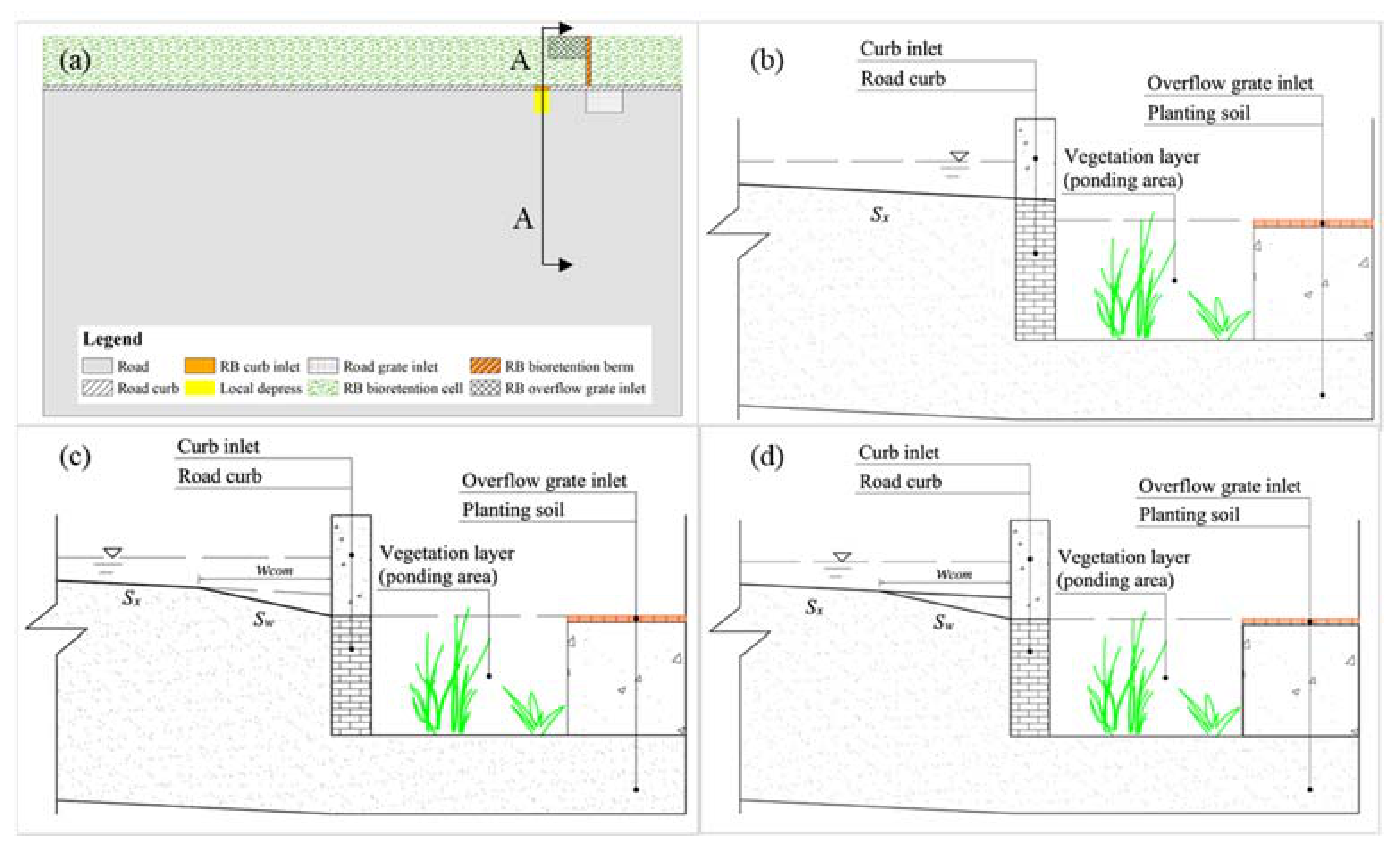
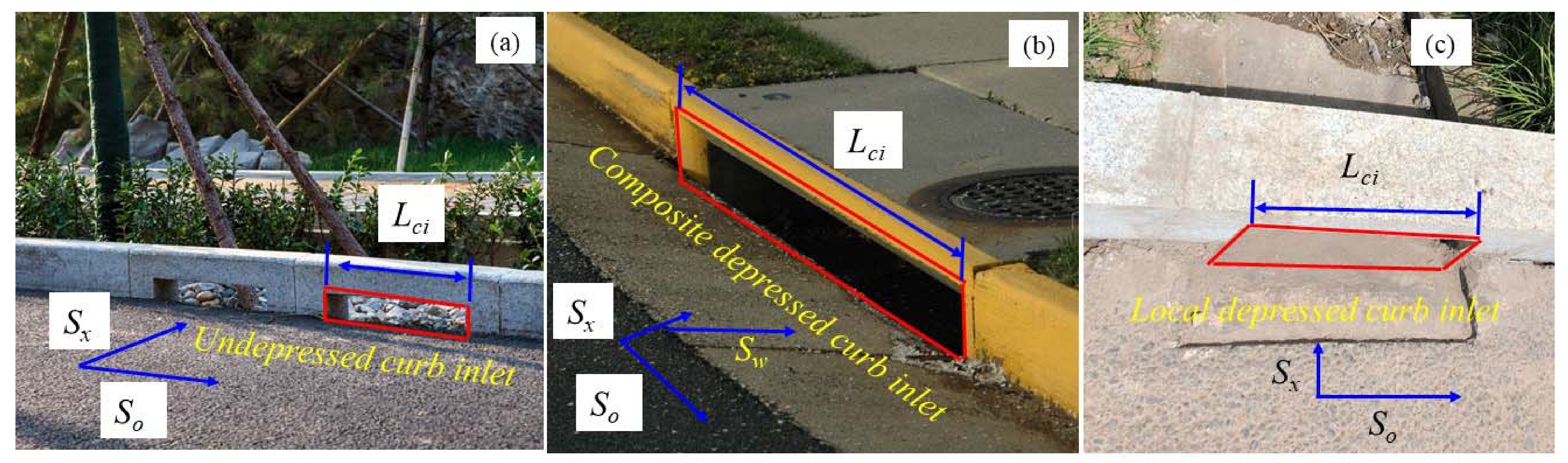
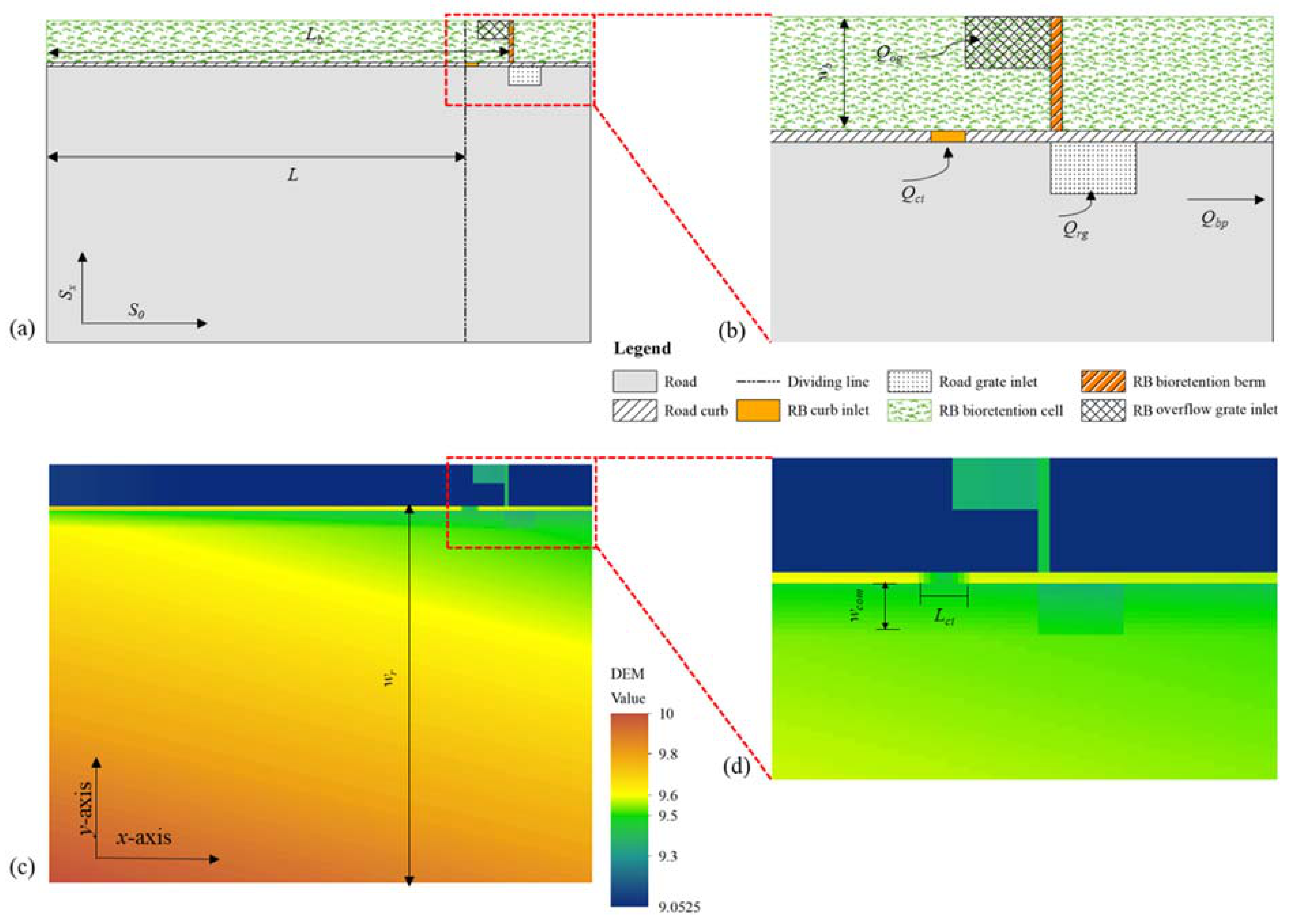
2.1. Road-Bioretention (RB) Stripe Design

Curb inlet interception efficiency, road grate inlet capacity, as well as the bioretention ponding and infiltration capacity, should be taken into consideration to design the RB stripe for better RB performance. Three types of curb inlet are commonly used in the USA and China (Figure 1 and Figure 2). The undepressed curb inlet with a single cross slope is widely used in China. The composite depressed curb inlet is commonly used in the USA [18]. The local depressed curb inlet used in some SPC pilot projects in China [19] is also studied here. Current curb inlet design practices in the USA are based on documents produced by the Federal Highway Administration entitled Hydraulic Engineering Circular No. 22 (HEC-22) [20] and Urban Street Stormwater Guide produced by the National Association of City Transportation Officials [11]. The design of commonly used inlet types is presented in HEC-22 and specific design guidance for other inlets is also provided in two previous studies [9,21].

The ponding depth of the RB stripe is controlled by the height of the overflow grate inlet and the berm height (Figure 1). The overflow height provides for the temporary storage of the stormwater before it filters downward through the bioretention facility. The temporary ponding depth for bioretention facilities range from 5 cm (for mitigating sidewalk runoff alone, or in fast-draining soils) to up to 30 cm (for mitigating roadway runoff, or in slower-draining soils) [11]. The Delaware Green Technologies Design Manual and Model provide design guidance for bioretention systems and allow a maximum ponding depth of 45 cm [22]. Davis et al. [6] declared the overall principles of bioretention ponding volume and infiltration capacity design in their study. The ponding volume is designed by the corresponding catchment area (e.g., contributing road surface are) and design rainfall depth. It also should be calculated based on the RB geometry such as bioretention length L_b, width w_b, and slope.

The bioretention design specifications envisioned the use of natural soils with high permeability [23]. Three soil textural classifications were specified which include: loamy sand, sandy loam, and loam. Sites with subsoils of an infiltration rate less than 13 mm/h are required to use an underdrain system that provides positive drainage to a defined outfall point [6]. The Green-Ampt model [17] was adapted to simulate the bioretention infiltration process in this study. The infiltration parameters include saturated hydraulic conductivity (K), moisture deficit (Δθ), and dry suction head (φ). In this study, RB stripe with loamy sand soil was modeled. The infiltration parameter values: K = 51 mm/h, Δθ = 0.410, φ = 0.09 m, were adapted based on the soil type [24]. The thickness of the soil layer is 0.45 m according to the bioretention design guidelines [25].

2.2. FullSWOF-ZG Program

As a Saint-Venant system [26], the simplified SWEs model is widely used to simulate the incompressible Navier–Stokes flow occurring in rivers, channels, ocean, and land surfaces [27]. The conservative form of the 2D SWEs for FullSWOF-2D program, including the continuity equation and two momentum equations for x- and y- directions, is stated as the following equations for each computational cell (center coordinates x and y):

$$\frac{\partial h}{\partial t}+\frac{\partial \left(hu\right)}{\partial x}+\frac{\partial \left(hv\right)}{\partial y}=R\left(x,y\right)-I\left(x,y\right)$$

(1)

$$\frac{\partial \left(hu\right)}{\partial t}+\frac{\partial }{\partial x}\left(h{u}^2+\frac{g{h}^2}{2}\right)+\frac{\partial }{\partial y}\left(huv\right)=gh\left(\frac{\partial z}{\partial x}-S_{fx}\right)$$

(2)

$$\frac{\partial \left(hv\right)}{\partial t}+\frac{\partial }{\partial x}\left(huv\right)+\frac{\partial }{\partial y}\left(h{v}^2+\frac{g{h}^2}{2}\right)=gh\left(\frac{\partial z}{\partial y}-S_{fy}\right)$$

(3)

where R (x, y) (m/s) is the cell’s rainfall intensity; I (x, y) (m/s) is the cell’s infiltration rate; h (m) is the cell’s water depth; z (m) is the cell topography elevation as a function of the cell location or x and y coordinates; u (m/s) and v (m/s) is the cell’s depth-averaged velocities in x and y directions, respectively; S_fx and S_fy are the cell’s friction slopes in x and y directions, respectively; g (m/s²) is gravity acceleration; t (s) is time.

The FullSWOF-2D program fully solves SWEs on a structured mesh (square cells) in two dimensions using the finite volume method (FVM) that ensures mass conservation [28]. A well-balanced numerical scheme was adapted to guarantee the positivity of water depth and the preservation of steady states for specific hydrological features such as during wet–dry transitions and tiny water depths [17,29]. Different boundary conditions, friction laws, and numerical schemes were developed that make the program a very powerful overland flow simulation software. A modified bi-layer (crust- and soil-layer) Green–Ampt (GA) infiltration model [30] to calculate I (x, y) for Equation (1) was coded in the FullSWOF-2D [28] that enables the program to simulate overland flow on impervious and pervious surfaces simultaneously.

The FullSWOF-2D program was revised and improved in this study: the updated FullSWOF-ZG program included the spatialized rainfall, infiltration, and friction determination as well as a new 2D-1D drainage inlet submodule. Therefore, the program can simulate impervious and pervious surfaces in the same domain simultaneously. The simulation domain can have several grate inlets, therefore, the 2D overland flow can drain into these 2D drainage inlets (rectangles) to become 1D flow in underground drainage pipes. Currently, the FullSWOF-ZG program does not further simulate 1D flow in the drainage pipes assuming the pipe capability is large enough to accept all inflow from inlets. The simulation domain has curb inlets connecting the road and bioretention where normally the runoff on the road flows through the curb inlet into the bioretention. The grate-inlet discharge capacity from the 2D overland flow to the 1D drainage pipe flow is calculated using the weir equation [31] applied to the cells surrounding the grate inlet.

The FullSWOF-ZG program was tested against the data from undepressed curb inlet cases in Spaliviero’s [32] study, local depressed curb inlet cases conducted by Hammonds and Holley [9], and overland flow on pervious surface cases measured and simulated by Esteves et al. [30], but this comprehensive model validation was presented elsewhere by Li et al. [14,15]. The differences of simulated and observed curb inlet interception efficiencies (∆E) ranged from −3.7% to 4.4% with an average $\pm$ standard deviation of 0.8 $\pm$ 2.6% for undepressed curb inlet cases [33]. The ∆E ranged from −3.2% to 13.2%, with an average $\pm$ standard deviation of 3.5 $\pm$ 3.5% for local depressed curb inlet cases [34]. In a previous study by Fang et al. [8], the ∆E ranged from −7.0% to 17.6%, with an average $\pm$ standard deviation of 1.0 $\pm$ 4.87% in their FLOW-3D simulations for local depressed curb inlet. The goodness of fit for the simulated hydrograph is evaluated using the Nash–Sutcliffe efficiency (NSE) coefficient [35]. The NSE coefficient of FullSWOF-ZG and Esteves’s study ranged from 0.64 to 0.95 (average $\pm$ standard deviation as 0.75 $\pm$ 0.11) and from 0.46 to 0.93 (0.79 $\pm$ 0.15) for overland flow on pervious surfaces simulation, respectively [36]. The simulated results for undepressed curb inlet, local depressed curb inlet, and overland flow on pervious surface cases were matched well with the observed data, which proves that the FullSWOD-ZG program can not only simulate overland flow on pervious and impervious surfaces accurately but can also predict the curb inlet efficiency very precisely.

2.3. Performance Evaluation Cases

Figure 3a shows the plan view for the road-bioretention modeling case which includes different parts of the RB stripe: the road with longitude and cross slopes, the bioretention, curb inlet, grate inlet on the road, a berm at the end of bioretention, and the curb separating the road and bioretention. The RB performance is affected by longitude slope S₀, cross slope S_x, curb inlet interception efficiency E_ci, bioretention depth D_b, overflow height h_b, and the RB’s soil infiltration parameters in

Table 1. Design parameters for RB stripes.

Parameters	L (m)	S0 [-]	Sx [-]	Lci (m)	Db (m)	K (mm/h)	φ (m)	Δθ [-]	Vpc (m3)
Value range	10	0.001–0.007	0.01–0.04	0.45–0.90	0.35	51	0.090	0.410	2.82–3.33

Note: L [m] is the road surface length in the upstream of the curb inlet, S₀ [-] is the longitudinal slope of the road-bioretention stripe, S_x [-] is the cross slope of the road, L_ci (m) is the curb inlet length, D_b (m) is the bioretention depth, K (mm/h) is the saturated hydraulic conductivity, φ (m) is the dry suction head, Δθ [-] is the moisture deficit, and V_pc (m³) is the calculated bioretention ponding volume.

. Different modeling cases were established to explore the influence of design parameters on RB performance. Even bioretention is flat in the y-direction with lower elevation (i.e., D_b) than the road surface, bioretention has the same length and longitude slope in the x-direction as the road does (Figure 3). Figure 3c,d show the full and zoomed-in view digital elevation models (DEMs) for the modeling cases with composite depressed Case 01 in

Table 2. Parameters of modeling cases for RB stripes with three types of curb inlet.

Case No.	S0 [-]	Sx [-]	Lci (m)
Case01	0.001	0.010	0.45
Case02	0.001	0.010	0.600
Case03	0.001	0.010	0.900
Case04	0.001	0.020	0.45
Case05	0.001	0.020	0.600
Case06	0.001	0.020	0.900
Case07	0.001	0.040	0.45
Case08	0.001	0.040	0.600
Case09	0.001	0.040	0.900
Case10	0.003	0.010	0.45
Case11	0.003	0.010	0.600
Case12	0.003	0.010	0.900
Case13	0.003	0.020	0.45
Case14	0.003	0.020	0.600
Case15	0.003	0.020	0.900
Case16	0.003	0.040	0.45
Case17	0.003	0.040	0.600
Case18	0.003	0.040	0.900
Case19	0.007	0.010	0.45
Case20	0.007	0.010	0.600
Case21	0.007	0.010	0.900
Case22	0.007	0.020	0.45
Case23	0.007	0.020	0.600
Case24	0.007	0.020	0.900
Case25	0.007	0.040	0.45
Case26	0.007	0.040	0.600
Case27	0.007	0.040	0.900

Note: S₀ [-] is the longitudinal slope of the road-bioretention stripe, S_x [-] is the cross slope of the road, L_ci (m) is the curb inlet length in Figure 3d, S₀, S_x, and L_ci are the same for each undepressed, composite depressed, and local depressed curb inlet case.

.

There is a berm at the end of bioretention to pond the runoff inside bioretention that is allowed for infiltration downward and possible overflow into a grate inlet. The berm height used in this study is large enough to prevent the longitudinal outflow from bioretention. There is a grate inlet at the end of bioretention where the grate inlet opening is above the bioretention ground surface. The elevation difference between the grate inlet opening and the bioretention ground surface is called the overflow height, h_b which is 0.30 m in this study. Only when the water depth near the grate inlet is greater than h_b, the runoff in bioretention will flow (Q_og in Figure 3a) into the grate inlet then to the underground drainage pipe system. Part of the runoff generated on the road surface after rainfall begins was intercepted by curb inlet (Q_ci in Figure 3a), then the extra runoff was captured by the road grate inlet (Q_rg in Figure 3a), and finally, the rest part of the runoff was discharged to road end (Q_bp in Figure 3a). The free outfall boundary condition was used for the downstream (right boundary) of the simulation domain to avoid runoff flow back to the upstream.

The bioretention ponding volume (V_pc) calculated for each modeling case in this study did not consider the vegetation volume fraction of the bioretention facility. For all cases, the ponding length is larger than the upstream bioretention length time longitudinal slope ($L_b\times S_0<h_b$), therefore, the V_pc was calculated using the following Equation (4):

$$V_{pc}=\left(L_b\times h_b-\frac{L_b^2\times S_0}{2}\right)\times w_b-h_b\times A_{gr}$$

(4)

where V_pc (m³) is the calculated ponding volume based on bioretention geometry, w_b (m) is the bioretention width (1 m), L_b (m) is upstream bioretention length, S₀ is bioretention longitudinal slope, and h_b (m) bioretention overflow height, A_gr (m²) is overflow grate inlet area.

For all cases, the whole simulation domain length and width are 13 m (x-direction, Figure 3) and 7.7 m (y-direction, Figure 3), respectively. The road length L (Figure 3a) and width w_r (Figure 3c) before the dividing line in Figure 3 are 10 m and 6.7 m, respectively. The runoff generated before the curb inlet was calculated by L, w_r, and rainfall intensity. When y = 0, it is the centerline of the road, when y = 6.7 m, it is the curb [37]. The curb inlet is located after the curb lasts 10 m to allow the runoff generated on the road surface to get into the bioretention. The width of the bioretention cell is 1.0 m (w_b in Figure 3b), and the maximum ponding depth or the bioretention depth D_b is set as 0.05 m above the grate inlet overflow height h_b, i.e., D_b = 0.35 and h_b = 0.30 m for all cases. The curb inlet length (L_ci = 0.45 m for the undepressed case 01) and composite depressed part width w_com = 0.30 m for composite and local depressed case. The road grate inlet is a rectangle of 0.75 m (along the x-direction) by 0.45 m and was made to be 0.05 m lower than the surrounding road surface cells for the model simulation here. The grate inlet in RB has the same size as the road grate inlet with 0.30 m higher than surrounding bioretention cells.

Twenty-seven cases for every type of curb inlet were simulated in this study by having three longitudinal slopes, three cross slopes, and three curb inlet lengths (Table 2). The RB stripe has eight key design parameters which include upstream catchment length L, longitudinal slope S₀, cross slope S_x, curb inlet length L_ci, overflow height h_b, saturated hydraulic conductivity K, dry suction head φ, and soil moisture deficit Δθ. To fully understand the RB stripe performance and the influence from each parameter will require setting a large number of modeling cases, which is not studied here. Only the influence of RB stripe geometry, as well as the curb inlet type and length, were explored in this study which parameters for every case were shown in Table 2. Therefore, the loamy sand which was commonly used in the road-bioretention stripe was adopted in all simulation cases with the parameters K = 51 mm/h, Δθ = 0.41, and φ = 0.09 m.

The computational cell/grid size for the simulation domain is 0.05 m both in x- and y- directions with a total of 40,040 cells for all cases. There are total 135 cells in each grate inlet [(0.75/0.05) $\times$ (0.45/0.05)]. All cell’s elevations were calculated using a MATLAB program when the bottom left corner reference cell’s elevation (the highest in the domain) was assumed to be 10 m as shown in Figure 3c. The road surface and bioretention ground elevations, therefore, vary with longitudinal and cross slopes set for each modeling case (Table 2). All cells for the 0.1 m curb were set 0.2 m higher than the road surface cells. The cell’s elevations inside the curb inlet cells were calculated using the same cross slope of the road surface, which helps and allows the runoff to flow into the bioretention. The uniform rainfall intensity is 6.94 $\times$ 10⁻⁵ m/s (250 mm/h) and last 1200 s (20 min) to generate enough runoff to reach the ponding volume, but the total simulation period is 2400 s.

3. Results and Discussion

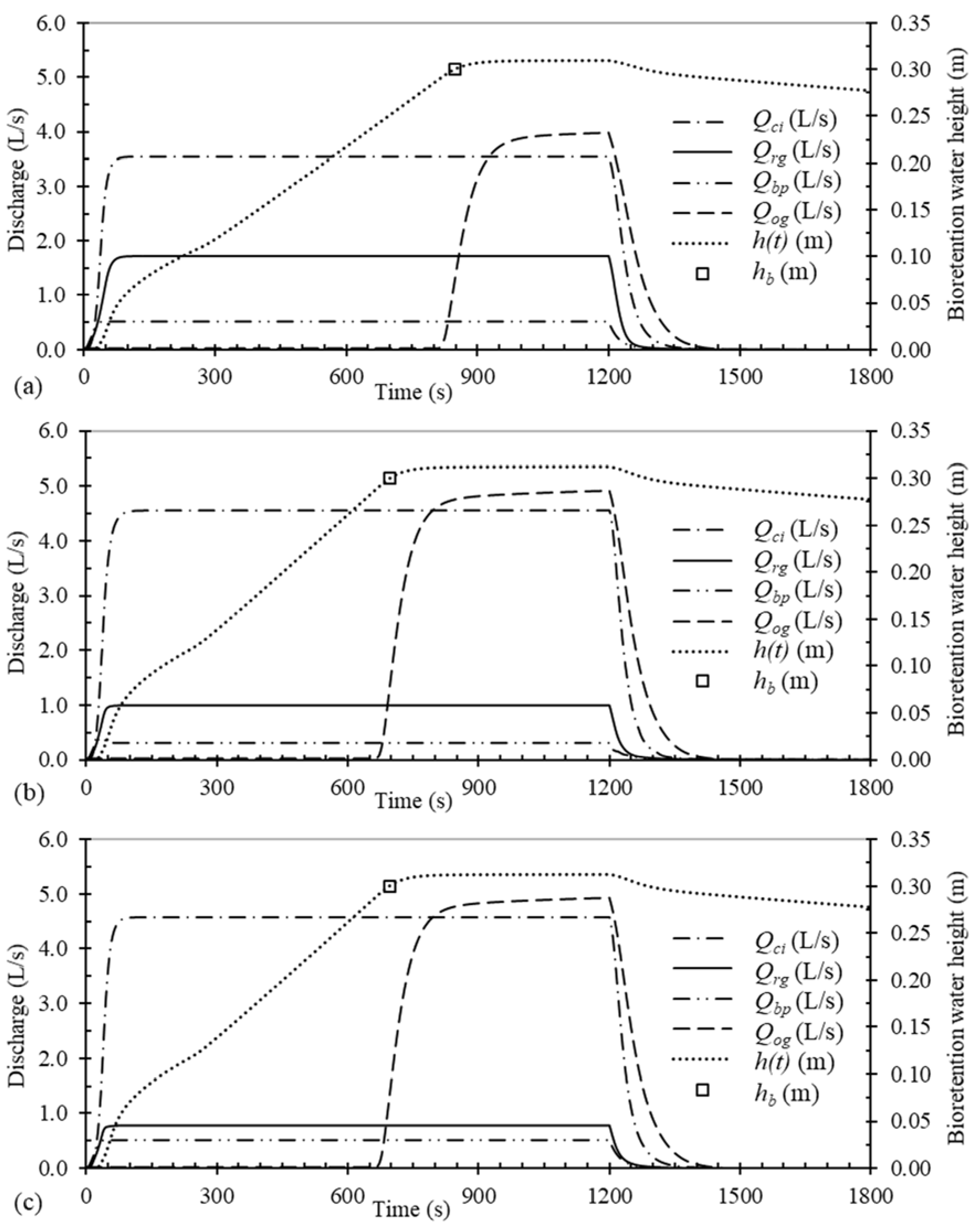
3.1. Simulated Hydrograph of RB Modeling Cases

As an example of modeling results for the RB stripe, the performances of the case Und27, Com27, and Loc27 were first evaluated and compared in Figure 4. Figure 4 shows the simulated hydrograph and bioretention water depth of three cases Und27, Com27, and Loc27. The upstream catchment length L = 10 m, longitudinal slope S₀ = 0.007, cross slope S_x = 0.04, curb inlet opening length L_ci = 0.90 m, overflow grate inlet height h_b = 0.30 m for cases Und27, Com27, and Loc27.

The hydrograph of curb inlet intercepted flow (Q_ci), road grate inlet captured flow (Q_rg), road end bypass flow (Q_bp), and the bioretention grate inlet overflow (Q_og) are shown in Figure 4. The rainfall intensity was 250 mm/h and maintained to 1200 s (20 min) for all simulation cases. Therefore, all hydrograph grow slowly at the beginning of the rainfall then reach the peak discharge and start to decrease after the rainfall stopped. The peak discharge of Q_ci was 3.544 L/s for Und27, 4.557 L/s for Com27, and 4.575 L/s for Loc27 which shows the composite and local depressed curb inlet have similar and larger interception capacity than the undepressed curb inlet. The peak discharge of Q_gr was 1.721 L/s for Und27, 0.996 L/s for Com27, and 0.782 L/s for Loc27 which shows that the composite gutter improved the grate inlet capture efficiency compared to the local depressed case. The peak discharge of Q_bp was 0.516 L/s for Und27, 0.416 L/s for Com27, and 0.516 L/s for Loc27 which shows the road-bioretention with composite curb inlet discharge the smallest runoff flow to the downstream road. The peak discharge (Q_pog) was 3.982 L/s for Und27, 4.918 L/s for Com27, and 4.930 L/s for Loc27, respectively. The Q_pog for Und27 was the smallest which due to the undepressed curb inlet intercepted the smallest runoff volume into the bioretention in this case. The overflow beginning time for Und27, Com27, and Loc27 was also 820 s, 673 s, and 673 s when the water depth in the bioretention becomes higher than the overflow grate inlet height. The detailed comparison results for all cases with three types of curb inlet is shown in

Table 3. Simulation discharge results of all road-bioretention cases.

Case No.	Qpci (L/s)			Qprg (L/s)			hmax (m)			Tbog (s)			Qpog (L/s)
	Und	Com	Loc	Und	Com	Loc	Und	Com	Loc	Und	Com	Loc	Und	Com	Loc
Case01	1.49	3.97	3.18	4.51	3.39	3.02	0.21	0.32	0.32	-	841	1023	-	4.29	3.44
Case02	1.91	4.54	3.50	4.16	2.65	2.72	0.25	0.32	0.32	-	759	956	-	4.87	3.81
Case03	2.65	4.97	4.06	3.44	1.90	2.15	0.31	0.32	0.32	1172	721	865	1.47	5.30	4.38
Case04	1.99	4.04	3.96	4.38	3.42	2.51	0.26	0.32	0.32	-	822	847	-	4.36	4.28
Case05	2.51	4.61	4.29	3.82	2.68	2.16	0.31	0.32	0.32	1203	743	803	0.77	4.94	4.61
Case06	3.43	5.03	4.78	2.80	1.95	1.58	0.32	0.32	0.32	958	706	750	3.87	5.37	5.11
Case07	2.52	4.10	4.61	4.09	3.41	2.11	0.31	0.32	0.32	1184	807	742	1.10	4.43	4.93
Case08	3.15	4.65	4.83	3.41	2.73	1.84	0.32	0.32	0.32	1003	734	722	3.54	4.99	5.15
Case09	4.23	5.05	5.07	2.21	1.98	1.44	0.32	0.32	0.32	812	700	708	4.63	5.39	5.41
Case10	1.24	3.67	2.86	3.55	2.41	2.28	0.19	0.32	0.31	-	859	1066	-	4.00	3.03
Case11	1.59	4.22	3.15	3.33	1.84	2.10	0.23	0.32	0.31	-	773	994	-	4.55	3.45
Case12	2.26	4.62	3.66	2.94	1.38	1.78	0.29	0.32	0.31	-	731	896	-	4.97	3.99
Case13	1.74	3.83	3.73	3.69	2.47	1.85	0.24	0.32	0.32	-	825	851	-	4.16	4.05
Case14	2.22	4.39	4.04	3.28	1.89	1.60	0.29	0.32	0.32	-	743	804	-	4.73	4.37
Case15	3.11	4.81	4.52	2.52	1.42	1.24	0.31	0.32	0.32	989	702	747	3.54	5.16	4.86
Case16	2.30	3.93	4.43	3.39	2.46	1.37	0.30	0.32	0.32	1242	806	733	0.20	4.26	4.76
Case17	2.91	4.47	4.64	2.82	1.90	1.21	0.31	0.32	0.32	1022	729	711	3.30	4.81	4.98
Case18	3.98	4.87	4.89	1.86	1.46	1.03	0.32	0.32	0.32	815	692	695	4.39	5.22	5.23
Case19	0.87	3.17	2.42	3.06	1.65	1.90	0.17	0.31	0.31	-	898	1124	-	3.50	2.06
Case20	1.15	3.64	2.66	2.90	1.23	1.77	0.20	0.31	0.31	-	807	1052	-	3.98	2.88
Case21	1.69	4.01	3.08	2.60	0.97	1.55	0.25	0.31	0.31	-	758	949	-	4.36	3.42
Case22	1.34	3.46	3.36	3.47	1.76	1.62	0.22	0.31	0.31	-	828	853	-	3.81	3.70
Case23	1.77	4.00	3.64	3.13	1.29	1.41	0.26	0.31	0.31	-	740	805	-	4.35	3.98
Case24	2.58	4.42	4.09	2.47	0.98	1.10	0.31	0.31	0.31	1051	693	744	2.93	4.78	4.44
Case25	1.93	3.61	4.13	3.12	1.76	1.03	0.28	0.31	0.31	-	797	714	-	3.96	4.47
Case26	2.51	4.14	4.33	2.60	1.30	0.90	0.31	0.31	0.31	1056	716	692	2.83	4.49	4.68
Case27	3.54	4.56	4.58	1.72	1.00	0.78	0.31	0.31	0.31	820	673	673	3.98	4.92	4.93

Note: Q_pci (L/s) is road curb inlet peak discharge for RB cases, Q_prg (L/s) is road grate inlet peak discharge, h_max (m) is the maximum bioretention water depth, T_bog (s) is the time of bioretention overflow start, Q_pog (L/s) is bioretention overflow peak discharge, “-“ means there is no overflow occurred in the bioretention.

.

As shown in Table 3, the average $\pm$ standard deviation of Q_pci is 2.32 $\pm$ 0.85 L/s for undepressed curb inlet cases, 4.25 $\pm$ 0.50 L/s for composite depressed curb inlet cases, and 3.94 $\pm$ 0.71 L/s for local depressed curb inlet cases, respectively. The simulation results show that the composite gutter will improve the curb inlet interception efficiency to a large extent. The peak curb inlet interception efficiency varies a lot for the undepressed curb inlet cases. The average $\pm$ standard deviation of Q_prg is 3.16 $\pm$ 0.69 L/s for undepressed curb inlet cases, 1.97 $\pm$ 0.72 L/s for composite depressed curb inlet cases, and 1.71 $\pm$ 0.55 L/s for local depressed curb inlet cases, respectively. The Q_prg for undepressed curb inlet cases was the largest which means the largest portion of runoff was discharged into the drainage pipe. The simulation results show the composite depressed gutter improves the grate inlet capture capacity when the Q_prg is compared to local depressed cases.

As shown in Table 3, bioretention overflow did not occur in 14 cases where the maximum water depth (h_max) did not reach the overflow height (h_b) during the whole simulation period. The bioretention overflow beginning time (T_bog) and overflow peak discharge (Q_pog) is mainly related to the curb inlet flow volume (V_ci) and bioretention overflow height (h_b). The average $\pm$ standard deviation of Q_pog is 2.81 $\pm$ 1.39 L/s for undepressed curb inlet cases, 4.59 $\pm$ 0.50 L/s for composite depressed curb inlet cases, and 4.24 $\pm$ 0.80 L/s for local depressed curb inlet cases. Case09 has the largest peak overflow discharge among these 27 cases. The overflow first occurs at 812 s then reached the highest overflow peak discharge as 4.63 L/s for undepressed case Und09. The overflow first occurs at 700 s and 708 s for Com09 and Loc09 then reached the highest overflow peak discharge as 5.39 L/s and 5.41 L/s, respectively. The bioretention overflow time (T_bog) was delayed when the curb inlet inflow volume (V_ci) decreases and overflow water height (h_b) increase.

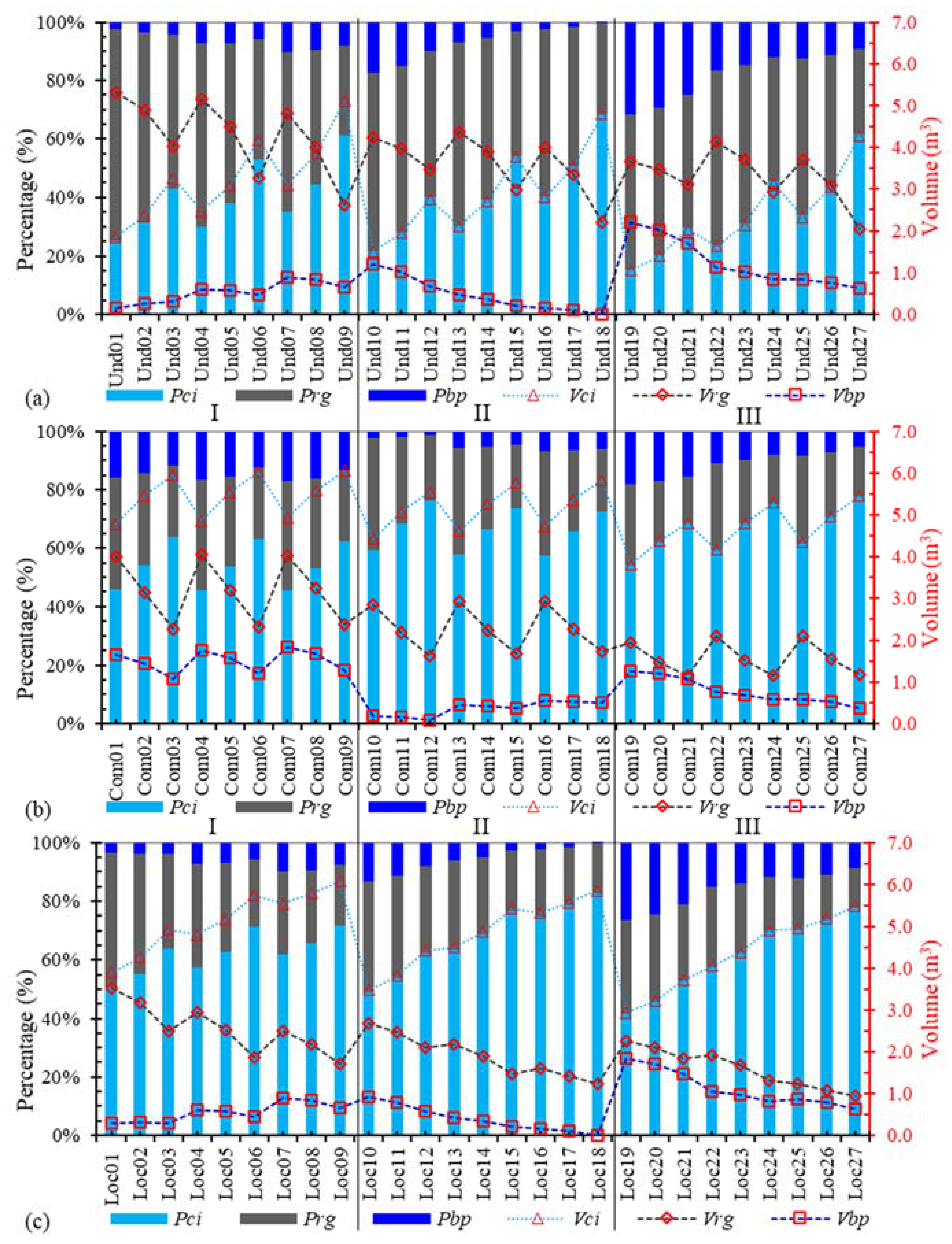
3.2. Intercepted and Captured Volume Analysis

Figure 5 shows different part runoff volumes and percentages for road-bioretention cases with three types of curb inlets. In Figure 5, group I are results for cases with S₀ = 0.001, group II are results for cases with S₀ = 0.003, and group III are results for cases with S₀ = 0.007. Figure 5a and

Table 4. Simulation results of road-bioretention cases with three types of curb inlet.

Name	Vci (m3)			Vrg (m3)			Vbp (m3)			Vbog (m3)			Vinf (m3)			Vbio (m3)			(Vinf + Vbio)/Vrb			∆V (%)
	Und	Com	Loc	Und	Com	Loc	Und	Com	Loc	Und	Com	Loc	Und	Com	Loc	Und	Com	Loc	Und	Com	Loc	Und	Com	Loc
Case01	1.86	4.78	3.89	5.32	4.00	3.52	−0.16	−1.65	−0.28	0.03	1.69	0.79	1.19	1.35	1.33	1.86	2.84	2.86	0.36	0.50	0.50	−1.32	−1.29	−1.31
Case02	2.36	5.46	4.27	4.89	3.14	3.17	−0.26	−1.46	−0.30	0.03	2.31	1.12	1.25	1.37	1.35	2.33	2.88	2.91	0.43	0.51	0.51	−1.25	−1.22	−1.24
Case03	3.25	5.95	4.93	4.02	2.26	2.50	−0.32	−1.08	−0.28	0.24	2.71	1.67	1.34	1.40	1.38	2.97	2.96	2.99	0.52	0.52	0.52	−1.10	−1.07	−1.09
Case04	2.46	4.86	4.80	5.16	4.04	2.93	−0.60	−1.77	−0.60	0.03	1.77	1.69	1.25	1.35	1.35	2.40	2.84	2.86	0.44	0.50	0.50	−1.28	−1.27	−1.28
Case05	3.08	5.54	5.18	4.49	3.18	2.53	−0.57	−1.59	−0.57	0.13	2.39	2.01	1.31	1.37	1.37	2.88	2.88	2.90	0.50	0.51	0.51	−1.21	−1.20	−1.21
Case06	4.18	6.03	5.75	3.27	2.32	1.86	−0.46	−1.21	−0.46	1.10	2.79	2.48	1.37	1.40	1.39	2.97	2.96	2.98	0.52	0.52	0.52	−1.06	−1.05	−1.06
Case07	3.09	4.94	5.54	4.82	4.04	2.49	−0.89	−1.85	−0.89	0.16	1.85	2.42	1.31	1.36	1.36	2.83	2.84	2.86	0.50	0.50	0.51	−1.27	−1.26	−1.27
Case08	3.84	5.59	5.79	4.01	3.24	2.18	−0.83	−1.69	−0.83	0.84	2.44	2.62	1.34	1.37	1.38	2.88	2.88	2.90	0.51	0.51	0.51	−1.20	−1.19	−1.20
Case09	5.11	6.05	6.08	2.60	2.36	1.72	−0.66	−1.28	−0.66	1.95	2.81	2.82	1.38	1.40	1.40	2.97	2.96	2.97	0.52	0.52	0.52	−1.05	−1.04	−1.05
Case10	1.52	4.43	3.48	4.24	2.84	2.69	1.22	−0.18	0.93	0.03	1.47	0.54	1.15	1.33	1.31	1.55	2.72	2.72	0.32	0.49	0.48	−1.90	−1.90	−1.88
Case11	1.95	5.06	3.82	3.97	2.18	2.47	1.04	−0.15	0.80	0.03	2.05	0.84	1.20	1.35	1.33	1.95	2.76	2.75	0.38	0.49	0.49	−1.82	−1.82	−1.81
Case12	2.75	5.54	4.43	3.48	1.64	2.10	0.69	−0.09	0.57	0.03	2.44	1.35	1.30	1.38	1.36	2.70	2.83	2.83	0.48	0.50	0.50	−1.68	−1.67	−1.67
Case13	2.13	4.61	4.50	4.37	2.92	2.18	0.46	−0.44	0.42	0.03	1.65	1.54	1.22	1.34	1.33	2.10	2.72	2.72	0.40	0.49	0.49	−1.86	−1.87	−1.85
Case14	2.71	5.27	4.87	3.88	2.24	1.89	0.36	−0.42	0.34	0.03	2.26	1.85	1.29	1.36	1.35	2.64	2.76	2.76	0.47	0.49	0.49	−1.79	−1.80	−1.78
Case15	3.77	5.76	5.43	2.97	1.69	1.47	0.21	−0.36	0.20	0.87	2.67	2.33	1.34	1.38	1.38	2.82	2.83	2.83	0.50	0.50	0.50	−1.64	−1.64	−1.64
Case16	2.80	4.72	5.32	4.01	2.92	1.62	0.16	−0.55	0.16	0.04	1.76	2.34	1.29	1.34	1.35	2.69	2.72	2.72	0.48	0.49	0.49	−1.85	−1.86	−1.85
Case17	3.54	5.36	5.57	3.33	2.26	1.43	0.10	−0.53	0.10	0.69	2.35	2.54	1.32	1.36	1.36	2.75	2.76	2.76	0.49	0.49	0.49	−1.78	−1.78	−1.78
Case18	4.80	5.84	5.86	2.20	1.74	1.23	0.01	−0.49	0.01	1.81	2.74	2.75	1.37	1.38	1.38	2.83	2.83	2.83	0.50	0.50	0.51	−1.63	−1.63	−1.63
Case19	1.06	3.81	2.93	3.66	1.96	2.26	2.20	1.27	1.85	0.03	1.12	0.27	1.09	1.30	1.27	1.14	2.48	2.47	0.27	0.45	0.45	−2.59	−2.61	−2.58
Case20	1.40	4.37	3.22	3.47	1.47	2.10	2.03	1.20	1.72	0.03	1.63	0.51	1.14	1.32	1.29	1.46	2.52	2.51	0.31	0.46	0.46	−2.51	−2.53	−2.50
Case21	2.04	4.81	3.72	3.10	1.15	1.84	1.72	1.08	1.48	0.03	2.00	0.94	1.23	1.34	1.32	2.07	2.58	2.57	0.40	0.47	0.47	−2.37	−2.38	−2.35
Case22	1.63	4.16	4.05	4.14	2.10	1.92	1.13	0.76	1.06	0.03	1.47	1.35	1.16	1.31	1.30	1.66	2.48	2.49	0.34	0.45	0.45	−2.61	−2.65	−2.61
Case23	2.15	4.80	4.38	3.72	1.54	1.67	1.02	0.69	0.98	0.03	2.05	1.64	1.23	1.33	1.32	2.14	2.52	2.52	0.40	0.46	0.46	−2.54	−2.58	−2.54
Case24	3.12	5.29	4.91	2.93	1.17	1.31	0.83	0.57	0.82	0.52	2.48	2.09	1.31	1.35	1.34	2.56	2.58	2.58	0.46	0.47	0.47	−2.39	−2.42	−2.39
Case25	2.34	4.34	4.95	3.71	2.10	1.23	0.85	0.59	0.86	0.03	1.64	2.23	1.24	1.31	1.32	2.29	2.48	2.49	0.42	0.45	0.46	−2.64	−2.67	−2.64
Case26	3.04	4.96	5.19	3.08	1.55	1.07	0.77	0.51	0.78	0.48	2.22	2.43	1.29	1.33	1.33	2.50	2.52	2.52	0.45	0.46	0.46	−2.57	−2.60	−2.57
Case27	4.27	5.45	5.48	2.04	1.19	0.94	0.62	0.38	0.62	1.57	2.64	2.65	1.33	1.35	1.35	2.57	2.58	2.58	0.47	0.47	0.47	−2.42	−2.44	−2.42

Note: V_ci (m³) is curb inlet intercepted runoff volume, V_rg (m³) is road grate inlet captured runoff volume, V_bp (m³) is road end bypass runoff volume, V_bog (m³) is bioretention overflow grate inlet discharge volume, V_inf (m³) is bioretention infiltrated runoff volume, V_bio (m³) is runoff ponded in bioretention at the end of simulation, ∆V (%) is runoff volume percent difference of whole simulation domain = (V_rg + V_bp + V_inf + V_bog + V_bio − V_rb)/V_rb $\times$ 100% where V_rb is the calculated rainfall volume that fell on the road-bioretention surface equal to 8.34 m³.

show the runoff volume (V_rg) and percentage (P_rg) captured by road grate inlet as well as the road end bypass volume (V_bp) and percentage (P_bp). The average $\pm$ standard deviation of the difference between simulated runoff volume (V_rg + V_bp + V_inf + V_bog + V_bio) and calculated rainfall volume fell on the road-bioretention surface (V_rb) are −1.83 $\pm$ 0.55%, −1.83 $\pm$ 0.57%, and −1.82 $\pm$ 0.55% for undepressed, composite depressed, and local depressed cases. It proved the simulation results are accurate enough for analysis of the overall road-bioretention stripe performance.

The curb inlet intercepted runoff percentage is related to the longitudinal slope, cross slope, as well as the curb inlet length and type. The curb inlet intercepted runoff volume (V_ci) ranges from 1.06 m³ (Und19) to 5.11 m³ (Und09) for undepressed cases, 3.81 m³ (Com19) to 6.05 m³ (Com19) for composite depressed cases, and 2.93 m³ (Loc19) to 6.08 m³ (Loc19) for local depressed cases, respectively. The grate inlet captured runoff volume (V_rg) ranges from 2.04 m³ (Und27) to 5.32 m³ (Und01) for undepressed cases, 1.15 m³ (Com21) to 4.04 m³ (Com04) for composite depressed cases, and 0.94 m³ (Loc27) to 3.52 m³ (Loc01) for local depressed cases, respectively. The absolute road end bypass runoff volume (V_bp) ranges from 0.01 m³ (Und18) to 2.20 m³ (Und19), 0.09 m³ (Com12) to 1.85 m³ (Com07), and 0.01 m³ (Loc18) to 1.85 m³ (Loc19), respectively.

In Table 4, the negative values of V_bp for cases Und01-Und09, Com01-Com18, and Loc01-Loc09 means the runoff moved from left to right and captured by the grate inlet rather than flow to the right downstream of the simulation domain. The simulation results show that the runoff on the road surface was 100% intercepted by the curb inlet and grate inlet combination of cases Und01-Und09 (S₀ = 0.1%), Com01-Com18 (S₀ = 0.1% and 0.3%), and Loc01-Loc09 (S₀ = 0.1%). Therefore, the curb inlet and grate inlet combination were able to deal with the whole road surface runoff for the small longitudinal slope cases when the grate inlet was 0.05 m depressed than the surrounding road cells.

The curb inlet intercepted runoff percentage, P_ci = V_ci/(V_ci + V_rg + V_bp), range from 14.64% (Und19) to 70.41% (Und09) with average $\pm$ standard deviation as 38.90 $\pm$ 14.04% for undepressed cases, from 52.47% (Com19) to 83.37% (Com09) with 70.31 $\pm$ 8.11% for composite slope cases, from 40.42% (Loc19) to 83.78% (Loc09) with 65.49 $\pm$ 11.60% for local depressed cases. It is easy to find that the composite slope depressed curb inlet was the most efficient to intercept the road runoff into the bioretention strip, then is the local depressed curb inlet, and the undepressed curb inlet was the least efficient. As shown in Figure 5, the curb inlet interception efficiency will increase as the curb inlet length and cross slope increase as well as the longitudinal slope decrease.

The grate inlet captured runoff percentage ranges from 28.09% (Und27) to 73.35% (Und01) with average $\pm$ standard deviation of 51.48 $\pm$ 11.22% for undepressed cases, from 15.90% (Com21) to 55.66% (Com04) with 32.26 $\pm$ 11.66% for composite slope cases, from 12.90% (Loc27) to 48.56% (Loc01) with 27.72 $\pm$ 8.74% for local depressed cases. The road end bypass runoff percentage ranges from −12.32% (Und07) to 30.32% (Und19) with average $\pm$ standard deviation as 5.44 $\pm$ 11.53% for undepressed cases, from −25.42% (Com07) to 17.45% (Com19) with −4.97 $\pm$ 13.32% for composite slope cases, from −12.32% (Loc07) to 25.51% (Loc19) with 4.51 $\pm$ 10.42% for local depressed cases. It is indicated that the grate inlet capacity was large enough to capture the upstream and downstream inflow for that the road end bypass flow of some cases is negative. Therefore, the grate inlet captured runoff percentage was limited by the upstream and downstream inflow rather than by the grate inlet capacity when combined with the curb inlet. In this case, the grate inlet in undepressed road-bioretention captured the most runoff percentage, then the grate in composite slope cases, and the grate inlet in local depressed road-bioretention cases captured the least runoff percentage. The V_rg of local depressed curb inlet cases was smaller than the corresponding composite depressed curb inlet cases with similar V_ci which proves the composite gutter improves the grate inlet capture capacity in all cases.

The sensitivity analysis results for P_ci of undepressed, composite depressed, and local depressed curb inlet RB stripe cases are presented in Figure 6. Three design parameters (S₀, S_x, and L_ci) were considered in the P_ci sensitivity analysis. In general, the curb inlet intercepted runoff volume percentage will increase as the S₀ decrease, S_x increase, and L_ci increase for all three types of curb inlet. For undepressed cases, the longitudinal slope S₀ is less sensitive than the cross slope S_x as shown in Figure 6a. The S₀ varies from 0.001 to 0.007 while S_x only change from 0.015 to about 0.027 when P_ci = 0.40. The inlet opening length L_ci seems similar sensitive as S_x when checking different P_ci in Figure 6b for the P_ci change evenly when L_ci and S_x change. Therefore, the parameter sensitivity sequence of undepressed curb inlet cases is S₀ $<$ S_x $\approx$ L_ci.

For composite depressed cases, S₀ is more sensitive than S_x as shown in Figure 6c. S_x varies from 0.01 to 0.04 while S₀ only changes from about 0.0022 to about 0.0051 when P_ci = 0.72. L_ci seems more sensitive than S_x as shown in Figure 6d. S_x varies from 0.01 to 0.04 while L_ci only changes from about 0.55 m to about 0.72 m when P_ci = 0.72. Therefore, the parameter sensitivity sequence of composite depressed curb inlet cases is S_x $<$ S₀ and S_x $<$ L_ci.

For local depressed cases, S_x is more sensitive than S₀ as shown in Figure 6e. S₀ varies from 0.001 to 0.007 while S_x only change from about 0.015 to about 0.028 when P_ci = 0.68. L_ci seems less sensitive than S_x as shown in Figure 6f. L_ci varies from 0.45 m to 0.90 m while S_x only change from about 0.016 to about 0.03 when P_ci = 0.68. Therefore, the parameter sensitivity sequence of local depressed curb inlet cases is S₀ $<$ S_x and L_ci $<$ S_x. Overall, the undepressed curb inlet cases are the least sensitive to S₀ while evenly sensitive to S_x and L_ci; the composite depressed curb inlet cases are the least sensitive to S_x while the local depressed curb inlet cases are the most sensitive to S_x.

The infiltration volume of bioretention (V_inf) which was mainly influenced by the bioretention inflow and overflow process were shown in Table 4. The bioretention inflow includes curb inlet intercepted runoff volume (V_ci) and rainfall fell on the bioretention. The infiltration volume shows a similar trend to V_ci in Figure 5 because the rainfall that fell on the bioretention was the same for all cases. The infiltrated runoff volume ranges from 1.09 m³ (Und19) to 1.38 m³ (Und09) for undepressed cases, from 1.30 m³ (Com19) to 1.40 m³ (Com09) for composite slope cases, and 1.27 m³ (Loc19) to 1.40 m³ (Com09) for local depressed cases. The bioretention outflow is overflow grate inlet discharge volume (V_bog). The overflow grate inlet discharge volume ranges from 0.03 m³ (Und19) to 1.95 m³ (Und09) for undepressed cases, from 1.12 m³ (Com19) to 2.81 m³ (Com09) for composite slope cases, and 0.27 m³ (Loc19) to 2.82 m³ (Com09) for local depressed cases.

The total runoff volume that stays in the bioretention cell (V_bio) at the end of the simulation for RB cases is shown in Table 4. The runoff that stays in the bioretention cell will be infiltrated and evaporated after the rainfall stops, therefore, the sum of V_bio and V_inf could be regarded as the runoff controlled by the bioretention. The ratio of V_bio + V_inf and V_rb is shown in Table 4. The ratio ranges from 26.78% (Und19) to 52.20% (Und09) with average $\pm$ standard deviation as 43.8 $\pm$ 6.95% for undepressed cases, from 45.31% (Com19) to 52.26% (Com09) with 48.9 $\pm$ 2.21% for composite slope cases, from 44.90% (Loc19) to 52.42% (Loc09) with 48.91 $\pm$ 2.31% for local depressed cases. The simulation results show that the bioretention stripe with composite depressed curb inlet cases controlled the most runoff volume, then the local depressed curb inlet cases, and the undepressed curb inlet controlled the least runoff volume. The difference for each undepressed curb inlet cases was the biggest, which proves that the performance of undepressed curb inlet cases varies to a large extent with S₀, S_x, and L_ci. The runoff ponded by bioretention at the end of the simulation (V_bio) is smaller than the calculated ponding volume (V_pc) based on bioretention geometry. Therefore, it is necessary to consider S₀ when determining the ponding capacity of bioretention, especially in the continuous road-bioretention stripe.

4. Conclusions

The updated and tested open-source FullSWOF-ZG program was used to evaluate the road-bioretention stripes’ performance. Eighty-one road-bioretention models of undepressed curb inlets, composite depressed curb inlets, and local depressed curb inlets with different S₀, S_x, and L_ci were established and simulated with FullSWOF-ZG. The simulation results were analyzed and found that the RB performance was influenced by different types of curb inlet complexly. Three main conclusions were drawn based on the simulation results: (1) the composite depressed curb inlet was the most efficient to intercept the road runoff into the bioretention stripe, then the local depressed curb inlet, and the undepressed curb inlet was the least efficient; (2) the curb inlet and grate inlet combination can intercept/drain almost all of the road surface runoff for small longitudinal slopes (0.1–0.3%) with a composite depressed curb inlet to relieve the road local flood inundation; (3) the undepressed curb inlet cases are the least sensitive to S₀; the composite depressed curb inlet cases are the least sensitive to S_x while the local depressed curb inlet cases are the most sensitive to S_x. Overall, the composite depressed curb inlet should be considered as a good choice in road-bioretention stripe design.

References

1. Jia, H.; Wang, Z.; Yu, S.L. Opportunity and challenge: China’s sponge city plan. Hydrolink 2016, 4, 100–102. [Google Scholar]
2. Li, X.; Li, J.; Fang, X.; Gong, Y.; Wang, W. Case studies of the sponge city program in China. In Proceedings of the World Environmental and Water Resources Congress, West Palm Beach, FL, USA, 22–26 May 2016; pp. 295–308. [Google Scholar]
3. Chapman, C.; Horner, R.R. Performance assessment of a street-drainage bioretention system. Water Environ. Res. 2010, 82, 109–119. [Google Scholar] [CrossRef] [PubMed]
4. Lucke, T.; Nichols, P.W.B. The pollution removal and stormwater reduction performance of street-side bioretention basins after ten years in operation. Sci. Total Environ. 2015, 536, 784–792. [Google Scholar] [CrossRef] [PubMed]
5. County, P.G.S. Bioretention Manual; Prince George’s County (MD) Government, Department of Environmental Protection, Watershed Protection Branch: Landover, MD, USA, 2002. [Google Scholar]
6. Davis, A.P.; Hunt, W.F.; Traver, R.G.; Clar, M. Bioretention technology: Overview of current practice and future needs. J. Environ. Eng. 2009, 135, 109–117. [Google Scholar] [CrossRef]
7. Li, X.; Wang, C.; Chen, G.; Wang, Q.; Hu, Z.; Wu, J.; Wang, S.; Fang, X. Evaluating efficiency improvement of deep-cut curb inlets for road-bioretention stripes. Water 2020, 12, 3368. [Google Scholar] [CrossRef]
8. Fang, X.; Jiang, S.; Alam, S.R. Numerical simulations of efficiency of curb-opening inlets. J. Hydraul. Eng. 2009, 136, 62–66. [Google Scholar] [CrossRef]
9. Hammonds, M.A.; Holley, E. Hydraulic Characteristics of Flush Depressed Curb Inlets and Bridge Deck Drains; Texas Department of Transportation: Austin, TX, USA, 1995. [Google Scholar]
10. Li, M.H.; Swapp, M.; Kim, M.H.; Chu, K.H.; Sung, C.Y. Comparing bioretention designs with and without an internal water storage layer for treating highway runoff. Water Environ. Res. 2014, 86, 387–397. [Google Scholar] [CrossRef]
11. National Association of City Transportation Officials. Urban Street Stormwater Guide; Island Press: Washington, DC, USA, 2017. [Google Scholar]
12. National Quality Standard Monitoring Bureau. Code for Design of Outdoor Wastewater Engineering; China Planning Press: Beijing, China, 2016; p. 15. [Google Scholar]
13. Li, J.; Alinaghian, S.; Joksimovic, D.; Chen, L. An integrated hydraulic and hydrologic modeling approach for roadside bio-retention facilities. Water 2020, 12, 1248. [Google Scholar] [CrossRef]
14. Li, X.; Fang, X.; Li, J.; Wang, J. Experimental and model study of road-bioretention system. In Proceedings of the International Low Impact Development Conference 2018, Nashville, TN, USA, 12–15 August 2018; pp. 101–109. [Google Scholar]
15. Li, X.; Fang, X.; Gong, Y.; Li, J.; Wang, J.; Chen, G.; Li, M.H. Evaluating the road-bioretention strip system from a hydraulic perspective—Case studies. Water 2018, 10, 1778. [Google Scholar] [CrossRef] [Green Version]
16. Jia, H.; Wang, Z.; Zhen, X.; Clar, M.; Shaw, L.Y. China’s Sponge City construction: A discussion on technical approaches. Front. Environ. Sci. Eng. 2017, 11, 18. [Google Scholar] [CrossRef]
17. Delestre, O.; Darboux, F.; James, F.; Lucas, C.; Laguerre, C.; Cordier, S. FullSWOF: A free software package for the simulation of shallow water flows. arXiv 1401, arXiv:14014125. [Google Scholar]
18. Liang, X. Hydraulic calculation and design optimization of curb opening in Sponge City construction (in Chinese). China Water Wastewater 2018, 34, 42–45. [Google Scholar]
19. Holley, E.R.; Woodward, C.; Brigneti, A.; Ott, C. Hydraulic Characteristics of Recessed Curb Inlets and Bridge Drains; Texas Department of Transportation: Austin, TX, USA, 1992; pp. 54–57. [Google Scholar]
20. Brown, S.; Stein, S.; Warner, J. Urban Drainage Design Manual: Hydraulic Engineering Circular No. 22; National Highway Institute: Denver, CO, USA, 2009. [Google Scholar]
21. Comport, B.C.; Thornton, C.I. Hydraulic efficiency of grate and curb inlets for urban storm drainage. J. Hydraul. Eng. 2012, 138, 878–884. [Google Scholar] [CrossRef]
22. Delaware Department of Natural Resources. Green technology: The Delaware urban runoff management approach. In Standards, Specifications and Details for Green Technology BMPs to Minimize Stormwater Impacts from Land Development; Delaware Department of Natural Resources and Environmental Control, Division of Soil and Water Conservation: Dover, DE, USA, 2005; p. 93. [Google Scholar]
23. Prince George’s County (MD) Government. Design Manual for Use of Bioretention in Stormwater Management; Prince George’s County (MD) Government, Department of Environmental Protection, Watershed Protection Branch: Landover, MD, USA, 1993. [Google Scholar]
24. Clapp, R.B.; Hornberger, G.M. Empirical equations for some soil hydraulic properties. Water Resour. Res. 1978, 14, 601–604. [Google Scholar] [CrossRef] [Green Version]
25. Ermilio, J.; Traver, R. Hydrologic and pollutant removal performance of a bio-infiltration BMP. In Proceedings of the World Environmental and Water Resource Congress 2006: Examining the Confluence of Environmental and Water Concerns, Omaha, NE, USA, 21–25 May 2006; pp. 1–12. [Google Scholar]
26. Barré de Saint-Venant, A.J.C. Théorie du mouvement non permanent des eaux, avec application aux crues des rivières et à l’introduction des marées dans leurs lits. Acad. Sci. Comptes Redus 1871, 73, 237–240. [Google Scholar]
27. Zhang, W.; Cundy, T.W. Modeling of two-dimensional overland flow. Water Resour. Res. 1989, 25, 2019–2035. [Google Scholar] [CrossRef]
28. Unterweger, K.; Wittmann, R.; Neumann, P.; Weinzierl, T.; Bungartz, H.J. Integration of FullSWOF2D and PeanoClaw: Adaptivity and local time-stepping for complex overland flows. In Recent Trends in Computational Engineering-CE2014; Springer: Cham, Switzerland, 2015; pp. 181–195. [Google Scholar]
29. Cordier, S.; Coullon, H.; Delestre, O.; Laguerre, C.; Le, M.H.; Pierre, D.; Sadaka, G. FullSWOF Paral: Comparison of two parallelization strategies (MPI and SKELGIS) on a software designed for hydrology applications. ESAIM Proc. 2013, 43, 59–79. [Google Scholar] [CrossRef]
30. Esteves, M.; Faucher, X.; Galle, S.; Vauclin, M. Overland flow and infiltration modelling for small plots during unsteady rain: Numerical results versus observed values. J. Hydrol. 2000, 228, 265–282. [Google Scholar] [CrossRef]
31. Leandro, J.; Martins, R. A methodology for linking 2D overland flow models with the sewer network model SWMM 5.1 based on dynamic link libraries. Water Sci. Technol. 2016, 73, 3017–3026. [Google Scholar] [CrossRef]
32. Spaliviero, F.; May, R.; Escarameia, M. Spacing of Road Gullies: Hydraulic Performance of BS EN 124 Gully Gratings and Kerb Inlets; Highways Agency, HR Wallingford Ltd.: Oxfordshire, UK, 2000; pp. 99–107. [Google Scholar]
33. Li, X.; Fang, X.; Wang, J.; Chen, G.; Li, J. Curb inlet efficiency evaluation under constant rainfall and upstream inflow. In World Environmental and Water Resources Congress 2019: Water, Wastewater, and Stormwater; Urban Water Resources; and Municipal Water Infrastructure; American Society of Civil Engineers: Reston, VA, USA, 2019; pp. 20–33. [Google Scholar]
34. Li, X.; Fang, X.; Chen, G.; Gong, Y.; Wang, J.; Li, J. Evaluating curb inlet efficiency for urban drainage and road bioretention facilities. Water 2019, 11, 851. [Google Scholar] [CrossRef] [Green Version]
35. Nash, J.E.; Sutcliffe, J.V. River flow forecasting through conceptual models part I—A discussion of principles. J. Hydrol. 1970, 10, 282–290. [Google Scholar] [CrossRef]
36. Li, X.; Fang, X.; Li, J.; Gong, Y.; Chen, G. Estimating time of concentration for overland flow on pervious surfaces by particle tracking method. Water 2018, 10, 379. [Google Scholar] [CrossRef] [Green Version]
37. Chen, X. Research on classification system of urban road in Shanghai. Urban Transp. China 2004, 2, 39–45. (In Chinese) [Google Scholar]
Figure 1. (a) The plane view of the simulation domain, and the cross sectional view of A–A for three types of curb inlets: (b) undepressed (one cross slope Sx for the road surface), (c) composite section (two cross slopes: Sx for the road and Sw for the gutter over a width of wcom), and (d) local depressed (same to composite depressed curb inlet which only depressed in the curb opening and gutter part, see Figure 2c).
Water 13 01643 g001
Figure 2. (a) Undepressed curb inlet photo taken in Jinan, Shandong province, China; (b) composite curb inlet example adapted from the website (https://www.leesburgva.gov, accessed on 18 June 2020), and (c) local depressed curb inlet photo taken in Ningbo, Zhejiang province, China.
Water 13 01643 g002
Figure 3. Full and zoomed-in view for simulation domain (a,b) and corresponding digital elevation models (DEMs) (c,d). (c,d) is for composite depressed Case 01 (Table 2). Qci is the curb inlet intercepted flow, Qrg for road grate inlet captured flow, Qbp for road end bypass flow, and Qog for the bioretention grate inlet overflow. L and wr are the road surface length and width upstream the curb inlet. Lb and wb are the road-bioretention (RB) stripe length and width. wcom is the width for the composite slope (Figure 1c).
Water 13 01643 g003
Figure 4. Simulated hydrograph and bioretention water depth of three cases (a) Und27, (b) Com27, and (c) Loc27.
Water 13 01643 g004
Figure 5. Runoff volume and percentage of curb inlet intercepted, grate inlet captured, and road end bypass flow for RB stripe with undepressed curb inlet (a), composite depressed curb inlet (b), and local depressed curb inlet (c), group I for results with S0 = 0.001, group II for results with S0 = 0.003, and group III for results with S0 = 0.007.
Water 13 01643 g005
Figure 6. Sensitivity analysis of the percent of runoff volume captured by curb inlet (Pci) for the RB stripes with (a,b) undepressed curb inlet, (c,d) composite depressed curb inlet, and (e,f) local depressed curb inlet. Pci is plotted as contours with respect to three parameters: S0 versus Sx on the left and Lci versus Sx on the right, color bands for each row have different values.
Water 13 01643 g006