
Improvement of Phosphate Adsorption Kinetics onto Ferric Hydroxide by Size Reduction


Abstract
1. Introduction
2. Materials and Methods
2.1. Adsorbent Preparation
2.2. Characterization of Adsorbents
2.3. Batch Adsorption Procedure
2.4. Statistical Analysis
3. Results and Discussion
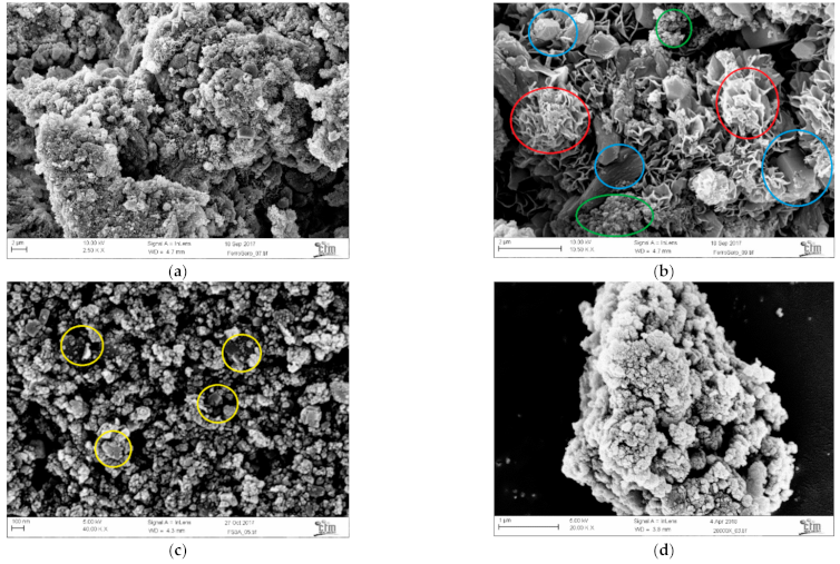
3.1. Characterization of Adsorbents
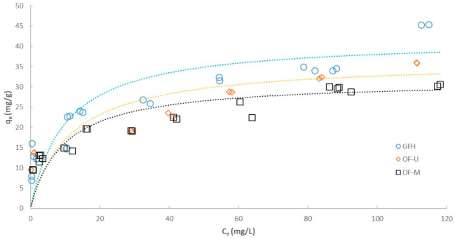
3.2. Effect of Particle Size on Adsorption Isotherm
3.3. Removal of Phosphate from Wastewater
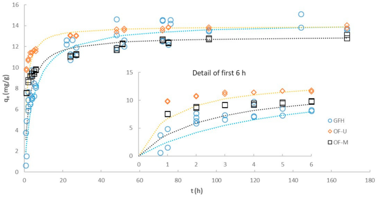
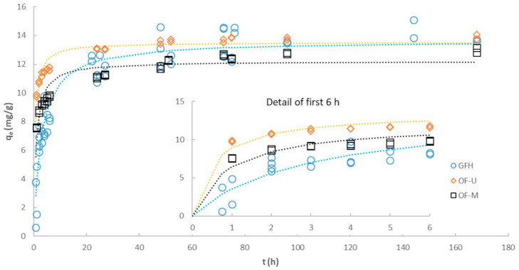
3.4. Effect of Particle Size on Kinetics
4. Conclusions
Supplementary Materials
Author Contributions
Funding
Institutional Review Board Statement
Informed Consent Statement
Data Availability Statement
Acknowledgments
Conflicts of Interest
References
- Genz, A.; Kornmüller, A.; Jekel, M. Advanced phosphorus removal from membrane filtrates by adsorption on activated aluminium oxide and granulated ferric hydroxide. Water Res. 2004, 38, 3523–3530. [Google Scholar] [CrossRef] [PubMed]
- Kalaitzidou, K.; Mitrakas, M.; Raptopoulou, C.; Tolkou, A.; Palasantza, P.A.; Zouboulis, A. Pilot-Scale Phosphate Recovery from Secondary Wastewater Effluents. Environ. Process. 2016, 3, 5–22. [Google Scholar] [CrossRef]
- Yogev, U.; Vogler, M.; Nir, O.; Londong, J.; Gross, A. Phosphorous recovery from a novel recirculating aquaculture system followed by its sustainable reuse as a fertilizer. Sci. Total Environ. 2020, 722, 137949. [Google Scholar] [CrossRef] [PubMed]
- Hermassi, M.; Valderrama, C.; Moreno, N.; Font, O.; Querol, X.; Batis, N.; Cortina, J.L. Powdered Ca-activated zeolite for phosphate removal from treated waste-water. J. Chem. Technol. Biotechnol. 2016, 91, 1962–1971. [Google Scholar] [CrossRef]
- Huang, X.; Liao, X.; Shi, B. Adsorption removal of phosphate in industrial wastewater by using metal-loaded skin split waste. J. Hazard. Mater. 2009, 166, 1261–1265. [Google Scholar] [CrossRef]
- Ren, J.; Li, N.; Zhao, L.; Li, L. Pretreatment of Raw Biochar and Phosphate Removal Performance of Modified Granular Iron/Biochar. Trans. Tianjin Univ. 2017, 23, 340–350. [Google Scholar] [CrossRef]
- López, R.; Antelo, J.; Fiol, S.; Macías-García, F. Phosphate adsorption on an industrial residue and subsequent use as an amendment for phosphorous deficient soils. J. Clean. Prod. 2019, 230, 844–853. [Google Scholar] [CrossRef]
- Edet, U.A.; Ifelebuegu, A.O. Kinetics, isotherms, and thermodynamic modeling of the adsorption of phosphates from model wastewater using recycled brick waste. Processes 2020, 8, 665. [Google Scholar] [CrossRef]
- Letshwenyo, M.W.; Sima, T.V. Phosphorus removal from secondary wastewater effluent using copper smelter slag. Heliyon 2020, 6, e04134. [Google Scholar] [CrossRef]
- Mekonnen, D.T.; Alemayehu, E.; Lennartz, B. Removal of phosphate ions from aqueous solutions by adsorption onto leftover coal. Water 2020, 12, 1381. [Google Scholar] [CrossRef]
- Hermassi, M.; Valderrama, C.; Font, O.; Moreno, N.; Querol, X.; Batis, N.H.; Cortina, J.L. Phosphate recovery from aqueous solution by K-zeolite synthesized from fly ash for subsequent valorisation as slow release fertilizer. Sci. Total Environ. 2020, 731, 139002. [Google Scholar] [CrossRef]
- Kunaschk, M.; Schmalz, V.; Dietrich, N.; Dittmar, T.; Worch, E. Novel regeneration method for phosphate loaded granular ferric (hydr)oxide-A contribution to phosphorus recycling. Water Res. 2015, 71, 219–226. [Google Scholar] [CrossRef]
- Suresh Kumar, P.; Ejerssa, W.W.; Wegener, C.C.; Korving, L.; Dugulan, A.I.; Temmink, H.; van Loosdrecht, M.C.M.; Witkamp, G.J. Understanding and improving the reusability of phosphate adsorbents for wastewater effluent polishing. Water Res. 2018, 145, 365–374. [Google Scholar] [CrossRef]
- Sperlich, A.; Schimmelpfennig, S.; Baumgarten, B.; Genz, A.; Amy, G.; Worch, E.; Jekel, M. Predicting anion breakthrough in granular ferric hydroxide (GFH) adsorption filters. Water Res. 2008, 42, 2073–2082. [Google Scholar] [CrossRef]
- Pepper, R.A.; Couperthwaite, S.J.; Millar, G.J. Re-use of waste red mud: Production of a functional iron oxide adsorbent for removal of phosphorous. J. Water Process Eng. 2018, 25, 138–148. [Google Scholar] [CrossRef]
- Streat, M.; Hellgardt, K.; Newton, N.L.R. Hydrous ferric oxide as an adsorbent in water treatment. Part 3: Batch and mini-column adsorption of arsenic, phosphorus, fluorine and cadmium ions. Process Saf. Environ. Prot. 2008, 86, 21–30. [Google Scholar] [CrossRef]
- Suresh Kumar, P.; Korving, L.; Keesman, K.J.; van Loosdrecht, M.C.M.; Witkamp, G.J. Effect of pore size distribution and particle size of porous metal oxides on phosphate adsorption capacity and kinetics. Chem. Eng. J. 2019, 358, 160–169. [Google Scholar] [CrossRef]
- Asano, T. Water Reuse: Issues, Technologies, and Applications, 1st ed.; McGraw-Hill: New York, NY, USA, 2007; ISBN 9780071459273. [Google Scholar]
- You, X.; Farran, A.; Guaya, D.; Valderrama, C.; Soldatov, V.; Cortina, J.L. Phosphate removal from aqueous solutions using a hybrid fibrous exchanger containing hydrated ferric oxide nanoparticles. J. Environ. Chem. Eng. 2016, 4, 388–397. [Google Scholar] [CrossRef]
- Chittoo, B.S.; Sutherland, C. Column breakthrough studies for the removal and recovery of phosphate by lime-iron sludge: Modeling and optimization using artificial neural network and adaptive neuro-fuzzy inference system. Chin. J. Chem. Eng. 2020, 28, 1847–1859. [Google Scholar] [CrossRef]
- Hand, D.W.; Crittenden, J.C.; Thacker, W.E. Simplified Models for Design of Fixed-Bed Adsorption Systems. J. Environ. Eng. 1984, 110, 440–456. [Google Scholar] [CrossRef]
- Pan, L.; Nishimura, Y.; Takaesu, H.; Matsui, Y.; Matsushita, T.; Shirasaki, N. Effects of decreasing activated carbon particle diameter from 30 um to 140 nm on equilibrium adsorption capacity. Water Res. 2017, 124, 425–434. [Google Scholar] [CrossRef] [PubMed]
- Pan, L.; Takagi, Y.; Matsui, Y.; Matsushita, T.; Shirasaki, N. Micro-milling of spent granular activated carbon for its possible reuse as an adsorbent: Remaining capacity and characteristics. Water Res. 2017, 114, 50–58. [Google Scholar] [CrossRef] [PubMed]
- Hilbrandt, I.; Shemer, H.; Ruhl, A.S.; Semiat, R.; Jekel, M. Comparing fine particulate iron hydroxide adsorbents for the removal of phosphate in a hybrid adsorption/ultrafiltration system. Sep. Purif. Technol. 2019, 221, 23–28. [Google Scholar] [CrossRef]
- Han, J.; Ro, H.M. Interpreting competitive adsorption of arsenate and phosphate on nanosized iron (hydr)oxides: Effects of pH and surface loading. Environ. Sci. Pollut. Res. 2018, 25, 28572–28582. [Google Scholar] [CrossRef]
- Li, N.; Ren, J.; Zhao, L.; Wang, Z.L. Fixed bed adsorption study on phosphate removal using nanosized FeOOH-modified anion resin. J. Nanomater. 2013, 2013, 1–5. [Google Scholar] [CrossRef]
- Ribas, D.; Pešková, K.; Jubany, I.; Parma, P.; Černik, M.; Benito, J.A.; Martí, V. High reactive nano zero-valent iron produced via wet milling through abrasion by alumina. Chem. Eng. J. 2019, 366, 235–245. [Google Scholar] [CrossRef]
- Ribas, D.; Cernik, M.; Martí, V.; Benito, J.A. Improvements in nanoscale zero-valent iron production by milling through the addition of alumina. J. Nanoparticle Res. 2016, 18, s11051–s12016. [Google Scholar] [CrossRef]
- Hu, H.; Li, X.; Huang, P.; Zhang, Q.; Yuan, W. Efficient removal of copper from wastewater by using mechanically activated calcium carbonate. J. Environ. Manage. 2017, 203, 1–7. [Google Scholar] [CrossRef]
- Donskoi, E.; Collings, A.F.; Poliakov, A.; Bruckard, W.J. Utilisation of ultrasonic treatment for upgrading of hematitic/goethitic iron ore fines. Int. J. Miner. Process. 2012, 114–117, 80–92. [Google Scholar] [CrossRef]
- Katircioglu-Bayel, D. Effect of Combined Mechanical and Ultrasonic Milling on the Size Reduction of Talc. Mining, Metall. Explor. 2020, 37, 311–320. [Google Scholar] [CrossRef]
- Fasaki, I.; Siamos, K.; Arin, M.; Lommens, P.; Van Driessche, I.; Hopkins, S.C.; Glowacki, B.A.; Arabatzis, I. Ultrasound assisted preparation of stable water-based nanocrystalline TiO2 suspensions for photocatalytic applications of inkjet-printed films. Appl. Catal. A Gen. 2012, 411–412, 60–69. [Google Scholar] [CrossRef]
- Fiol, N.; Villaescusa, I. Determination of sorbent point zero charge: Usefulness in sorption studies. Environ. Chem. Lett. 2009, 7, 79–84. [Google Scholar] [CrossRef]
- Freundlich, H.M.F. Tiber die adsorption in losungen. Z. Phys. Chem. 1906, 57, 385–470. [Google Scholar] [CrossRef]
- Langmuir, I. The constitution and fundamental properties of solids and liquids. J. Am. Chem. Soc. 1916, 38, 2221–2295. [Google Scholar] [CrossRef]
- Kumar, K.V. Linear and non-linear regression analysis for the sorption kinetics of methylene blue onto activated carbon. J. Hazard. Mater. 2006, 137, 1538–1544. [Google Scholar] [CrossRef]
- Zhang, L.; Du, C.; Du, Y.; Xu, M.; Chen, S.; Liu, H. Kinetic and isotherms studies of phosphorus adsorption onto natural riparian wetland sediments: Linear and non-linear methods. Environ. Monit. Assess. 2015, 187, s10661–s11015. [Google Scholar] [CrossRef]
- Khambhaty, Y.; Mody, K.; Basha, S.; Jha, B. Pseudo-second-order kinetic models for the sorption of Hg(II) onto dead biomass of marine Aspergillus niger: Comparison of linear and non-linear methods. Colloids Surfaces A Physicochem. Eng. Asp. 2008, 328, 40–43. [Google Scholar] [CrossRef]
- Draper, N.R. Applied Regression Analysis/Norman R. Draper, Harry Smith; John Wiley & Sons: New York, NY, USA, 1998; ISBN 0471170828. [Google Scholar]
- Potthoff, R. On the Johnson-Neyman technique and some extensions thereof. Psychometrika 1964, 29, 241. [Google Scholar] [CrossRef]
- Andrade, J.M.; Estévez-Pérez, M.G. Statistical comparison of the slopes of two regression lines: A tutorial. Anal. Chim. Acta 2014, 838, 1–12. [Google Scholar] [CrossRef]
- Fox, J. Applied Regression Analysis and Generalized Linear Models; SAGE Publications: Los Angeles, CA, USA, 2016; ISBN 9781452205663. [Google Scholar]
- Townend, J. Practical Statistics for Environmental and Biological Scientists; Wiley: Chichester, UK, 2002; ISBN 0471496650. [Google Scholar]
- Pepper, R.A.; Couperthwaite, S.J.; Millar, G.J. Value adding red mud waste: Impact of red mud composition upon fluoride removal performance of synthesised akaganeite sorbents. J. Environ. Chem. Eng. 2018, 6, 2063–2074. [Google Scholar] [CrossRef]
- Ilavsky, J.; Barlokova, D. The use of granular iron -based sorption materials for nickel removal from water. Polish J. Environ. Stud. 2012, 21, 1229–1236. [Google Scholar]
- Ghasemi, Y.; Emborg, M.; Cwirzen, A. Estimation of specific surface area of particles based on size distribution curve. Mag. Concr. Res. 2018, 70, 533–540. [Google Scholar] [CrossRef]
- Lalley, J.; Han, C.; Mohan, G.R.; Dionysiou, D.D.; Speth, T.F.; Garland, J.; Nadagouda, M.N. Phosphate removal using modified Bayoxide® E33 adsorption media. Environ. Sci. Water Res. Technol. 2015, 1, 96–107. [Google Scholar] [CrossRef]
- Geelhoed, J.S.; Hiemstra, T.; Van Riemsdijk, W.H. Phosphate and sulfate adsorption on goethite: Single anion and competitive adsorption. Geochim. Cosmochim. Acta 1997, 61, 2389–2396. [Google Scholar] [CrossRef]
- LaGrega, M.D.; Buckingham, P.L.; Evans, J.C. Hazardous Waste Management, 2nd, ed.; McGraw-Hill: Boston, MA, USA, 2001; ISBN 0070393656. [Google Scholar]


| GFH | OF-M | OF-U | |
|---|---|---|---|
| Size 1 (µm) | 500–2000 2 | 0.1–2 | 1.9–50.3 |
| BET Surface Area (m2/g) | 199.7 | 98.4 | 160.2 |
| t-plot Micropore Area (m2/g) | 20.9 | 0 | 4.3 |
| Zeta Potential 3 (mV) | −8.4 ± 2.8 | −9.5 ± 1.0 | −8.4 ± 1.9 |
| Equilibrium pH | 8.59 | 9.41 | 9.43 |
| GFH | OF-M | OF-U | ||
|---|---|---|---|---|
| Freundlich model | ||||
| R2 | 0.8847 | 0.9554 | 0.9263 | |
| KF | (mg1−1/n·(L)1/n/g) | 11.59 | 9.70 | 12.78 |
| n | (-) | 4.00 | 4.30 | 5.28 |
| Langmuir model | ||||
| R2 | 0.9481 | 0.9731 | 0.9358 | |
| qmax | (mg/g) | 41.80 | 31.59 | 36.43 |
| b | (L/mg) | 0.1006 | 0.1051 | 0.0871 |
| GFH | OF-M | OF-U | ||
|---|---|---|---|---|
| Langmuir model CI | ||||
| Slope (1/qmax) | (g/mg) | 0.023925 | 0.031652 | 0.027449 |
| Standard error | (g/mg) | 0.001251 | 0.001177 | 0.002076 |
| d.f. 1 | - | 20 | 20 | 12 |
| t-Student 0.025 | - | 2086 | 2086 | 2179 |
| 1/qmax UCL | (g/mg) | 0.026536 | 0.034107 | 0.031971 |
| 1/qmax LCL | (g/mg) | 0.021315 | 0.029196 | 0.022926 |
| Dichotomous model comparison with GFH | ||||
| b3 UCL 2 | - | - | 0.011198 | −0.001109 |
| b3 LCL 2 | - | - | 0.004255 | 0.008156 |
| Initial Conditions | Fitted Values 1 | Experimental Values 2 | ||||||
|---|---|---|---|---|---|---|---|---|
| Sample | Co (mg/L) | m/V (g/L) | qe (mg/g) | Ce (mg/L) | η (%) | qe (mg/g) | Ce (mg/L) | η (%) |
| MR-1 | 3.1 | 2 | 1.38 | 0.34 | 89.1 | >1.28 | <0.5 | >83.9 |
| MR-1 | 3.1 | 3 | 0.96 | 0.23 | 92.5 | >0.87 | <0.5 | >83.9 |
| MR-2 | 41.6 | 2 | 17.3 | 6.98 | 83.2 | 17.8 | 5.55 | 86.6 |
| MR-2 | 41.6 | 3 | 12.5 | 4.20 | 89.9 | 12.8 | 2.85 | 93.1 |
| GFH | OF-M | OF-U | ||
|---|---|---|---|---|
| Pseudo first-order (linear) | ||||
| R2 | 0.6637 | 0.8764 | 0.7313 | |
| k1 | (h−1) | 0.0189 | 0.0237 | 0.0260 |
| Ln (qe) | (Ln(mg/g)) | 1.796 | 1.302 | 0.796 |
| Initial rate 1 | (mg/g·h) | 0.27 | 0.31 | 0.36 |
| SSerr 1 | 1055 | 931.1 | 1397 | |
| Pseudo second-order (linear) | ||||
| R2 | 0.9915 | 0.9989 | 0.9997 | |
| qe | (mg/g) | 14.28 | 13.02 | 13.96 |
| k2 | (g/mg·h) | 0.0146 | 0.0322 | 0.0660 |
| Initial rate 1 | (mg/g·h) | 2.98 | 5.45 | 12.86 |
| SSerr 1 | 85.17 | 58.33 | 28.29 | |
| Pseudo second-order (non-linear) | ||||
| qe | (mg/g) | 13.66 | 12.21 | 13.52 |
| k2 | (g/mg·h) | 0.0257 | 0.0911 | 0.1437 |
| Initial rate 1 | (mg/g·h) | 4.80 | 13.58 | 26.27 |
| SSerr 1 | 53.34 | 11.47 | 5.88 | |
| GFH | OF-M | OF-U | ||
|---|---|---|---|---|
| Linear second-order model CI | ||||
| Slope (1/qe) | (g/mg) | 0.070023 | 0.076830 | 0.071627 |
| Standard error | (g/mg) | 0.00979 | 0.000492 | 0.000227 |
| d.f. 1 | - | 44 | 26 | 26 |
| t-Student 0.025 | - | 2.015 | 2.056 | 2.056 |
| 1/qe UCL | (g/mg) | 0.071996 | 0.077841 | 0.072095 |
| 1/qe LCL | (g/mg) | 0.068049 | 0.075818 | 0.071160 |
| Dichotomous model comparison with GFH | ||||
| b3 UCL 2 | - | - | 0.009413 | 0.004121 |
| b3 LCL 2 | - | - | 0.004200 | −0.000911 |
Publisher’s Note: MDPI stays neutral with regard to jurisdictional claims in published maps and institutional affiliations. |
© 2021 by the authors. Licensee MDPI, Basel, Switzerland. This article is an open access article distributed under the terms and conditions of the Creative Commons Attribution (CC BY) license (https://creativecommons.org/licenses/by/4.0/).
Share and Cite
Martí, V.; Jubany, I.; Ribas, D.; Benito, J.A.; Ferrer, B. Improvement of Phosphate Adsorption Kinetics onto Ferric Hydroxide by Size Reduction. Water 2021, 13, 1558. https://doi.org/10.3390/w13111558
Martí V, Jubany I, Ribas D, Benito JA, Ferrer B. Improvement of Phosphate Adsorption Kinetics onto Ferric Hydroxide by Size Reduction. Water. 2021; 13(11):1558. https://doi.org/10.3390/w13111558
Chicago/Turabian StyleMartí, Vicenç, Irene Jubany, David Ribas, José Antonio Benito, and Berta Ferrer. 2021. "Improvement of Phosphate Adsorption Kinetics onto Ferric Hydroxide by Size Reduction" Water 13, no. 11: 1558. https://doi.org/10.3390/w13111558
APA StyleMartí, V., Jubany, I., Ribas, D., Benito, J. A., & Ferrer, B. (2021). Improvement of Phosphate Adsorption Kinetics onto Ferric Hydroxide by Size Reduction. Water, 13(11), 1558. https://doi.org/10.3390/w13111558