Numerical Analysis of Flow Behavior in a Rectangular Channel with Submerged Weirs

Abstract

In this contribution, different 3D numerical approaches are applied in order to simulate the behaviour of turbulent flow through a rectangular channel with broad-crested weirs. In addition, water flow velocities, using Acoustic Doppler Velocimetry (ADV) instrumentation, were recorded. Two turbulence quantities are estimated using the laboratory records and were compared with those computed with the Large Eddy Simulation (LES) and Reynolds Averaged Navier–Stokes (RANS) models. Additionally, a quadrant analysis of the laboratory records was carried out. The output of the models presents good agreement with the time-averaged parameters, but is not sufficient for the proper estimation of the turbulence quantities.

1. Introduction

Turbulence in open channel flow is a matter of interest to researchers of many fields, e.g., hydraulics, hydro-mechanics, fluid mechanics, and/or environmental engineering. On the one hand, with the advancement of measuring techniques and devices, numerous research works have been carried out experimentally and numerically regarding open channel flow turbulence [1]. On the other hand, in recent years, a large number of hydraulic problems have been solved using Computational Fluid Dynamics (CFD), above all with the usage of the Reynolds Averaged Navier–Stokes (RANS) techniques. Thus, CFD became a real option to analyse the turbulence behaviour with relatively high values of the Reynolds number. CFD is a field of Fluid Mechanics, which has been previously used only by postdoctoral researchers because of its theoretical complexity and high computational cost. It was a field exclusively for high technology engineering areas such as aeronautics or astronautics [2]. The general purpose of CFD is to deal with the characteristics of the motion of fluids described by fundamental equations, with the usage of numerical algorithms, numerical methods, and computers. Nowadays, and thanks to the rapid development of computational facilities, CFD is becoming increasingly accessible for engineering purposes to solve design-oriented tasks in industry, science, and other engineering fields [3].

Examples of the application of RANS models are summarized below. Kirkgoz et al. [4] tested a round crested spillway using the finite element method and the standard k-ε and k-ω turbulence models. The results of their numerical calculations satisfactorily agreed with the experimental data. Andersson et al. [5] performed a full 3D modelling of water spilling from the reservoir with relatively complex geometry using the volume of fluid method (VoF), and he compared these results with two different turbulence models, namely, the standard k-ε and the SSG model. Ouillon and Dartus [6] performed a numerical simulation of flow behaviour downstream of a lateral structure using the k-$\epsilon$ model. Their study demonstrated that the RANS-based methods present good agreement between modelled water surface elevations and those measured in the laboratory. It also demonstrated that RANS models are useful to analyse sediment transport phenomena downstream of the groyne. A novel multiscale k-$\epsilon$ model for flow in porous media was developed by Kuwata et al. [7], where two sets of equations were solved for multiscale turbulence inside porous media. In this model, the dispersive second moment was algebraically modelled with reasonable accuracy, and when the double averaging is applied to the momentum equation, the dispersive covariance, macroscale and microscale Reynolds stresses appeared. Herrera-Granados and Kostecki [8] applied two- and three-dimensional numerical (RNG) modelling to simulate water flow behaviour over the new Niedów barrage in South Poland. The draining capacity of one of the flood alleviation structures (one ogee weir of the hydraulic structure) for exploitation and catastrophic conditions was estimated and compared with experimental data. The model presented very good agreement with the experimental data.

The turbulence in rivers is complicated even further by geometrical variations such as different bed forms, roughness elements, and vegetation, changes in river cross-section, bends causing secondary motions, confluences associated with strong shear layers and all kinds of human-made structures. In cases with abrupt changes in geometry, the turbulence flow behaviour separates large-scale structures and extensive vortices. In shallow river flow, these vortices often comprise mainly a horizontal two-dimensional motion, but near the structures, they are mostly highly three-dimensional [9]. To estimate these structures, RANS methods are not sufficient, and the usage of more complex modelling is a must as well, as it is also becoming very popular, e.g., the application of Large Eddy Simulations in the analysis of civil and environmental engineering problems. It is necessary to highlight that the application of more complex techniques also implies more computational costs. Nonetheless, LES describes the structure of the turbulent flow in detail up to the viscous subrange of the energy cascade process [10]. Bradbrook et al. [11] demonstrated the the potential of Large Eddy Simulation to investigate periodic aspects of flow at river channel confluences. The authors also demonstrated the dependency of the results on the grid size. Koken and Constantinescu [12] presented a numerical investigation of the flow past a vertical wall obstruction in a flat-bed channel using detached eddy simulation (DES). This study provided a better understanding of the flow physics and dynamics of the coherent structures of large-scale eddies and mechanisms responsible for sediment entrainment around the flow obstruction. Herrera-Granados [13] applied two 3D numerical techniques (RNG and LES) to compute the velocity field downstream of one single sharp groyne in a rectangular channel. This study demonstrated that LES is more appropriate for the computation of turbulence characteristics, but more expensive in terms of computational cost.

Submerged Weirs and Flow Behavior

Submerged weirs are training structures with the function of improving navigability. These structures are also built to improve river stability and ecological conditions and to protect the upstream in-stream infrastructures from scour and erosion [14]. Previous studies attempted to analyse the flow behaviour above such training structures using CFD. Jia et al. [15] carried out a three dimensional numerical model (k-$\epsilon$) to study the fields around a submerged weir and analyse its influence on the helical secondary current. They also validated the results of their numerical analyses with experimental studies. Huang and Ng [16] applied one two-dimensional and one three-dimensional efficient finite element model for free surface and turbulent flow to study the flow in a physical model river bend with and without a submerged weir. They demonstrated that without the weir, the flow in the channel is a typical river bend flow with superelevation, and that there is a secondary flow (zone) at the cross-section that is the same size as the secondary flow at the channel width and water depth. Significant changes in the water surface elevations with and without the weir are found near the weir. Maghsoodi et al. [17] simulated the flow over weirs using the k-ε model as an empirical wall function, and the VOF method with genetic reconstruction scheme was adopted to solve the complex free surface. By comparing the 3D-simulation results with the flume data, it was found that the numerical model output of flow over the weir has sufficient accuracy and is in good agreement with the data from the physical model for different weir geometries. Ban and Choi [18] carried out a highly resolved LES for turbulent surface jets over a submerged weir under flat and deformed bed conditions. The LES results provided thorough statistical descriptions of such flows, and comparisons with available experimental data showed good agreement. They compared two cases: a flat bed and a deformed bed downstream of the weir. It was found that, for the flat bed case, splats or strong diverging flows frequently occur near the reattachment point, where strong sweep events are dominant and contribute significantly to the Reynolds stresses. On the other hand, for the deformed bed case, only weak splats are observed near the reattachment point, and relatively weak sweep events remain in this region.

In this contribution, the Renormalization Group (RNG), the standard k-$\epsilon$ models, and one LES are applied to analyse the turbulence characteristics of a channel with trapezoidal broad crested submerged weirs, where the effect of the vertical contraction was previously studied [19]. The output of the model is compared with the instantaneous velocity records carried out in the laboratory to calibrate and verify the models. The main differences between natural flow behaviour (measured in the laboratory) and the numerical discretization are highlighted.

2. Materials and Methods

2.1. Experimental Works

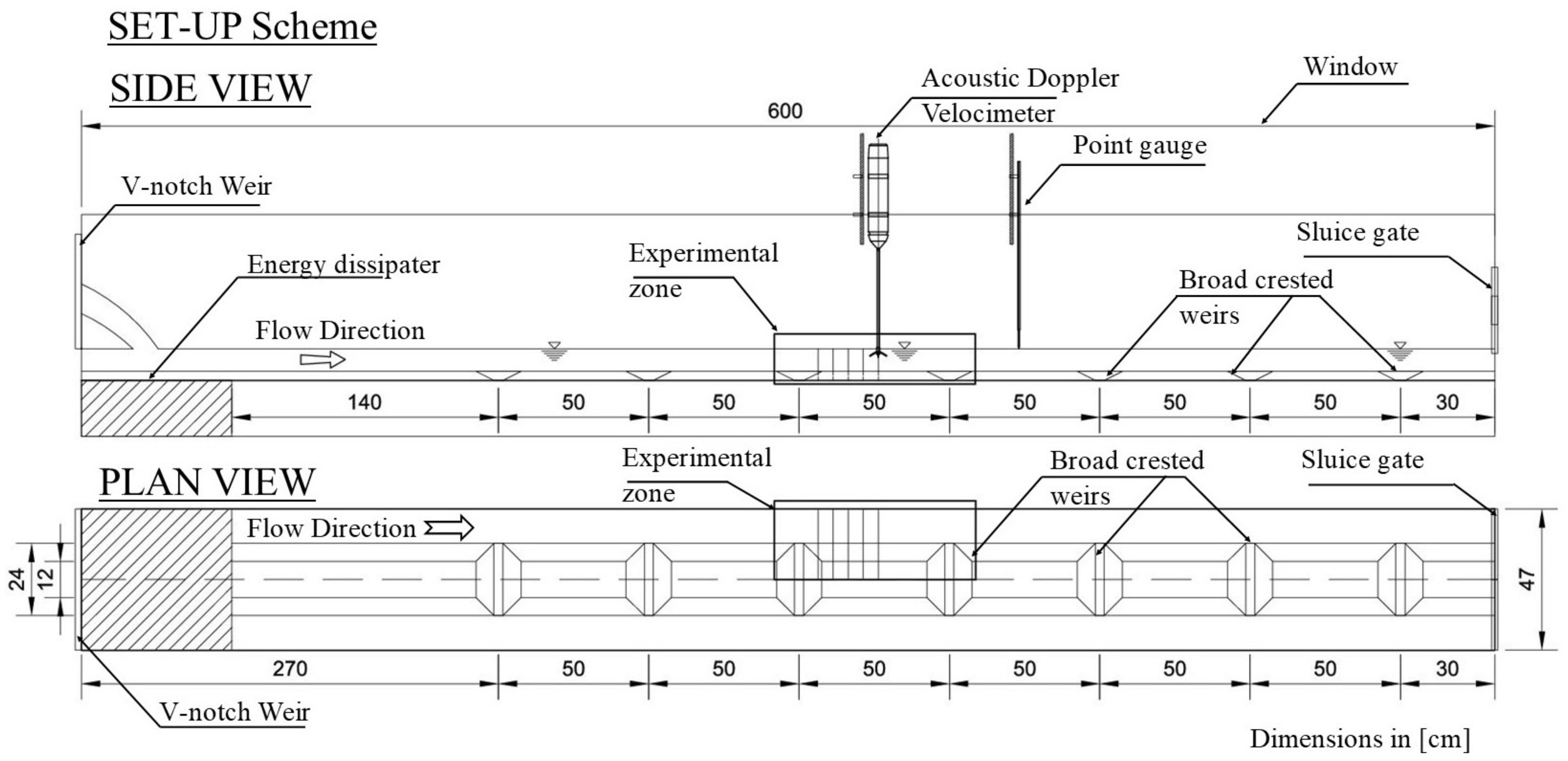
The laboratory research was carried out in a rectangular flume 0.47 m wide, 6.0 m long, and 0.8 m deep. Figure 1 depicts the general layout of the experimental setup as well as the location of the ADV, the point gauge, the trapezoidal weirs, and the structures that control the hydraulic conditions. The Experimental Zone (EZ), where the velocities were registered and recorded, was 0.50 m long, 0.47 m wide, and approximately 0.11 m deep (see Figure 1).

The ADV technique is a widely used tool for the characterization of fluid flow and turbulence. ADVs robustly measure three velocity components within a small sampling volume at high temporal resolution [20]. This technique has been used in a diverse range of applications, due to the fact that the ADV measures at least 5 cm away from its probe tip. Thus, this device can be considered as non-intrusive in most of cases.

The hydrodynamic conditions of the experiments were controlled with a Thomson Weir (upstream) and with a hinged crested gate (downstream). The shallow water flow rate was calculated with the calibrated rating curve of the Thomson weir and with a piezometer indicating the hydraulic head acting on this weir. A flow rate of $Q_e$ = 11.8 dm${}^3$ s${}^{-1}$ was used for the experiments presented in this contribution.

Moreover, the water surface elevation at the end of the channel was measured with a point gauge. For this $Q_e$, the Froude number of the bulk open-channel flow was approximately in the range between 0.20 and 0.40 and the values of the Reynolds number $Re$ were in the range between 15,000 (centre of the main channel) and 25,000 (crest of the weirs). The water surface elevations were measured with a point gauge along the channel and registered from the outlet to the beginning of the flume. The registered hydraulic gradient of the free surface elevation along the experimental zone was approximately 0.001.

2.2. Numerical Modelling—RANS

The 3D dimensional model was based on the modification of the continuity and momentum equations, the commonly used Reynolds-average Navier–Stokes (RANS) equations. In RANS technique, the mean velocity field may be defined by ensemble (time) averaging, which is represented in the following system of equations [21]:

$$\frac{\partial {\overline{u}}_i}{\partial t}+{\overline{u}}_j\frac{\partial {\overline{u}}_i}{\partial x_j}=-\frac{1}{\varrho }\frac{\partial \overline{p}}{\partial x_i}+\nu \frac{{\partial }^2{\overline{u}}_i}{\partial x_j\partial x_j}-\frac{\partial }{\partial x_j}{R}_{ij}$$

(1)

$$\frac{\partial {\overline{u}}_i}{\partial x_i}=0$$

(2)

where ${\overline{u}}_i$ is the mean averaged velocity component, $\overline{p}$ is the mean pressure, $\nu$ is the molecular viscosity, $\varrho$ is the water’s density, and $R_{ij}$ is the kinematic Reynolds stress tensor defined as (3):

$$R_{ij}=-\overline{u_i^{\prime }{u}_j^{\prime }}$$

(3)

where $u_i^{\prime }$ is the fluctuating part of the velocity.

2.3. Turbulence Closures—RANS

Eddy viscosity ${\nu }_T$ plays a profound role in turbulence modelling [10] and it is necessary to properly model the turbulent stresses (see Equation (3)). The Boussinesq approximation is a commonly a way to compute turbulent stresses and it is expressed as:

$$-\overline{u_i^{\prime }{u}_j^{\prime }}={\nu }_T\left(\frac{\partial {\overline{u}}_i}{\partial x_j}+\frac{\partial {\overline{u}}_j}{\partial x_i}\right)-\frac{2}{3}k{\delta }_{ij}$$

(4)

where ${\delta }_{ij}$ is the Kronecker delta and k is the turbulent kinetic energy (TKE) per unit mass, which is defined as follows (5):

$$k\equiv \frac{1}{2}\overline{u_i^{\prime }{u}_i^{\prime }}$$

(5)

In the case of the k-$\epsilon$ model, the eddy viscosity is calculated as:

$${\nu }_T=c_{\mu }\frac{k^2}{\epsilon }$$

(6)

and the TKE is modelled with the following equation:

$$\frac{\partial k}{\partial t}+{\overline{u}}_j\frac{\partial k}{\partial x_j}=\frac{\partial }{\partial x_j}\left(\nu +\frac{{\nu }_T}{{\sigma }_k}\frac{\partial k}{\partial x_j}\right)+P_k-\epsilon$$

(7)

where $P_k$ is the production of turbulence by shear, defined by:

$$P_k=-\overline{u_i^{\prime }{u}_j^{\prime }}\frac{\partial {\overline{u}}_i}{\partial x_j}$$

(8)

and $\epsilon$ is the dissipation rate of k, modelled by:

$$\frac{\partial \epsilon }{\partial t}+{\overline{u}}_j\frac{\partial \epsilon }{\partial x_j}=\frac{\partial }{\partial x_j}\left(\nu +\frac{{\nu }_T}{{\sigma }_{\epsilon }}\frac{\partial \epsilon }{\partial x_j}\right)+c_{\epsilon 1}\frac{\epsilon }{k}{P}_k-c_{\epsilon 2}\frac{{\epsilon }^2}{k}$$

(9)

The terms $c_{\mu }$, ${\sigma }_{\epsilon }$, ${\sigma }_{\epsilon 1}$ and ${\sigma }_{\epsilon }2$ are the constants of the k-$\epsilon$ model.

In the case of the RNG model, this turbulent closure is also part of the RANS technique and it is based on the k-ε technique. The main difference in these two RANS techniques is the way of defining the viscosity. The model constants are the same.

2.4. Large Eddy Simulation

In LES model, the flow variables are decomposed into a large-scale component (or a resolved part), denoted by an overbar, and a subgrid scale (SGS) component. This decomposition is formally achieved by a filtering operation. The resolved part of the field represents the large eddies, while the subgrid part of the velocity represents the small scales whose effect on the resolved field is included through the SGS [13].

The filtering process can be understood as the convolution of a flow variable (in this case velocity) in one dimension $\overline{u}$ is defined by:

$$\overline{u}\left(\mathbf{x}\right)={\int }_{-\infty }^{+\infty }G\left(x,x^{\prime }\right)\overline{u}\left(x^{\prime }\right)d{x}^{\prime }$$

(10)

where $\overline{u}$ represents the resolved part of u and G is the kernel filter depending on the mapping function $x^{\prime }=\left(\mathbf{x}\right)$. Substituting in the decomposition filtering $u=u_i^{\prime }+{\overline{u}}_i$ and $p=p_i^{\prime }+{\overline{p}}_i$ in the Navier–Stokes Equation derives the equations of motion for the resolved field, known as the Filtered Navier–Stokes Equation (FNSE).

$$\frac{\partial {\overline{u}}_i}{\partial t}+{\overline{u}}_j\frac{\partial {\overline{u}}_i}{\partial x_j}=-\frac{1}{\varrho }\frac{\partial \overline{p}}{\partial x_i}+\frac{\partial }{\partial x_j}\left([\nu +{\nu }_{SGS}]\frac{\partial {\overline{u}}_i}{\partial x_j}\right),$$

(11)

where ${\nu }_{SGS}$ is the subgrid-scale turbulent viscosity, equivalent to the eddy viscosity of the RANS model. The most popular SGS model was proposed by Smagorinsky [22]. This model relates the grid size $\overline{\Delta }$ as the length scale (or filter cut-off length scale) to the resolved strain rate $\overline{S_{ij}}$; the ${\nu }_{SGS}$ is modelled by:

$${\nu }_{SGS}={\left(C_s\overline{\Delta }\right)}^2\left|\overline{S_{ij}}\right|$$

(12)

where $\overline{S_{ij}}$ is the rate-of-strain tensor for the resolved scale defined by

$$\overline{S_{ij}}=\frac{1}{2}\left(\frac{\partial {\overline{u}}_i}{\partial x_j}+\frac{\partial {\overline{u}}_j}{\partial x_i}\right)$$

(13)

The filter length is usually calculated as $\overline{\Delta }=V^{1/3}$, where V is the volume of the computational cell. The Smagorinsky $C_s$ constant usually has the value 0.1–0.2. This is the mathematical framework within the Flow3D program [13].

2.5. Numerical Mesh and Boundary Conditions

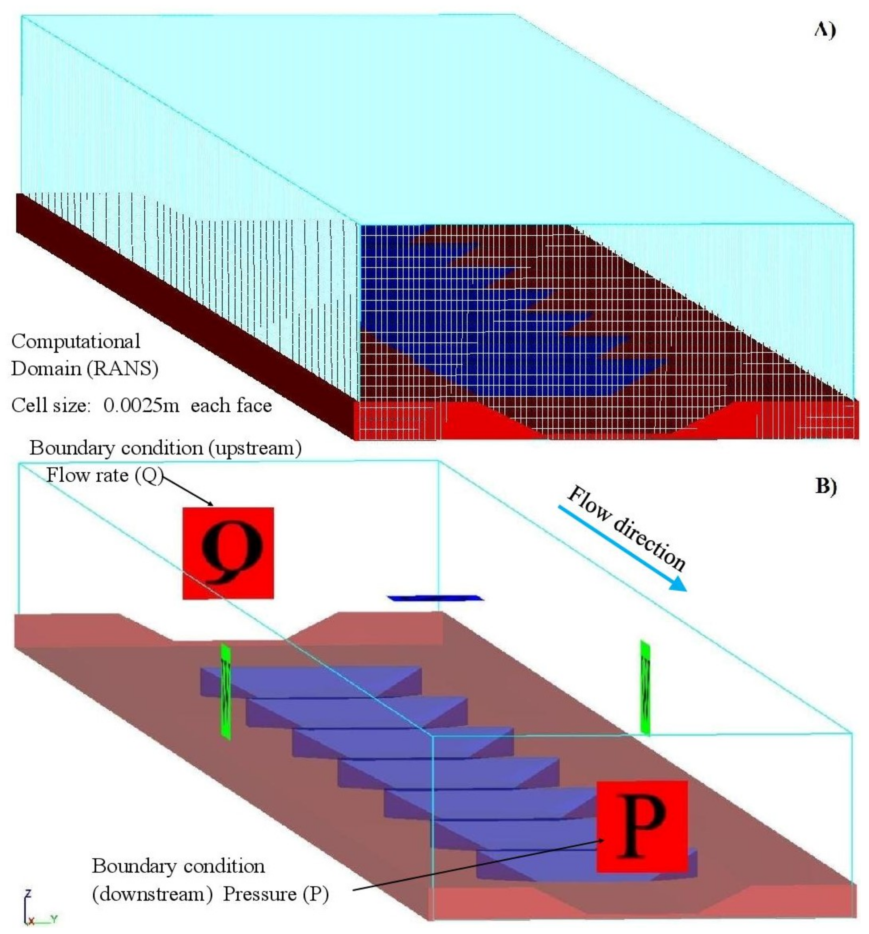
To discretize the RANS equations, the commercially available Computational Fluid Dynamics (CFD) code, Flow3D from Flow Science was used. Flow-3D calculates free surfaces with the VoF method and incorporates a special technique, known as the FAVOR (Fractional Area Volume Obstacle Representation) technique [8] to define general geometric regions within the rectangular grid. The numerical mesh and the FAVOR’ized view of the rectangular channel that were used for the present analysis are depicted in Figure 2A. One numerical hexahedron mesh, built with uniform cubic elements, was used to simulate the water flow along the flume. The size of the computational domain is 4.5 m in the streamwise direction, 0.47 m in the spanwise direction, and 0.12 m in the normal direction with respect to the flume’s bed. The size of the mesh cell was chosen in order that the streamwise velocity profiles can follow the logarithmic law in the centre of the channel in between the trapezoidal weirs.

An additional nested mesh was inserted in the centre of the flume at the location of the experimental zone for the LES. The size of this nested mesh is 0.70 m (length) × 0.25 m (width) and 0.12 m (height). For the LES model, the filter width $\Delta$ is taken to be proportional to the grid size; which should be chosen in such a way that the smallest resolved eddy of size $\Delta$, can be reproduced accurately [13]. Thus, the size of the nested mesh cell is 0.001 m, based on the computations of the previously defined RANS model.

The boundary conditions of the 3D numerical are depicted in Figure 2B. In the upstream side of the flume, the boundary condition was established with the Thomson weir (see Figure 1) and its rating curve, using the same flow conditions as for the experimental works ($Q_e$); this is represented with the letter Q in Figure 2B. In the downstream side, the water level recorded in the laboratory was established as a boundary condition (designated the letter P, or pressure condition, in Figure 2B). In addition, the CFD code provides the option of defining a “S—symmetry” boundary condition, which means that all fluxes at the boundary are equal to zero. This boundary type was used in the top of the mesh, while a nonslip boundary condition was established in the lateral walls.

2.6. Calibration and Validation of the Model

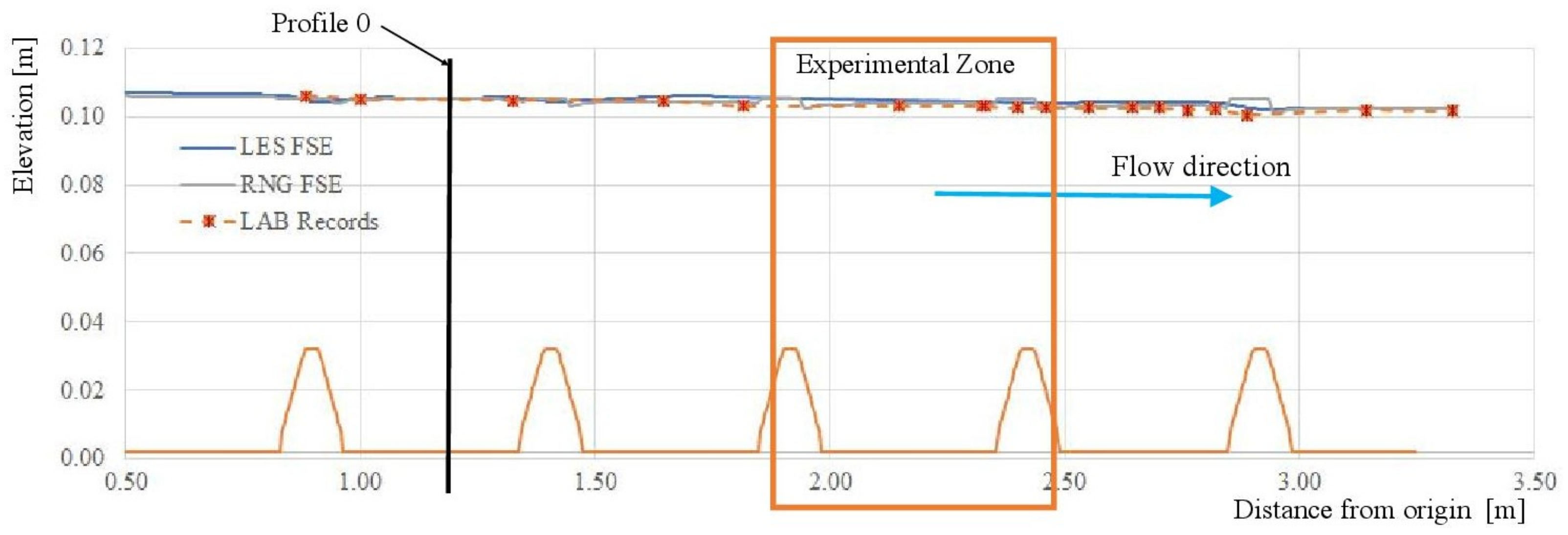
The model was calibrated with the water levels registered with the point gauge in the laboratory (see Figure 3).

As depicted in Figure 3, the model was calibrated comparing the computed values (FSE—Free (water) Surface Elevation) of two of the numerical approaches (output of the LES and the RNG models) with the registered values during the experiments (using the point gauge depicted in Figure 1). The main parameter that was used/modified in the calibration process was the roughness coefficient (Manning n) of the RNG turbulence closure. This model was run several times and once the discrepancy of the output was lower than 2% (compared with the registered values in the laboratory), then the author considered that the model is reliable enough to use other turbulence closures (k-$\epsilon$ and LES). The output of the k-$\epsilon$ model was practically the same in comparison with the output of the RNG model.The results derived from the LES approach are also depicted in Figure 3. It is possible to appreciate that there is not a considerable discrepancy between the output of the FSE (less than 2%) and the registered records in the laboratory.

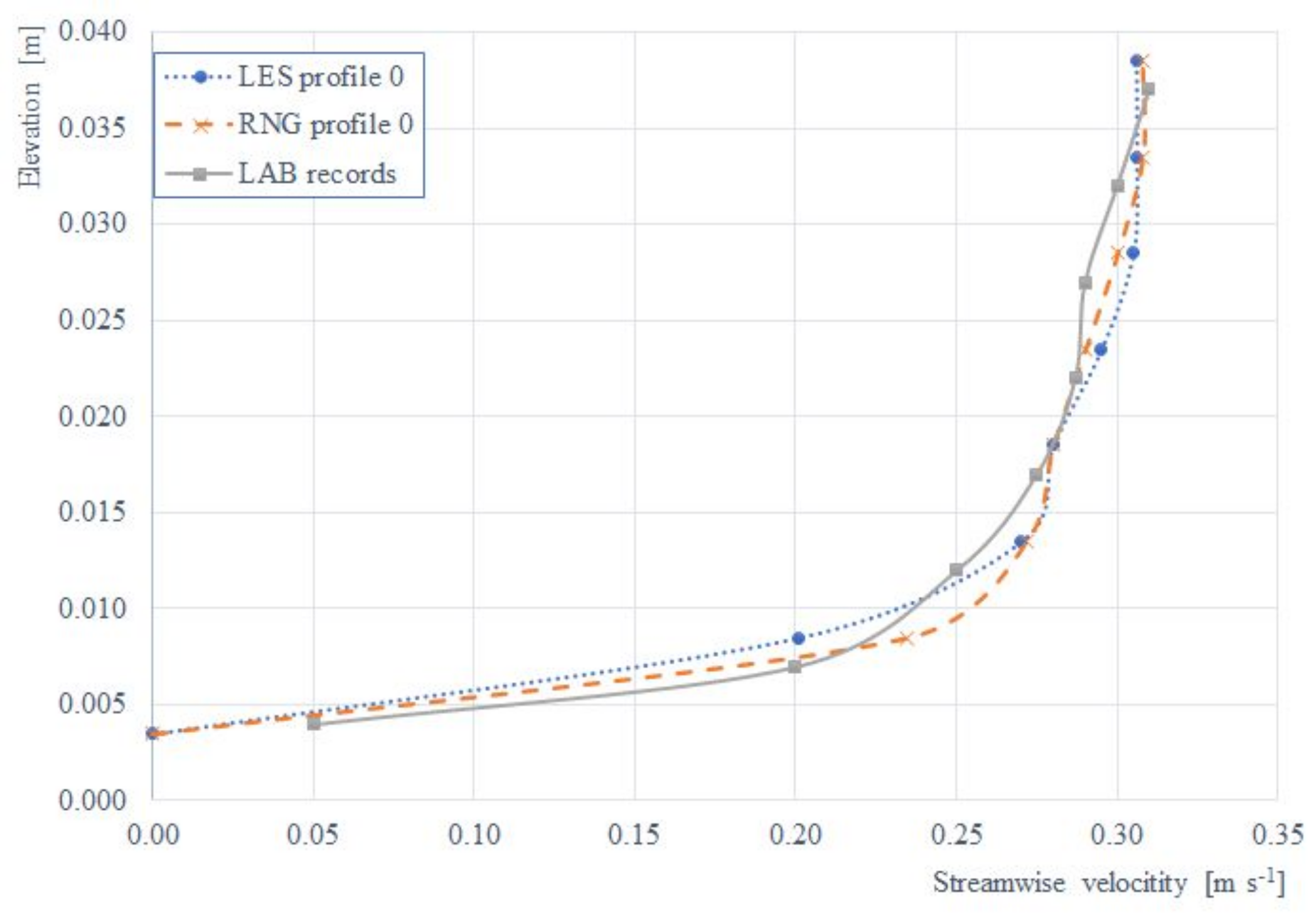
To increase the feasibility of the model, a validation process was also carried out. For this process, the values of the the RNG and LES models were compared with the time-averaged values of the X-velocity profile (downstream direction) at the location of the profile 0 (see Figure 3). The location of the profile 0 assures non-isotropic turbulence disturbances and fulfils the logarithmic law of the wall at this location (see Figure 4). As depicted in Figure 4, the computed (using two different numerical closures) and the registered values are very similar.

3. Results

3.1. Turbulence Bursting

The wall-shear layer of turbulent flow is characterized by a sequence of turbulent events known as the bursting phenomenon. This represents a mechanism of turbulent energy generation near the wall. This phenomenon can be described as a sequence of quasi-cyclic events, where the low-speed fluid streaks are ejected from the near-wall zone, and sweep events, where the high-speed fluid streaks move from upstream toward the wall, sweeping away the slowly moving fluid left from the ejections [23]. The quadrant threshold analysis is a technique that allows detecting the bursting events of the cycle as interactions of two orthogonal components of the instantaneous velocity (u, v, w) in the streamwise x, spanwise y and vertical z directions, respectively, and their fluctuations ($u^{\prime }$, $v^{\prime }$, $w^{\prime }$) in four quadrants of a 2D Cartesian reference (see Figure 5) as follows: outward interactions (Q-I), ejections (Q-II), inward interactions (Q-III) and sweeps (Q-IV). Ejections and sweeps entail quite different flow kinematics, but both contribute to the increase of the absolute magnitude of Reynolds shear stresses [24].

By using the concept of a hyperbolic hole of size H, which is the zone bounded below the curve $\left|u^{\prime }{w}^{\prime }\right|$; the contribution from a particular quadrant can be quantified as [25]:

$${\left(\overline{u^{\prime }{w}^{\prime }}\right)}_{Q,H}=\underset{T\to \infty }{lim}\frac{1}{N}{\int }_0^N{u}^{\prime }\left(t\right)v^{\prime }\left(t\right){\mathrm{\Phi }}_Q\left(t\right)dt$$

(14)

where ${\mathrm{\Phi }}_Q\left(t\right)$ is a detection function defined as:

$${\mathrm{\Phi }}_Q\left(t\right)=\left\{\begin{array}{c}1,\mathrm{when}{\left|u^{\prime }{w}^{\prime }\right|}_Q\ge H{u}_{rms}{w}_{rms}\hfill \\ 0,\mathrm{otherwise}\hfill \end{array}\right.$$

(15)

where $u_{rms}$ and $w_{rms}$ are the turbulent intensities in streamwise and vertical directions, respectively. The parameter H defines a threshold value, which separates the extreme events from the random background turbulence, N is the number of samples, Q is a particular quadrant, and t is the sampling instant. The bigger the value of H, the more extreme strong events are identified [26]. To study the fractional contributions towards the Reynolds shear stresses production from different bursting events, the data of $S_{Q,H}$ equal to $\overline{u^{\prime }{w}^{\prime }}$, normalized by localized Reynolds shear stress is estimated, such as depicted in Figure 6, Figure 7 and Figure 8. The Reynolds shear stress fractional contribution to each event is given by the following equation:

$$S_{Q,H}=\frac{{\left(\overline{u^{\prime }{w}^{\prime }}\right)}_{Q,H}}{\overline{u^{\prime }{w}^{\prime }}}$$

(16)

Figure 6 depicts the quadrant analysis of eight points measured and recorded with ADV in the downstream side close to the toe of the third weir of the flume (see Figure 1 and Figure 9). The legend $Z/Z_o$, represents the location of the test point on the basis of the normalized water depth.

The first profile (PF1 of Figure 9) is located a few millimetres downstream of the toe of the weir and around 2.45 m from the origin of the flume; the second (PF2) and third (PF3) profiles (PF2) are located 5 and 10 cm downstream the first profile PF1, respectively. As depicted in all these figures, Q-II and Q-IV events are dominant in the $XZ$ plane. The presence of sweeps is stronger close to the bottom of the channel, while ejections arise with the water depth. Furthermore, it is observable that the bursting events are stronger close to the weir (PF1) and are getting weaker downstream (PF2 and PF3). The results of the quadrant analyses will be commented within the discussion.

3.2. RANS Modelling

The comparison of the output of the two numerical models is depicted in Figure 9, Figure 10 and Figure 11. Figure 9 depicts the velocity field in x-direction in the $XZ$ plane within the EZ of Figure 1. The output of the RNG and k-$\epsilon$ models is displayed above (A) and below (B), respectively, in all figures. Additionally, in Figure 9, the location of the profiles PF1, PF2, and PF3, which were previously mentioned for the turbulence bursting analyses, is depicted as well.

Regardless the fact that the turbulent closures are very similar (RANS approach), it is possible to observe differences between the models. In Figure 9, the values of u are larger in the zone above the crest of the weirs in the case of the RNG model. In addition, in the output of the RNG model, it is noticeable that the zones with secondary currents seem to be shorter than in the k-$\epsilon$ approach. At the end of the same figure, the velocity vectors indicate that the logarithmic law of the velocity is better computed with the RNG model.

In the case of Figure 10, the RNG model is calculating a broader distribution of the TKE along the space of the two weirs, while the k-$\epsilon$ model is estimating bigger values near the bottom of the channel close to the toe of the first weir. This situation is different when observing the computed contours by the RNG model, where close to the bottom and toe of the trapezoidal weirs (where PF1, PF2, and PF3 are located), the computed values of TKE are smaller than those obtained with the k-$\epsilon$.

A similar situation is observed with the computed turbulent intensity of Figure 11. A broader distribution of the computed values along the space between the weirs can be observed in Figure 11a, which means that the RNG model is able to capture in a clearer way, the turbulence behaviour of the flow within the computational domain while the k-$\epsilon$ model seems to overestimate the turbulence behaviour downstream the location of the toe, where secondary currents arise. In addition, it seems that the model is not able to catch the bursting events that are weaker within the computational domain.

3.3. Large Eddy Simulation

In this subsection, the output of the large eddy simulation is depicted.

In Figure 12 the computed values between the two weirs of the experimental zone are depicted for (A) the mean streamwise velocity; (B) turbulent intensities (%) and the (C) TKE. The y-axis depicts the values of the flume elevation, and the x-axis depicts the values of the distance from the flume’s beginning.

Furthermore, In Figure 13, the computed values between the two weirs of the experimental zone are depicted for (A) the computed turbulent length scale (m) and the (B) vorticity (%) and the (C) TKE. The y-axis depicts the values of the flume elevation and the x-axis depicts the values of the distance from the flume’s beginning.

4. Discussion

The time-averaged velocity profiles $\overline{u}$, observed Reynolds shear stresses in the $XZ$-plane and TKE were estimated by analysing the instantaneous velocity fluctuations of the recorded time series and the output of the numerical models. The Reynolds shear stresses were calculated directly from the velocity fluctuations as follows [27]:

$${\tau }_{xz}=-\rho \overline{u^{\prime }{w}^{\prime }}$$

(17)

while TKE was calculated by:

$$k\equiv \frac{1}{2}\overline{u_i^{\prime }{u}_i^{\prime }}\approx \frac{1}{2}\left(\overline{u^{\prime 2}}+\overline{v^{\prime 2}}+\overline{w^{\prime 2}}\right)$$

(18)

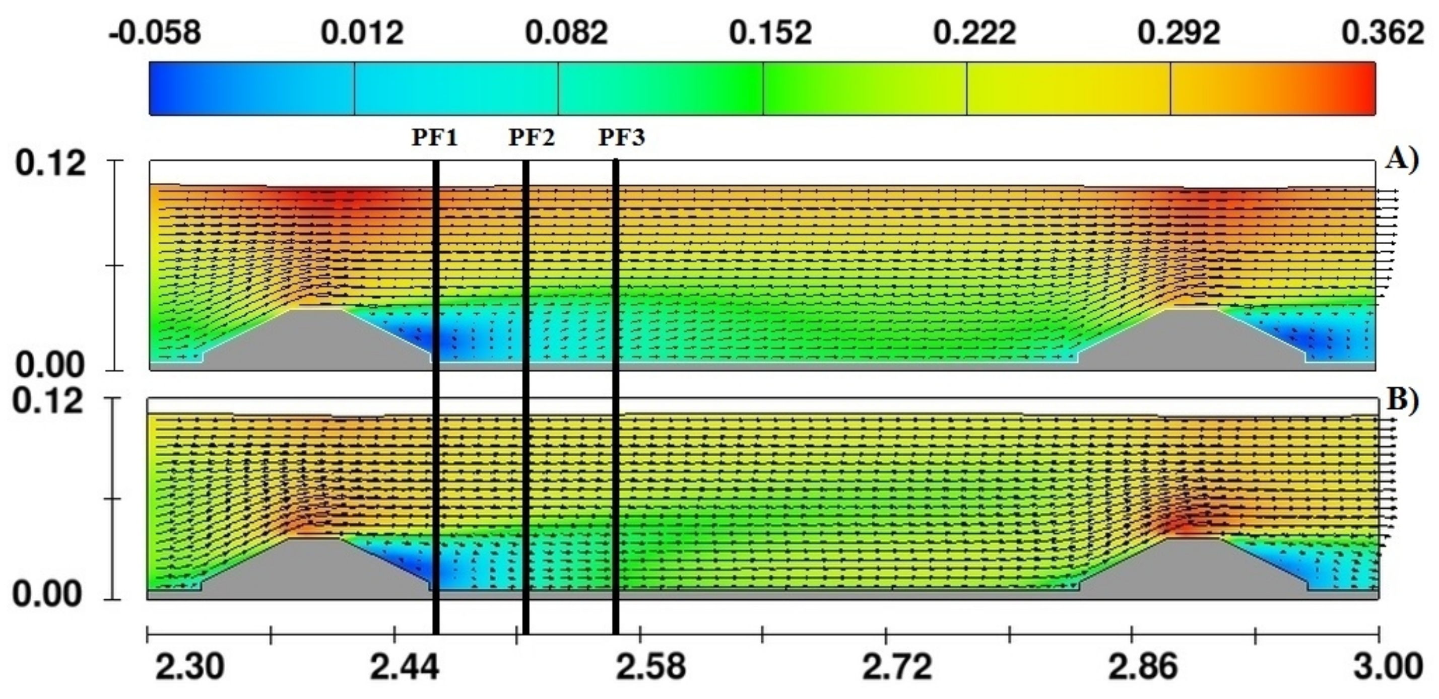
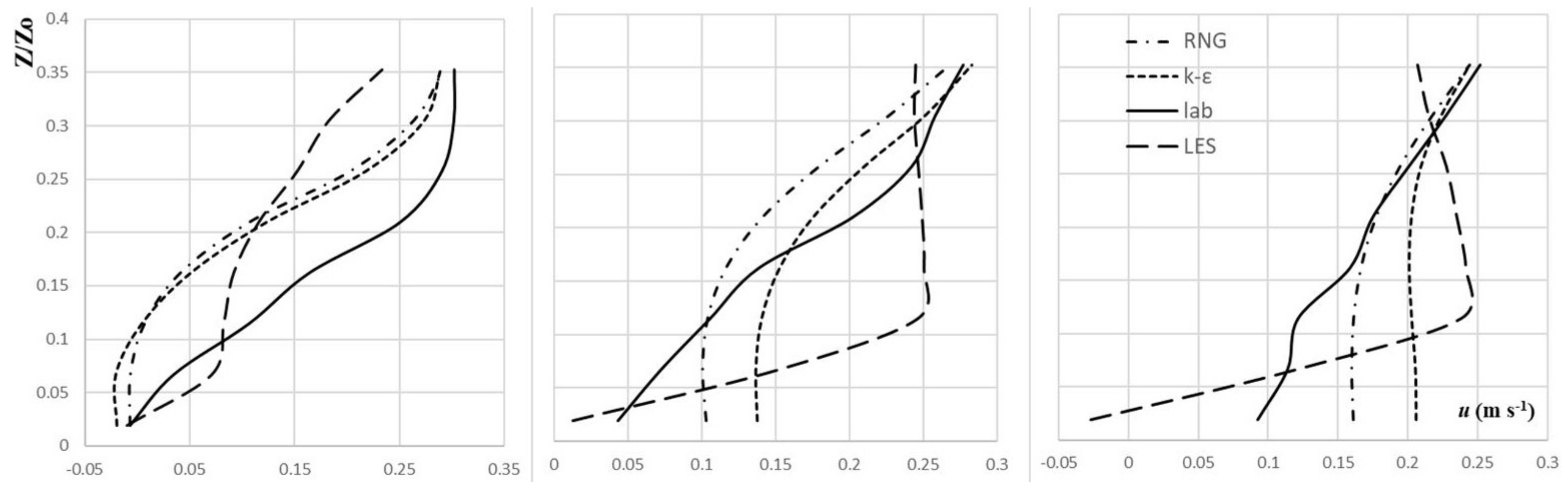
Figure 14 depicts the time-averaged velocity profiles in the streamwise direction in the region close to the bottom of the channel up to $Z/Z_o<$ 0.36.

Below the normalized depth equals of 0.30, the models seem to underestimate the value of u close to the toe of the weir and overestimate it in the zones where secondary currents arise.

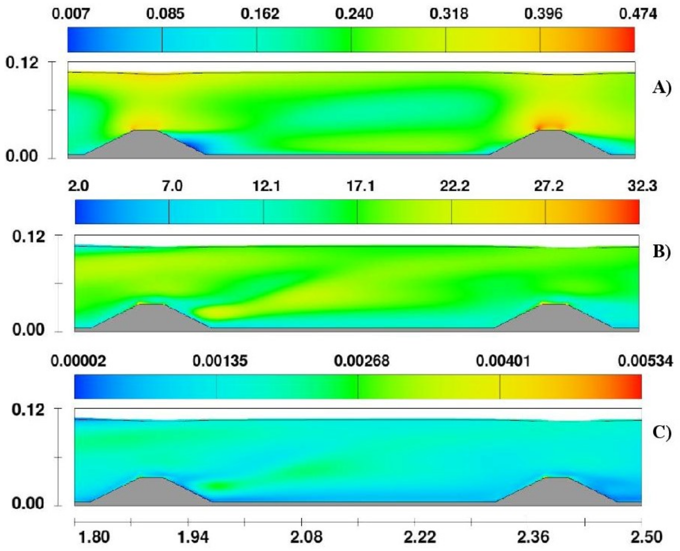
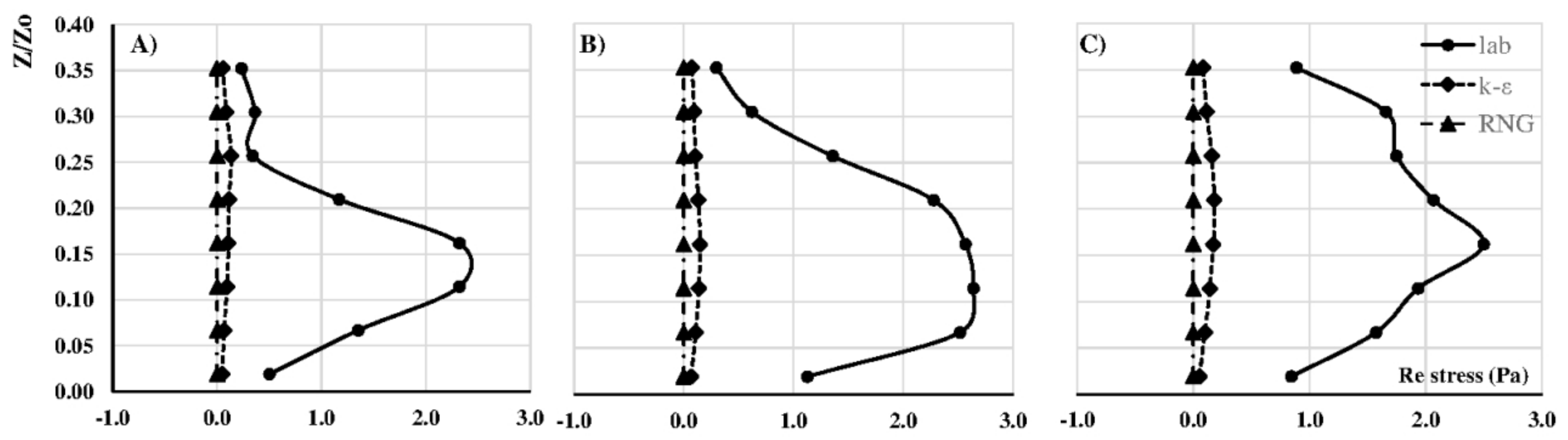
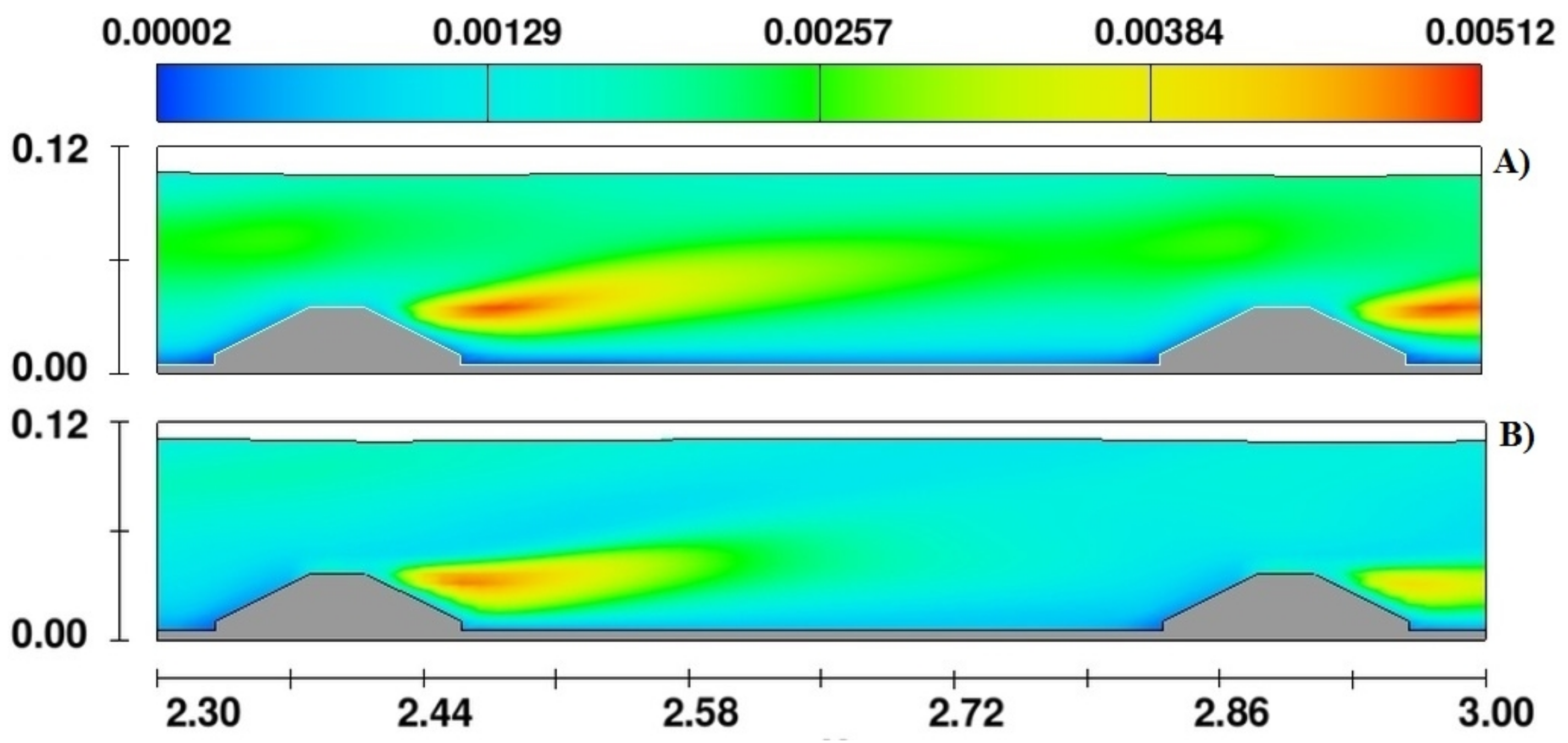
The LES approach seems to capture additional turbulence structures close to the vicinity of the submerged weirs. Something different can be stated observing the comparison of the Reynolds stresses of Figure 15, where both models are underestimating the anisotropic behaviour of the secondary currents and the average values of the computed Reynolds stresses are close to zero (full isotropic behaviour).

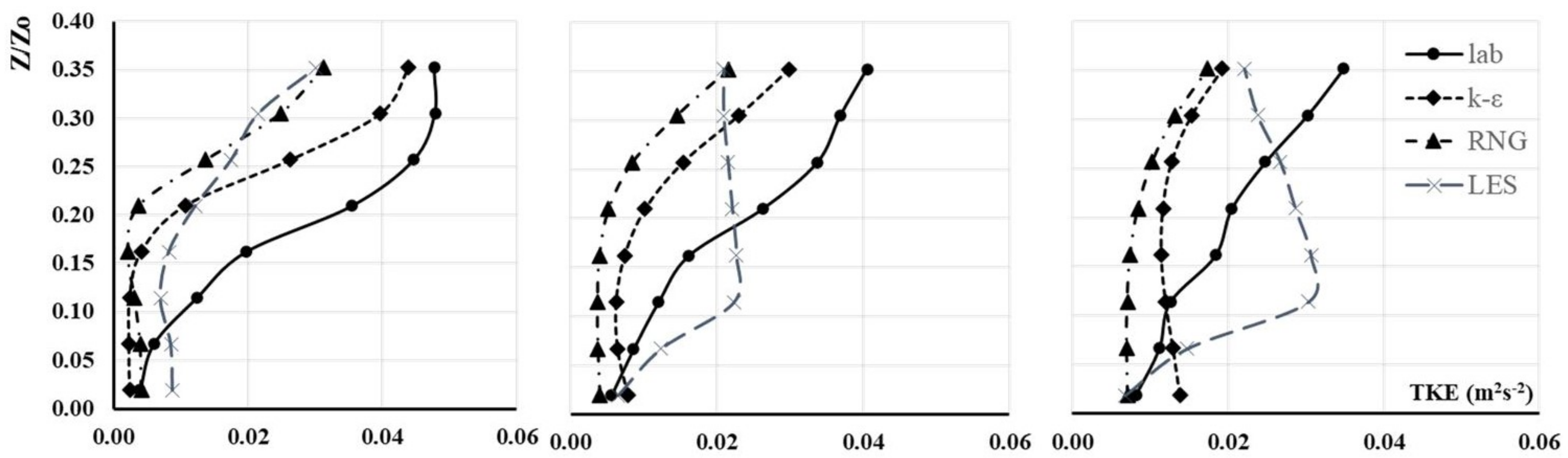
A strange fact occurs with the comparison of the TKE depicted in Figure 16, where the profiles of the k-$\epsilon$ close to the bottom of the channel are overestimated and in the zones of secondary currents are below the registered values in the laboratory. The RNG model is underestimating the values of the TKE in all cases. A possible explanation of this behaviour is that the k-$\epsilon$ approach is overestimating the values of the fluctuations in the spanwise direction.

5. Conclusions

Due to the fact that river flows practically always in the turbulent regime; it is important to understand the flow-structure interaction to increase the reliability of CFD simulations. In the present contribution, full three-dimensional numerical modelling was used to predict the velocity field of a prismatic channel with trapezoidal broad-crested weirs. The laboratory measurements demonstrated that the output of the RNG closure is the most reliable of the RANS techniques to analyse the turbulence behaviour in a channel where the vertical contraction plays a dominant role. As demonstrated, the RNG model predicts more accurately the velocity field downstream of the vertical obstructions, where some turbulent structures can be identified. In the comparison between the laboratory records and the computed values, the k-$\epsilon$ model seems to compute bigger velocity values using the same hydrodynamic and geometric conditions.

The time-averaged velocity profiles and Reynolds stresses in $XZ$ plane, obtained with both RNG and k-$\epsilon$ models, do not differ drastically between each other. On the other hand, the computed TKE profiles of the k-$\epsilon$ model demonstrate that this calibrated model overestimates the values of the TKE in zones with secondary currents. Regardless, both models attempt to account for the different scales of turbulent motion; none of them is able to capture the most important turbulent structures as depicted in Figure 10 and Figure 11. Probably, only the RNG model is able to capture some of the strong bursting events that were estimated in Figure 6, Figure 7 and Figure 8. Thus, the RNG approach seems to be a feasible technique to predict flow behaviour in vertical structures. It can be considered as a proper tool to analyse engineering problems, e.g., sediment transport phenomena on river training structures, such as Ouillon and Dartus [6] demonstrated with a single groyne and the k-$\epsilon$ model, but it is insufficient for complex scientific research. Regardless, the fact is that most of hydraulic engineering projects are still being evaluated with the usage of physical models. CFD modelling represents a cheaper alternative (in terms of budget) to verify the feasibility of river engineering projects. Nonetheless, it is still not sufficient for scientific research (depending on the computer facilities of the analyser). The presented results in this contribution may encourage water specialists to analyse the functionality and design of river infrastructure using CFD. The author is convinced that 3D numerical approaches represent a feasible tool to analyse hydro-engineering problems, but taking into consideration the limitations that these tools can have. Moreover, at the same time, the usage of more appropriate techniques, such as Large Eddy Simulations (LES) or combinations of LES-RAS modelling will be more available for engineering purposes.