Abstract
The purpleback flying squid (Ommastrephidae: Sthenoteuthis oualaniensis) is an important species at higher trophic levels of the regional marine ecosystem in the South China Sea (SCS), where it is considered to show the potential for fishery development. Accordingly, under increasing climatic and environmental changes, understanding the nature and importance of various factors that determine the spatial and temporal distribution and abundance of S. oualaniensis in the SCS is of great scientific and socio-economic interest. Using generalized additive model (GAM) methods, we analyzed the relationship between available environmental factors and catch per unit effort (CPUE) data of S. oualaniensis. The body size of S. oualaniensis in the SCS was relatively small (<19.4 cm), with a shorter lifespan than individuals in other seas. The biological characteristics indicate that S. oualaniensis in the SCS showed a positive allometric growth, and could be suitably described by the logistic growth equation. In our study, the sea areas with higher CPUE were mainly distributed at 10°–11° N, with a 27–28 °C sea surface temperature (SST) range, a sea surface height anomaly (SSHA) of −0.05–0.05 m, and chlorophyll-a concentration (Chl-a) higher than 0.18 μg/L. The SST was the most important factor in the GAM analysis and the best fitting GAM model explained 67.9% of the variance. Understanding the biological characteristics and habitat status of S. oualaniensis in the SCS will benefit the management of this resource.
1. Introduction
Cephalopods are widely distributed in the ocean. They constitute a key group in the marine food web, connecting predators and prey [1]. Cephalopod catches increased from more than 1 million tons in 1970 to 4.3 million tons in 2007 [2], but decreased from 4.03 million tons in 2012 to 3.63 tons in 2018 according to the Food and Agriculture Organization (FAO) yearbook report [3]. Subsequently, the annual cephalopod production was stable, except occasional fluctuations in composition of a few economically important cephalopod species [4]. According to the FAO’s estimation, the total biomass of Sthenoteuthis oualaniensis in the Indian Ocean and Pacific Ocean was between 8 and 11.2 million tons [2]. As an economically important species in the South China Sea, S. oualaniensis is characterized by high fecundity, fast growth and high abundance [5,6,7]. Acoustic survey data inferred that S. oualaniensis resource amount in the open seas of the South China Sea reached 1.5 million tons [8]; the light lure resource assessment model estimated that the total catchable S. oualaniensis in the South China Sea was 994 thousand tons and the resource amount reached 2.05 million tons [9].
The marine environmental conditions have direct impacts on the survival, distribution, replenishment and migration of cephalopods [10]. Understanding the impact of the marine environment on S. oualaniensis is conducive to effective sustainable management of this species [11]. Remote sensing of marine environments is being widely used in the study of sustainable fishery development and fishing efficiency [12,13,14]. Satellite remote sensing can provide large-scale and high-resolution sea environmental information under appropriate conditions [15]. Research has shown that sea surface temperature (SST) was an important indicator of the distribution of marine pelagic fishery resources and changes in the marine environment [16], resulting in a positive correlation between the amount of marine biological resources and SST [16,17,18]. Phytoplankton is an important part of net primary productivity, and could be estimated by chlorophyll-a concentration (Chl-a) from the ocean color data observed by satellites. [11]. Unfortunately, the relationship between Chl-a and resources showed time lags [19]. Satellite remote sensing of sea surface height anomaly (SSHA) data can help identify the changes in ocean current patterns and current velocity (CV) [20]. As it is a complex dynamic process, SSHA cannot directly reflect the distribution of resources like other environmental factors [21].
Analysis of measurement data shows that marine ecosystems are dynamic and nonlinear, and there are obvious problems in empirical analyses based on traditional statistical methods [22]. The generalized additive models (GAMs) method provides an additional choice for the empirical analysis of the spatial–temporal relationship between marine species and their environment; such models take into account nonlinear responses between variables [19,23]. The combination of GAMs and geographic information systems (GIS) has been demonstrated to be suitable for describing marine habitats and explaining the impact of different environmental factors on marine resources [21,24,25]. For GAMs analysis in the application to cephalopods, SST and Chl-a are the main environmental variables that affect resource changes [17,26,27].
In our study, we analyzed the biological information of S. oualaniensis collected monthly in the South China Sea in 2018 to examine the mantle length–body weight relationship and the dynamics of age structure, aiming to construct an optimal growth model. The GAMs method was used to analyze the correlation between the catch data of S. oualaniensis in the South China Sea and the environmental remote sensing data (SST, Chl-a, SSHA and CV), and then to determine the driving factors affecting the large-scale distribution of the population.
2. Materials and Methods
2.1. Catch Data
The catch data of S. oualaniensis were collected in 2018 from the Guangzhou Ocean Fishery Company’s light falling-net fishing boats (Yuesuiyu 30033 and Yuesuiyu 30035) operating in the South China Sea. Two light falling-net fishing boats were used. Each boat was 55 m long and had 622 kw host power, equipped with a net of 90 m height and 300 m outlet circumference, and a total of 700 fish-collection lights (each at 1 kw). The catch data included time, location (latitude and longitude) and production in both abundance and biomass. The area ranged from 9.875° to 16.875° north latitude and 112.375° to 115.875° east longitude (Table 1 and Figure 1). The catch data was averaged according to the spatial resolution of 0.25° × 0.25° to match environmental remote sensing data.

Table 1.
Fishery data collected in the South China Sea in 2018.
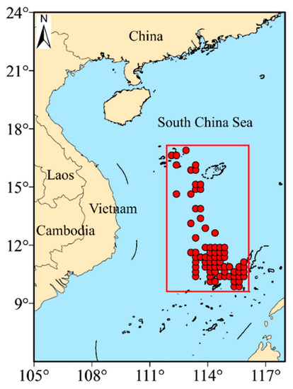
Figure 1.
Station locations available for this study.
2.2. Environmental Remote Sensing Data
Environmental remote sensing data included SST (°C), Chl-a (μg/L), SSHA (m) and absolute geostrophic velocity (AGV, m/s) in the study sea area (9.875°–16.875° N and 112.375°–115.875° E). The AGV includes the zonal component (ZCV) and the meridian component (MCV) for determining a large-scale estimated flow velocity scalar.
The environmental data were from the Pacific node of the Ocean Observation Center of the National Oceanic and Atmospheric Administration (NOAA) in the USA (https://oceanwatch.pifsc.noaa.gov/). The remote sensing data used in the analysis were from the first day of each month in 2018. The spatial resolution of SST was 0.05° × 0.05°; the spatial resolution of Chl-a was 0.0375° × 0.0375°; the spatial resolution of SSHA and AGV was 0.25° × 0.25°. The software ArcGIS (10.2) was used for drawing figures. The calculation equation of current velocity (CV, m/s) was:
2.3. Biological Data
In total, 1387 S. oualaniensis samples from 112.28° E–115.60° E, 10.27° N–16.59° N were provided by the Guangzhou Ocean Fishery Company’s light falling-net fishing boat Yuesuiyu 30,033 in 2018. According to Marine Survey Regulations (GB/T 12763.6-2007), the biological parameters as mantle length and body weight were measured. The mantle length measurement was accurate to 0.1 cm, and the body weight measurement was accurate to 0.01 g.
In the experiments, a knife was used to remove the statoliths in the statocyst, and the statoliths were placed in centrifuge tubes containing 75% alcohol for the statolith grinding experiments. A total of 180 samples were collected and successfully grounded in the statolith grinding experiment. The statolith grinding experiment comprised embedding, grinding, polishing, photographing, and reading and counting the ring patterns [28]. The embedding was carried out with a 1:1 ratio of acrylic powder and hardener and the grinding was carried out 24 h after embedding. Baikalox 0.3 CR alumina polishing powder (Baikalox CR, Baikowski, France) was used for polishing and the photos were taken under an Olympus BX53 microscope (Olympus, Tokyo, Japan) with an Olympus DP26 camera (Olympus, Tokyo, Japan). Each statolith sample was counted separately by two people and one red dot was marked every ten rings (Figure 2). The average values were taken using a criterion of <10% error. Otherwise, a third person calibrated the reading [29].

Figure 2.
Ring counts and measurements of S. oualaniensis statoliths. This sample was collected in September, and was a female S. oualaniensis with a mantle length of 9.8 cm, a body weight of 29.39 g and an age of 62 days. The distance from the core to the longest edge was 118 μm.
2.4. Methods
A power function relationship was established between mantle length and body weight:
Here, BW is body weight in g, ML is mantle length in cm, a (intercept) is an estimated parameter related to the habitat. Parameter b (slope) reflects the growth type: b = 3 means uniform growth; b < 3 means negative allometric growth; b > 3 indicates positive allometric growth [30,31].
Based on the suggestion that one ring represents one day of growth, seven growth model equations were established [28], including linear, exponential, power function, logarithmic, logistic, Gompertz and Von Bertalanffy growth equations.
Logistic growth model equation:
Gompertz growth model equation:
Von Bertalanffy growth model equation:
Here, K is the estimated growth parameter, t0 is the initial age, L∞ is the limit of mantle length, Lt is the mantle length at age t, and t is the age in days.
Akaike’s Information Criterion (AIC) measures the advantages and disadvantages of model fitting. The smaller the AIC value, the better the model fit [32]. The maximum likelihood estimates and model AIC values could be calculated as follows using the planning and solving function in Excel [33]:
Here, o is the observed value, p is the predicted value, and σ is the standard deviation representing 15% of the average observed value. In our study, σ was 17.8 mm.
The catch per unit fishing effort (CPUE, kg/net) is calculated according to the following equation:
Here, Yield is the total catch in the sea area of a 0.25° × 0.25° grid cell, and fishing times are the total number of operations in each grid cell.
The generalized additive models (GAMs) method was used to determine the effects of environmental factors (depth, SST, Chl-a, SSHA and CV) and spatiotemporal factors (month, longitude and latitude) on the ln(CPUE) of S. oualaniensis in the South China Sea. GAMs method generalizes linear regressions by regarding linear functions as covariates [34]. The MGCV package in the R language (Version 4.0.0) was used for GAMs analysis [35,36]. The non-parametric GAMs function is
Here, ln(CPUE) is the logarithmic transformation of the CPUE of S. oualaniensis, g is the connection function and s is a smoothing function.
According to the explanatory power of the model based on single factor, factors were added to the model from large to small in turn. The variables suitable for the model were screened by factor significance, Akaike information criterion (AIC) and generalized cross-validation (GCV) values so as to select the best fitting model.
Each grid cell in different months was considered as a unit for calculating the average CPUE. The environmental factors were grouped to calculate the average CPUE at each scale. The group scale of SST, Chl-a, depth, SSHA, and CV was 1 °C, 0.05 μg/L, 500 m, 0.05 m, and 0.1 m/s, respectively. The most suitable environmental range was determined according to the relationship between CPUE and each environmental factor.
3. Results
3.1. Temporal and Spatial Changes in Environmental Conditions
The SST gradually increased from south to north from January to May and from October to November in the study area. In contrast, from June to September, SST gradually decreased from south to north (Figure 3A); Chl-a did not undergo significant spatial changes during most months, but from July to September, Chl-a in the southern sea area was clearly greater than in the northern sea area with the boundary at 14° N (Figure 3B). In February, November and December, the SSHA in the middle of the study area was relatively high; in September and October, the SSHA was highest to the south of 12° N (Figure 3C).
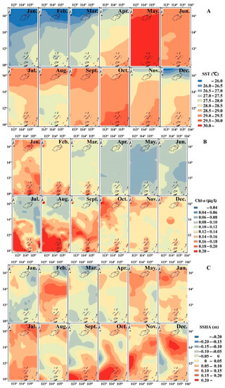
Figure 3.
Spatio-temporal distribution of environmental conditions, including (A): sea surface temperature (SST); (B): Chl-a (chlorophyll-a concentration); and (C): sea surface height anomaly (SSHA).
3.2. Growth Status of S. oualaniensis in the South China Sea
The sample mantle lengths ranged from 7.5 to 19.4 cm with the mean value at 12.3 cm. The monthly mean maximum value appeared in October at 13.5 cm, followed by May at 13.0 cm, November at 12.6 cm and August at 12.5 cm. The smallest average was in December at 11.3 cm (Figure 4).
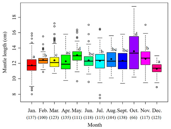
Figure 4.
Monthly variation of mantle length of S. oualaniensis. The black points are the mean values; the white points are the outliers; the thick horizontal lines are the medians; the thin horizontal lines are the upper and lower limits; the rectangles contain the middle 50% of the values. The data below the month represent the samples in number. Different letters means significant differences.
The sample body weights ranged from 10.5 to 302.8 g with the mean value at 76.96 g. The monthly average body weight was highest in October at 107.39 g, followed by May at 89.85 g, August at 86.07 g, September at 80.91 g, and November at 80.57 g. The lowest value appeared in December at 51.97 g (Figure 5).
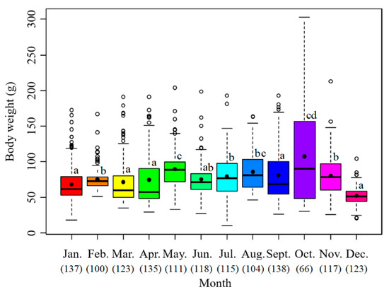
Figure 5.
Monthly variation of body weights of S. oualaniensis. The black points are the mean values; the white points are the outliers; the thick horizontal lines are the medians; the thin horizontal lines are the upper and lower limits; the rectangles contain the middle 50% of the value. The data below the month represent the samples in number. Different letters means significant differences.
A power function relationship between mantle length and body weight of the 1387 S. oualaniensis individuals in the South China Sea in 2018 was established as BW = 0.010ML3.498 (R2 = 0.910), where the b value was greater than three, indicating positive allometric growth (Figure 6).
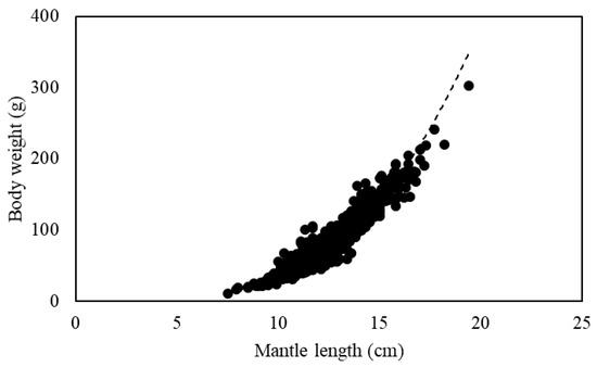
Figure 6.
Relationship of mantle length and body weight of S. oualaniensis.
The age of the oldest individual was 90 days with a mantle length of 15.4 cm and the youngest individual was 45 days old with a mantle length of 8.4 cm. The dominant age range was 50 to 80 days, accounting for 92.7% of the total (Figure 7). The average mantle length of S. oualaniensis was 9.5 cm in the range of 50–59 days, 12.0 cm in the range of 60–69 days, and 13.5 cm in the range of 70–79 days. Within the dominant age group, the S. oualaniensis grew about 2.0 cm every 10 days.

Figure 7.
Frequency distribution of daily age of S. oualaniensis. The numbers in the doughnut diagram indicate the number of samples.
Fitting the optimal growth model based on the statolith ring pattern, the logistic growth equation was the most suitable (AIC = 1199.549). The difference between logistic and AIC values of the Gompertz, von Bertalanffy and power growth equations was about 0.1, while the difference between logistic and logarithmic growth equations was 112.927 (Table 2), thus the logarithmic equation was excluded for describing the growth of S. oualaniensis.
Table 2.
Model equation parameters for S. oualaniensis. Bold means the parameters of the best model.
3.3. Temporal and Spatial Changes in CPUE
The CPUE in the study area showed significant spatial variation. The CPUE range of 74 grid cells was 6.66–741.69 kg/net, with the average value at 195.77 kg/net. The high CPUE were mainly distributed at 10–11° N, and the lower CPUE mostly appeared to the north of 13° N. The pattern of CPUE changes in the longitude direction was unclear (Figure 8).

Figure 8.
Spatial variation of catch per unit effort (CPUE) of S. oualaniensis.
3.4. GAMs Analysis
Starting from the month with the highest interpretation bias, environmental variables were added in turn to the GAMs, and the performance of the model according to AIC and GCV was used to determine which factor was suitable for inclusion in the optimal model. Finally, model 5 with resolution rate was 62.6% was selected as the optimal model, including the following factors: month, SST, SSHA, Chl-a, and latitude resolute (Table 3).
Table 3.
Analysis of variance for generalized additive model (GAMs) fitted to ln(CPUE). Bold means the best model.
In GAMs analysis, month had a positive effect on CPUE from February to June and a negative effect in January. SST had a negative effect on CPUE in the range of 28.0–30.3 °C but a positive effect at other ranges of temperature. SSHA showed a situation where negative and positive effects occurred alternately, with a small effect in the SSHA range of −0.05–0.07 m and a heavy effect when SSHA was higher than 0.07 m. Chl-a higher than 0.18 μg/L showed a positive effect on CPUE but non-significant effects at other values. Latitude had a positive effect on CPUE in the range of 10.0–15.6° and a negative effect at other values (Figure 9).
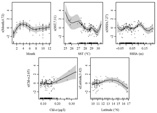
Figure 9.
GAMs analysis of the effects of spatial–temporal and environmental factors on CPUE. The gray shading indicates 95% confidence intervals.
3.5. Relationship between CPUE and Environment
The SST in the study sea area was 25–31 °C and the CPUE was higher in the temperature range of 27–28 °C. The CPUE was higher when Chl-a was greater than 0.18 μg/L. The range of SSHA in the study area was −0.1–0.25 m, in which −0.05–0.05 m was suitable for higher CPUE (Figure 10).

Figure 10.
Relationship between CPUE and environmental factors. “High” and “low” CPUE are defined according to the CPUE conditions of each environment combined with GAM model results.
4. Discussion
4.1. S. Oualaniensis Population Structure
The individual sizes of S. oualaniensis varied in different regions, with the largest individuals caught in the Arabian Sea and the smallest in the South China Sea. For example, the mantle length of S. oualaniensis from the tropical eastern Pacific ranged from 14.2 to 29.7 cm [37]; the mantle length of S. oualaniensis from the southwest and southeast waters of the Arabian Sea in the Indian Ocean was 10.6–61.2 cm and 9.1–27.0 cm, respectively [38,39]; the mantle length of S. oualaniensis from the South China Sea ranged from 5.6 to 23.6 cm [40]. In our study, the mantle length of S. oualaniensis from the South China Sea varied from 7.5 to 19.4 cm, with an average mantle length of 12.3 cm and a median mantle length of 12.2 cm. The individuals of S. oualaniensis in the South China Sea are small, which may be caused by differences in geographic environments and habitats [41]. The open waters of the South China Sea are oligotrophic areas, characterized by lower chlorophyll and lower primary productivity than other sea areas [42]. Individuals of S. oualaniensis in the South China Sea may not obtain enough energy for vertical migration and growth, so the individuals are smaller than those in other sea areas. Oceanic cephalopods can move up a trophic level as mantle length increases from 1.5 to 4.7 cm, suggesting differences in feeding status between individuals of different sizes [43]. The feeding situation of S. oualaniensis varies at different stages of its ontogeny. As the mantle length increases, the feeding changes from zooplankton to crustaceans and lantern fish, and then to lantern fish and cephalopods [44]. According to the concepts of optimal foraging theory [45], during the foraging period, animals should spend the lowest amount of energy and reap the greatest benefits in order to maximize their adaptation to the environment [45].
The b value in the power function relationship between mantle length and body weight reflects the growth status and type of species [46], and the growth type and speed may be different at different developmental stages [47]. The b value is mainly affected by the growth environment of the species and the abundance of food organisms, and the number of samples and the size range can improve the accuracy of the relationship between body length and body weight. Positive allometric growth species tend to inhabit high primary productivity sea areas, while negative allometric growth species tend to inhabit both low primary productivity and deep-sea areas [48]. In our study, the b value 3.498 of S. oualaniensis was consistent with the result 3.367 of samplings from the southern part of the South China Sea (SCS) [49], while the b-value 2.67 in the Indian Ocean waters showed a negative allometric growth type [39]. The ranges of b-values in the Northwest Indian Ocean and South China Sea were 2.584–2.912 and 3.416–3.556, respectively. Individuals in the Indian Ocean were larger and the growth rate of body weight was decreasing compared with the growth rate of mantle length. The individuals in the South China Sea were smaller and their body weights increased rapidly. Different growth types appeared in the two sea areas, which may be due to differences in growth caused by different habitats and food items.
4.2. Analysis of Growth Status of S. oualaniensis
Like most oceanic cephalopods, S. oualaniensis is characterized by rapid growth, efficient reproduction and a short life span [7,50]. According to the statolith ring patterns, the life span mostly ranged from 88 to 363 days [51,52]. The lifespan of S. oualaniensis in the equatorial waters of the eastern Pacific Ocean is about six months; the maximum age is 168 days and the maximum mantle length is 29.6 cm [37]. In our study, the dominant age group of S. oualaniensis from the South China Sea ranged from 50 to 80 days, with the maximum age 90 days and the mantle length of 15.4 cm, indicating that the lifespan of S. oualaniensis in the South China Sea was shorter than those in other seas. This difference in lifespan of S. oualaniensis may reflect the impact of food availability and temperature [53]. Without collecting larvae and juveniles, it was impossible to fully describe the entire growth cycle of S. oualaniensis in the South China Sea. The ontogeny of squid growth in the developmental stage conformed to a linear growth equation and the growth throughout the lifespan generally followed different nonlinear growth models [54,55]. In our study, which only represented adult S. oualaniensis in the South China Sea, the Logistic growth equation was most suitable to describe the growth pattern, consistent with the samplings from the East Pacific [54]. This may be related to the similarity in both sample sizes and developmental stages. Linear and power function growth equations were also considered to be the suitable growth equations for S. oualaniensis in other sea areas [37,56]. Furthermore, except the Logarithmic growth equation that was unsuitable for describing the growth, the AIC values of the other growth models had little difference.
The growth status of S. oualaniensis varied from month to month. Squid have a short lifespan and their growth rate can respond very quickly to changes in ocean conditions [57]. The surface temperature of the South China Sea from May to July was relatively high and Chl-a was relatively low, which resulted in a low primary productivity. S. oualaniensis is a species that spawns throughout the year with the peak spawning time in spring [57]. The maturation peak of female S. oualaniensis mainly occurs in winter, and the individual dies immediately after laying eggs [58].
4.3. Relationship between CPUE and Environment
The spatial variation of the CPUE of oceanic cephalopods with latitude is mainly manifested through temperature changes [59]. In our study, the sea area with higher CPUE was near the Spratly Islands. In the open ocean, Chl-a in the sea area near the islands is relatively high, suggesting primary productivity and abundant food [60]. Oceanic cephalopods likely gather near islands for reproduction, resulting in higher values of CPUE [61].
The marine environment is complex and there are certain connections between various environmental factors [62,63]. Temperature is one of the main factors affecting the growth of organisms. Both low temperature and high temperature will affect the growth of organisms [64,65]. With the increase in SST and the expansion of the hypoxic zone, Chl-a decreased, leading to changes in squid behavior and distributional range [66,67]. In spring, S. oualaniensis was mainly distributed in the SST range of 26.5–28.5 °C in the central and northern waters of the South China Sea [17,19]. According to the GAM analysis for the northeastern part of the Arabian Sea from December to January, the high densities of squid were in the SST range of 28.03–28.62 °C [27]. Based on the habitat suitability index (HSI) model combined with CPUE, the optimal SST range of S. oualaniensis in the South China Sea was 27.4–30.7 °C [68]. For the distant catch of S. oualaniensis, the optimum SST was in the range of 26–28 °C from September to March [69]. There were differences in the optimal SST ranges between different sea areas and seasons. In our study, CPUE was higher when SST was in the range of 27–28 °C. Within the suitable temperature range, CPUE was positively correlated with temperature. Moreover, S. oualaniensis has a wide distribution and vertical migration [61,70], showing a certain degree of adaptability to temperature.
SSHA reflects the dynamic changes of a marine environment, including the current flow velocity and the occurrence of whirlpools. Based on the analysis of the habitat suitability index (HSI) model, the optimal SSHA range of S. oualaniensis from the South China Sea is 0.03–0.18 cm [68]. The edge of a whirlpool was more conducive to the foraging of marine predators such as squid [71]. In our study, the CPUE of SSHA was higher in the range of −0.05–0.05 m. Under GAM analysis, the SSHA range of −0.05–0.07 m had less impact, while a value greater than 0.07 m had a greater impact. Although S. oualaniensis showed a strong swimming ability [72,73] and adaptability to a large range of ocean dynamics, higher SSHA and flow rates were not suitable for the accumulation of bait organisms [71].
Chl-a is an important factor in determining net primary productivity (NPP) by controlling the growth of phytoplankton. Therefore, Chl-a was an important indicator for maintaining the stability of a squid population’s food web structure [13,74,75]. In the southeastern part of the Arabian Sea, the area with the most abundant S. oualaniensis appeared in the Chl-a range of 0.4–0.6 μg/L [27]. A study in the Xisha waters of the South China Sea showed that S. oualaniensis was mainly distributed in sea areas with Chl-a ranging from 0.11 to 0.15 μg/L [17]. In our study, CPUE was higher in areas with Chl-a higher than 0.18 μg/L, consistent with the results of the SCS study [17].
The results of our study show that CPUE was higher when SST was in the range of 27–28 °C, Chl-a > 0.18 μg/L and SSHA in the range of −0.05–0.05 m. According to the analysis on suitable habitat conditions for S. oualaniensis, the suitable period for SST, Chl-a and SSHA was, respectively, in February and March, from July to next March, and from January to March.
5. Conclusions
The purpleback flying squid (Ommastrephidae: Sthenoteuthis oualaniensis) is an important species with potential for resource exploitation in the South China Sea (SCS). Understanding the biological characteristics and habitat status of S. oualaniensis in the South China Sea will aid in the management of this resource.
The body size of S. oualaniensis in the SCS was relatively small, with a shorter lifespan than individuals in other seas. S. oualaniensis in the SCS showed a positive allometric growth, with the relationship between mantle length (ML) and body weight (BW) as BW = 0.010ML3.498 (R2 = 0.910). The dominant age of S. oualaniensis in the SCS was 50–80 days, and the growth model could be better described by a logistic growth equation based on the statolith ring pattern.
To obtain a higher CPUE of S. oualaniensis, a favorable habitat environment was required, including a sea surface temperature (SST) in the range of 27–28 °C, sea surface height anomaly (SSHA) at −0.05–0.05 m, and chlorophyll-a (Chl-a) concentration higher than 0.18 μg/L.
Though the status of S. oualaniensis resource amounts in the SCS is in a good condition, the reasonability and sustainability of exploitation should be fully considered. This suggests that further studies concerning to the ecological niche including feeding habits, reproduction strategy and species interactions would be worthwhile.
Author Contributions
Formal analysis, C.Z. and C.S.; data curation, C.Z.; writing—original draft preparation, C.Z.; writing—review and editing, C.Z. and A.B.; project administration, B.K.; funding acquisition, Y.Y. All authors have read and agreed to the published version of the manuscript.
Funding
This research was funded by the National Key R&D Program of China (grant no. 2018YFD0900905), Southern Marine Science and Engineering Guangdong Laboratory (Zhanjiang), (Zhanjiang Bay Laboratory) (grant no. ZJW-2019-08) and Guangdong Provincial Engineering and Technology Research Center of Far Sea Fisheries Management and Fishing of South China Sea Matching Funds.
Institutional Review Board Statement
The study was conducted according to the guidelines of the Declaration of Helsinki, and approved by the Animal Care and Use Committee of Guangdong Ocean University, China (SYXK-2018-0147).
Data Availability Statement
The data presented in this study are available in this article.
Conflicts of Interest
The authors declare no conflict of interest.
References
- Rodhouse, G.P. World squid resources; Review of the State of World Marine Fisheries. FAO Fish. Tech. Pap. 2005, 457, 175–187. [Google Scholar]
- Jereb, P.; Roper, C.F.E. Cephalopods of the world. An annotated and illustrated catalogue of cephalopod species known to date. Volume 2. Myopsid and oegopsid squids. FAO Species Cat. Fish. Purp. 2010, 2, 315–318. [Google Scholar]
- FAO. FAO Yearbook. Fishery and Aquaculture Statistics 2018; Food and Agriculture Organization of the United Nations: Rome, Italy, 2020; p. 11. [Google Scholar] [CrossRef]
- Arkhipkin, A.I.; Rodhouse, P.G.K.; Pierce, G.J.; Sauer, W.; Sakai, M.; Allcock, L.; Arguelles, J.; Bower, J.R.; Castillo, G.; Ceriola, L.; et al. World squid fisheries. Rev. Fish. Sci. Aquac. 2015, 23, 92–252. [Google Scholar] [CrossRef]
- Chesalin, M.V. Distribution and biology of the squid Sthenoteuthis oualaniensis in the Arabian Sea. Hydrobiol. J. 1994, 30, 61–73. [Google Scholar]
- Chen, X.J.; Lu, H.J.; Liu, B.L.; Chen, Y.; Li, S.L.; Ma, J. Species identification of Ommastrephes bartramii, Dosidicus gigas, Sthenoteuthis oualaniensis and Illex argentinus (Ommastrephidae) using beak morphological variables. Sci. Mar. 2012, 76, 473–481. [Google Scholar] [CrossRef]
- Norman, M.D.; Nabhitabhata, J.; Lu, C.C. An updated checklist of the cephalopods of the South China Sea. Raffles Bull. Zool. 2016, 34, 566–592. [Google Scholar]
- Zhang, Y. Fisheries Acoustic Studies on the Purpleback Flying Squid Resource in the South China Sea. Master’s Thesis, Institute of Oceanography, National Taiwan University, Taipei, Taiwan, 2005. [Google Scholar]
- Feng, B.; Yan, Y.R.; Zhang, Y.M.; Yi, M.R.; Lu, H.S. A new method to assess the population of Sthenoteuthis oualaniensis in South China Sea. Prog. Fish. Sci. 2014, 35, 1–6. (In Chinese) [Google Scholar] [CrossRef]
- Stuart, V.; Platt, T.; Sathyendranath, S. The future of fisheries science in management: A remote-sensing perspective. ICES J. Mar. Sci. 2011, 68, 644–650. [Google Scholar] [CrossRef]
- Bacha, M.; Jeyid, M.A.; Vantrepotte, V.; Dessailly, D.; Amara, R. Environmental effects on the spatio-temporal patterns of abundance and distribution of Sardina pilchardus and sardinella off the Mauritanian coast (North-West Africa). Fish. Oceanogr. 2017, 26, 282–298. [Google Scholar] [CrossRef]
- Rodhouse, P.G. Managing and forecasting squid fisheries in variable environments. Fish. Res. 2001, 54, 3–8. [Google Scholar] [CrossRef]
- Robinson, C.J.; Gómez-Gutiérrez, J.; de León, D.A.S. Jumbo squid (Dosidicus gigas) landings in the Gulf of California related to remotely sensed SST and concentrations of chlorophyll a (1998–2012). Fish. Res. 2013, 137, 97–103. [Google Scholar] [CrossRef]
- Liu, S.G.; Liu, Y.; Fu, C.H.; Yan, L.X.; Tian, Y.J. Using novel spawning ground indices to analyze the effects of climate change on Pacific saury abundance. J. Mar. Syst. 2018, 191, 13–23. [Google Scholar] [CrossRef]
- Chassot, E.; Bonhommeau, S.; Reygondeau, G.; Nieto, K.; Polovina, J.J.; Huret, M.; Dulvy, N.K.; Demarcq, H. Satellite remote sensing for an ecosystem approach to fisheries management. ICES J. Mar. Sci. 2011, 68, 651–666. [Google Scholar] [CrossRef]
- Stretta, J.M. Forecasting models for tuna fishery with aerospatial remote sensing. Int. J. Remote Sens. 1991, 12, 771–779. [Google Scholar] [CrossRef]
- Yu, J.; Hu, Q.W.; Tang, D.L.; Chen, P.M. Environmental effects on the spatiotemporal variability of purpleback flying squid in Xisha-Zhongsha waters, South China Sea. Mar. Ecol. Prog. Ser. 2019, 623, 25–37. [Google Scholar] [CrossRef]
- Chan, B.; Brosse, S.; Hogan, Z.S.; Peng, B.N.; Lek, S. Influence of local habitat and climatic factors on the distribution of fish species in the Tonle Sap Lake. Water 2020, 12, 786. [Google Scholar] [CrossRef]
- Yu, J.; Hu, Q.W.; Tang, D.L.; Zhao, H.; Chen, P.M. Response of Sthenoteuthis oualaniensis to marine environmental changes in the north-central South China Sea based on satellite and in situ observations. PLoS ONE 2019, 14, e211474. [Google Scholar] [CrossRef]
- Chen, X.J.; Tian, S.Q.; Chen, Y.; Liu, B. A modeling approach to identify optimal habitat and suitable fishing grounds for neon flying squid in the Northwest Pacific Ocean. Fish. Bull. Natl. Ocean. Atmos. Adm. 2010, 108, 1–14. [Google Scholar]
- Mugo, R.; Saitoh, S.; Nihira, A.; Kuriyama, T. Habitat characteristics of skipjack tuna (Katsuwonus pelamis) in the western North Pacific: A remote sensing perspective. Fish. Oceanogr. 2010, 19, 382–396. [Google Scholar] [CrossRef]
- Hsieh, C.H.; Glaser, S.M.; Lucas, A.J.; Sugihara, G. Distinguishing random environmental fluctuations from ecological catastrophes for the North Pacific Ocean. Nature 2005, 435, 336–340. [Google Scholar] [CrossRef]
- Drexler, M.; Ainsworth, C.H. Generalized additive models used to predict species abundance in the Gulf of Mexico: An ecosystem modeling tool. PLoS ONE 2013, 8, e64458. [Google Scholar] [CrossRef] [PubMed]
- Agenbag, J.J.; Richardson, A.J.; Demarcq, H.; Fréon, P.; Weeks, S.; Shillington, F.A. Estimating environmental preferences of South African pelagic fish species using catch size- and remote sensing data. Prog. Oceanogr. 2003, 59, 275–300. [Google Scholar] [CrossRef]
- Tseng, C.T.; Su, N.J.; Sun, C.L.; Punt, A.E.; Yeh, S.Z.; Liu, D.C.; Su, W.C. Spatial and temporal variability of the Pacific saury (Cololabis saira) distribution in the northwestern Pacific Ocean. ICES J. Mar. Sci. 2013, 70, 991–999. [Google Scholar] [CrossRef]
- Feng, Y.J.; Chen, X.J.; Liu, Y. Examining spatiotemporal distribution and CPUE environment relationships for the jumbo flying squid Dosidicus gigas off shore Peru based on spatial autoregressive model. Chin. J. Oceanol. Limnol. 2018. [Google Scholar] [CrossRef]
- Mohamed, K.S.; Sajikumar, K.K.; Ragesh, N.; Ambrose, T.V.; Jayasankar, J.; Said Koya, K.P.; Sasikumar, G. Relating abundance of purpleback flying squid Sthenoteuthis oualaniensis (Cephalopoda: Ommastrephidae) to environmental parameters using GIS and GAM in south-eastern Arabian Sea. J. Nat. Hist. 2018, 52, 1869–1882. [Google Scholar] [CrossRef]
- Bigelow, K.A. Age and Growth of Three Species of Squid Paralarvae from Hawaiian Waters as Determined by Statolith Microstructures. Ph.D. Thesis, USA University of Hawaii, Honolulu, HI, USA, 1991. [Google Scholar]
- Liu, B.L. Studying Age and Growth of Purple Back Flying Squid (Sthenoteuthis oualaniensis) in Northwest Indian Ocean Based on Statolith Microstructure. Master’s Thesis, Shanghai Ocean University, Shanghai, China, 2006. (In Chinese). [Google Scholar]
- Santos, M.N.; Gaspar, M.B.; Vasconcelos, P.; Monterio, C.C. Weight-length relationships for 50 selected fish species of the Algarve coast (southern Portugal). Fish. Res. 2002, 59, 289–295. [Google Scholar] [CrossRef]
- Wang, X.H.; Qiu, Y.S.; Du, F.Y.; Lin, Z.J.; Sun, D.R.; Huang, S.L. Population parameters and dynamic pool models of commercial fishes in the Beibu Gulf, northern South China Sea. Chin. J. Oceanol. Limnol. 2012, 30, 105–117. [Google Scholar] [CrossRef]
- Akaike, H. Likelihood of a model and information criteria. J. Econom. 1981, 16, 3–14. [Google Scholar] [CrossRef]
- Chen, X.J.; Lu, H.J.; Liu, B.L.; Chen, Y. Age, growth and population structure of jumbo flying squid, Dosidicus gigas, based on statolith microstructure off the Exclusive Economic Zone of Chilean waters. J. Mar. Biol. Assoc. UK 2011, 91, 229–235. [Google Scholar] [CrossRef]
- Hastie, T.J.; Tibshirani, R.J. Generalized additive models. Stat. Sci. 1986, 1, 297–310. [Google Scholar] [CrossRef]
- Wood, S.N. Stable and efficient multiple smoothing parameter estimation for generalized additive models. J. Am. Stat. Assoc. 2004, 99, 673–686. [Google Scholar] [CrossRef]
- Wood, S.N. Fast stable restricted maximum likelihood and marginal likelihood estimation of semiparametric generalized linear models. J. R. Stat. Soc. B 2011, 73, 3–36. [Google Scholar] [CrossRef]
- Liu, B.L.; Chen, X.J.; Li, J.H.; Chen, Y. Age, growth and maturation of Sthenoteuthis oualaniensis in the eastern tropical Pacific Ocean by statolith analysis. Mar. Freshw. Res. 2015, 67, 1973. [Google Scholar] [CrossRef]
- Chen, X.J.; Liu, B.L.; Tian, S.Q.; Qian, W.G.; Zhao, X.H. Fishery biology of purpleback squid, Sthenoteuthis oualaniensis, in the northwest Indian Ocean. Fish. Res. 2007, 83, 98–104. [Google Scholar] [CrossRef]
- Chembian, A.J.; Mathew, S. Population structure of the purpleback squid Sthenoteuthis oualaniensis (Lesson, 1830) along the south-west coast of India. Indian J. Fish. 2014, 61, 20–28. [Google Scholar]
- Liu, H.J.; Tong, Y.H.; Liu, W.; Liu, K.; Dong, Z.X.; Chen, X.; Chen, X.J. Fisheries biological characteristics of Sthenoteuthis oualaniensis in the spring season in the El Nino year of 2016 in the Zhongsha Islands waters of South China Sea. J. Fish. China 2018, 42, 912–921. (In Chinese) [Google Scholar] [CrossRef]
- Li, J.H.; Chen, X.J.; Fang, Z.; Liu, B.L.; Gao, C.X. Comparison of fishery biology of Sthenoteuthis oualaniensis in three fishing areas. Mar. Fish. 2016, 38, 561–569. (In Chinese) [Google Scholar] [CrossRef]
- Shen, C.Y.; Zhao, H.; Chen, F.J.; Xiao, H.W. The distribution of aerosols and their impacts on chlorophyll-a distribution in the South China Sea. J. Geophys. Res. Biogeosciences 2020, 125. [Google Scholar] [CrossRef]
- Merten, V.; Christiansen, B.; Javidpour, J.; Piatkowski, U.; Puebla, O.; Gasca, R.; Hoving, H.T.; Thuesen, E.V. Diet and stable isotope analyses reveal the feeding ecology of the orangeback squid Sthenoteuthis pteropus (Steenstrup 1855) (Mollusca, Ommastrephidae) in the eastern tropical Atlantic. PLoS ONE 2017, 12, e189691. [Google Scholar] [CrossRef]
- Shchetinnikov, A.S. Feeding spectrum of squid Sthenoteuthis oualaniensis (Oegopsida) in the eastern Pacific. J. Mar. Biol. Assoc. UK 1992, 72, 849–860. [Google Scholar] [CrossRef]
- Macarthur, R.H.; Pianka, E.R. On optimal use of a patchy environment. Am. Nat. 1966, 100, 603–609. [Google Scholar] [CrossRef]
- Froese, R.; Thorson, J.T.; Reyes, R.B. A Bayesian approach for estimating length-weight relationships in fishes. J. Appl. Ichthyol. 2014, 30, 78–85. [Google Scholar] [CrossRef]
- Daban, I.B.; Ismen, A.; Ihsanoglu, M.A.; Cabbar, K. Age, growth and reproductive biology of the saddled seabream (Oblada melanura) in the North Aegean Sea, Eastern Mediterranean. Oceanol. Hydrobiol. Stud. 2020, 49, 13–22. [Google Scholar] [CrossRef]
- Thomas, J.; Venu, S.; Kurup, B.M. Length-weight relationship of some deep-sea fish inhabiting the continental slope beyond 250 m depth along the West Coast of India. NAGA World Fish Cent. Q. 2003, 26, 17–21. [Google Scholar]
- Wang, X.H.; Qiu, Y.S.; Zhang, P.; Du, F.Y. Natural mortality estimation and rational exploitation of purpleback flying squid Sthenoteuthis oualaniensis in the southern South China Sea. Chin. J. Oceanol. Limnol. 2017, 35, 902–911. [Google Scholar] [CrossRef]
- Chen, G.B.; Zhang, J.; Yu, J.; Fan, J.T.; Fang, L.C. Hydroacoustic scattering characteristics and biomass assessment of the purpleback flying squid [Sthenoteuthis oualaniensis, (Lesson, 1830)] from the deepwater area of the South China Sea. J. Appl. Ichthyol. 2013, 29, 1447–1452. [Google Scholar] [CrossRef]
- Zakaria, M.Z.B. Age and growth studies of oceanic squid, Sthenoteuthis oualaniensis using statoliths in the South China Sea, Area III, western Philippines. In Proceedings of the SEAFDEC Seminar on Fishery Resources in the South China Sea, Area III: Western Philippines, Bangkok, Thailand, 13–15 July 1999; Southeast Asian Fisheries Development Center: Bangkok, Thailand, 2000; pp. 118–134. [Google Scholar]
- Liu, B.L.; Chen, X.J.; Zhong, J.S. Age, growth and population structure of squid Sthenoteuthis oualaniensis in north west Indian Ocean by statolith microstructure. J. Dalian Ocean Univ. 2009, 24, 206–212. (In Chinese) [Google Scholar] [CrossRef]
- Arkhipkin, A.I. Diversity in growth and longevity in short-lived animals: Squid of the suborder Oegopsina. Mar. Freshw. Res. 2004, 55, 341–355. [Google Scholar] [CrossRef]
- Liu, B.L.; Lin, J.Y.; Feng, C.L.; Li, C.L.; Su, H. Estimation of age, growth and maturation of purpleback flying squid, Sthenoteuthis oualaniensis, in Bashi Channel, central Pacific Ocean. J. Ocean Univ. China 2017, 16, 525–531. [Google Scholar] [CrossRef]
- Takagi, K.; Kitahara, T.; Suzuki, N.; Mori, J.; Yatsu, A. The age and growth of Sthenoteuthis oualaniensis (Cephaloopoda: Ommastrephidae) in the Pacific Ocean. Bull. Mar. Sci. 2002, 71, 1105–1108. [Google Scholar]
- Sukramongkol, N.; Promjinda, S.; Prommas, R. Age and reproduction of Sthenoteuthis oualaniensis in the Bay of Bengal. In The Ecosystem-Based Fishery Management in the Bay of Bengal; Department of Fisheries (DOF), Ministry of Agriculture and Cooperatives: Bangkok, Thailand, 2007; pp. 195–205. [Google Scholar]
- Nguyen, H.M.; Rountrey, A.N.; Meeuwig, J.J.; Coulson, P.G.; Meekan, M.G. Growth of a deep-water, predatory fish is influenced by the productivity of a boundary current system. Sci. Rep. 2015, 5, 9044. [Google Scholar] [CrossRef] [PubMed]
- Zhang, Y.M.; Yan, Y.R.; Lu, H.S.; Zheng, Z.W.; Yi, M.R. Study on feeding and reproduction biology of purple flying squid, Sthenoteuthis oualaniensis in the Western South China Sea. J. Guangdong Ocean Univ. 2013, 33, 56–64. (In Chinese) [Google Scholar] [CrossRef]
- Paulino, C.; Segura, M.; Chacón, G. Spatial variability of jumbo flying squid (Dosidicus gigas) fishery related to remotely sensed SST and chlorophyll-a concentration (2004–2012). Fish. Res. 2016, 173, 122–127. [Google Scholar] [CrossRef]
- Doty, M.S.; Oguri, M. The island mass effect. ICES J. Mar. Sci. 1956, 22, 33–37. [Google Scholar] [CrossRef]
- Mohamed, K.S.; Sasikumar, G.; Said Koya, K.P.; Venketesan, V.; Kripa, V.; Durgekar, R.; Joseph, M.; Alloycious, P.S.; Mani, R.; Vijai, D. Know… The Master of the Arabian Sea Purple-Back Flying Squid Sthenoteuthis oualaniensis; Central Marine Fisheries Research Institute: Kocchi, India, 2011. [Google Scholar]
- Ichii, T.; Mahapatra, K.; Sakai, M.; Wakabayashi, T.; Okamura, H.; Igarashi, H.; Inagake, D.; Okada, Y. Changes in abundance of the neon flying squid Ommastrephes bartramii in relation to climate change in the central North Pacific Ocean. Mar. Ecol. Prog. Ser. 2011, 441, 151–164. [Google Scholar] [CrossRef]
- Alabia, I.D.; Saitoh, S.; Igarashi, H.; Ishikawa, Y.; Usui, N.; Kamachi, M.; Awaji, T.; Seito, M. Future projected impacts of ocean warming to potential squid habitat in western and central North Pacific. ICES J. Mar. Sci. 2016, 73, 1343–1356. [Google Scholar] [CrossRef]
- Ichii, T.; Mahapatra, K.; Sakai, M.; Okada, Y. Life history of the neon flying squid: Effect of the oceanographic regime in the North Pacific Ocean. Mar. Ecol. Prog. Ser. 2009, 378, 1–11. [Google Scholar] [CrossRef]
- Vijai, D.; Sakai, M.; Kamei, Y.; Sakurai, Y. Spawning pattern of the neon flying squid Ommastrephes bartramii (Cephalopoda: Oegopsida) around the Hawaiian Islands. Sci. Mar. 2014, 78, 511–519. [Google Scholar] [CrossRef]
- Stewar, J.S.; Field, J.C.; Markaida, U.; Gilly, W.F. Behavioral ecology of jumbo squid (Dosidicus gigas) in relation to oxygen minimum zones. Deep Sea Res. Part II 2013, 95, 197–208. [Google Scholar] [CrossRef]
- Stewart, J.S.; Hazen, E.L.; Bograd, S.J.; Byrnes, J.E.K.; Foley, D.G.; Gilly, W.F.; Robison, B.H.; Field, J.C. Combined climate- and prey-mediated range expansion of Humboldt squid (Dosidicus gigas), a large marine predator in the California Current System. Glob. Chang. Biol. 2014, 20, 1832–1843. [Google Scholar] [CrossRef]
- Zhou, W.F.; Xu, H.Y.; Li, A.Z.; Cui, X.S.; Chen, G.B. Comparison of habitat suitability index models for purpleback flying squid (Sthenoteuthis oualaniensis) in the open South China sea. Appl. Ecol. Env. Res. 2019, 17, 4903–4913. [Google Scholar] [CrossRef]
- Chen, X.J.; Liu, B.L.; Chen, Y. A review of the development of Chinese distant-water squid jigging fisheries. Fish. Res. 2008, 89, 211–221. [Google Scholar] [CrossRef]
- Siriraksophon, S.; Nakamura, Y.; Pradit, S.; Sukramongkol, N. Ecological aspects of oceanic squid, Sthenoteuthis oualaniensis (Lesson) in the South China Sea, area III: Western Philippines. In Proceedings of the Third Technical Seminar on Marine Fishery Resources Survey in the South China Sea, Area III: Western Philippines, Bangkok, Thailand, 13–15 July 1999; Southeast Asian Fisheries Development Center: Bangkok, Thailand, 2000; pp. 101–117. [Google Scholar]
- Bakun, A. Fronts and eddies as key structures in the habitat of marine fish larvae: Opportunity, adaptive response and competitive advantage. Sci. Mar. 2006, 70, 105–122. [Google Scholar] [CrossRef]
- Zuyev, G.; Nigmatullin, C.; Chesalin, M.; Nesis, K. Main results of long-term worldwide studies on tropical nektonic oceanic squid genus Sthenoteuthis: An overview of the Soviet investigations. Bull. Mar. Sci. 2002, 71, 1019–1060. [Google Scholar]
- O’Dor, R.K. How squid swim and fly. Can. J. Zool. 2013, 91, 413–419. [Google Scholar] [CrossRef]
- Wang, J.J.; Tang, D.L. Phytoplankton patchiness during spring intermonsoon in western coast of South China Sea. Deep Sea Res. Part II 2014, 101, 120–128. [Google Scholar] [CrossRef]
- Nishikawa, H.; Igarashi, H.; Ishikawa, Y.; Sakai, M.; Kato, Y.; Ebina, M.; Usui, N.; Masafumi, K.; Tosh, A. Impact of paralarvae and juveniles feeding environment on the neon flying squid (Ommastrephes bartramii) winter–spring cohort stock. Fish. Oceanogr. 2014, 23, 289–303. [Google Scholar] [CrossRef]


Publisher’s Note: MDPI stays neutral with regard to jurisdictional claims in published maps and institutional affiliations. |
© 2020 by the authors. Licensee MDPI, Basel, Switzerland. This article is an open access article distributed under the terms and conditions of the Creative Commons Attribution (CC BY) license (http://creativecommons.org/licenses/by/4.0/).