Abstract
Climate change is modifying the way we design and operate water infrastructure, including reservoirs. A particular issue is that current infrastructure and reservoir management rules will likely operate under changing conditions different to those used in their design. Thus, there is a big need to identify the obsolescence of current operation rules under climate change, without compromising the proper treatment of uncertainty. Acknowledging that decision making benefits from the scientific knowledge, mainly when presented in a simple and easy-to-understand manner, such identification—and the corresponding uncertainty—must be clearly described and communicated. This paper presents a methodology to identify, in a simple and useful way, the time when current reservoir operation rules fail under changing climate by properly treating and presenting its aleatory and epistemic uncertainties and showing its deep uncertainty. For this purpose, we use a reliability–resilience–vulnerability framework with a General Circulation Models (GCM) ensemble under the four Representative Concentration Pathways (RCP) scenarios to compare the historical and future long-term reservoir system performances under its current operation rule in the Limarí basin, Chile, as a case study. The results include percentiles that define the uncertainty range, showing that during the 21st century there are significant changes at the time-based reliability by the 2030s, resilience between the 2030s and 2040s, volume-based reliability by the 2080s, and the maximum failure by the 2070s. Overall, this approach allows the identification of the timing of systematic failures in the performance of water systems given a certain performance threshold, which contributes to the planning, prioritization and implementation timing of adaptation alternatives.
1. Introduction
Reservoirs are fundamental infrastructure for water supply and irrigation, especially in semiarid and arid regions, such as Central Chile, characterized by a marked seasonality of the hydrological cycle. Furthermore, considering that agriculture is responsible for about 70% of global water withdrawals [1], and that climate change-related water reductions have affected arid and semi-arid regions of the world [2], reservoir management in these regions is a key aspect of water resources sustainability [3,4,5]. Although historical reservoir performance is expected to worsen with climate change in many cases [6,7,8], building new infrastructure is not always feasible due to economic and environmental constrains, which are likely to increase in time [9,10,11,12]. Thus, developing operational strategies to maximize the performance of existing infrastructure is essential, and represents an opportunity to adapt to climate change [13].
Reservoirs’ reliability depends on operation rules that specify desired storage volumes or releases based on the time of the year and the water demand. Ahmad et al. [9], and Fayaed et al. [14], identify different approaches used to assess optimal reservoir operation rules, which can be classified into linear programming [15,16], nonlinear programming [17,18,19], dynamic programming [20,21,22], and computational intelligence optimization methods such as fuzzy set programing [23,24] and artificial neural networks tools [25,26]. Furthermore, the performance of reservoir operation is typically evaluated using indexes, with reliability, resiliency, and vulnerability (RRV) [27] being widely adopted [13,28,29,30,31,32]. The above-mentioned methods commonly rely on the assumption that the statistical characteristics of the future inflows are equivalent to those of the historical period [33], which may no longer be acceptable given the impacts of climate change on hydrological processes [33,34,35,36]. Furthermore, the estimations of future reservoir inflows using General Circulation Models (GCMs) are uncertain [37,38], and the effectiveness of the operation rules is challenged by possible changes in the seasonality of the hydrological cycle [39,40,41].
Because of the impacts of climate change, reservoirs’ operators may need to adapt to deal with the cascade of uncertainties that affect hydrological projections [13,42]. Modelling water resources under changing conditions involves dealing with uncertainties [43], something that has been incorporated into reservoir operation studies in very different manners. Some studies have broadly analyzed different sources of uncertainty under climate change by quantifying reservoir operation’s performance in the long-term considering multiple GCMs ensembles [44,45,46,47,48,49]. Using stochastically generated data to analyze the impacts of uncertain future stream flows in the performance of reservoirs around the world, ref. [50] concluded that intra-GCM uncertainties (i.e., the GCM run variability over different initial conditions) are significant for most of these reservoirs. Even climate stress test has been used to provide a relevant assessment of climate change impacts, while considering its uncertainty [51]. Finally, several recent studies used RRV indexes to evaluate the uncertainty and variability in reservoir performance under climate change [13,46,52,53,54,55,56,57,58,59]. All the aforementioned studies have contributed to the understanding of climate change effects on reservoir operation. In particular, some of the recent studies have analyzed how to adapt reservoir operation infrastructure to climate change, proposing different hedging methodologies [52,53,55], and optimization techniques [59]. Nevertheless, to the best of our knowledge no published study has tried to identify the timing when the performance of current operation rules in reservoirs will significantly worsen due to climate change. In places with severe legal or social constrains to change how reservoirs systems are currently operated, knowing when the performance will deteriorate is crucial for decision making.
The time at which the climate change signal emerges from natural climate variability is called Time of Emergence (ToE) [60]. Despite its potential usefulness for water management and decision making, the ToE concept has mainly been studied for precipitation [61,62,63,64,65,66] and temperature [67,68,69,70], as well as for other variables and phenomena such as sea level [71,72], different ocean properties [73,74], heat weaves, and extreme temperatures [75,76], aridification [77], and fire weather indices [78]. Only recently, a few studies have identified the ToE for streamflows and hydrological regimes [79,80,81,82]. Most of these studies use a broad scale, while a few ones have estimated ToE at the basin scale needed by decision makers [83]. In recent years water infrastructure managers have been interested in knowing when reservoir operation rules of the past will no longer pertain in the future climate. For example, recent studies in the Colorado River showed that past allocation schemes will not work in mid-term future [84]. Hence, improving our understanding in the identification of the ToE for reservoir performance is of relevance. Such studies would be of high interest when conveying adaptation and climatic knowledge to be used by practitioners and decision makers [85]. In fact, transferring this knowledge through easily understandable information to water managers remains a task to be better addressed [86]. Facilitating decision making when dealing with operation rules that can become obsolete and fail in assuring the expected reservoir performance, is no exception.
There is still a gap between the information provided by climate scientists and hydrologists and the needs from water managers and practitioners [87]. Issues commonly identified as limitations when transferring climate change information to decision makers include communication challenges and spatial resolutions of scientific results being too broad for decision making [88]. Some of the strategies to fill this gap are decreasing the complexity of the scientific results and developing communications’ frameworks. Rayner et al. [89] concluded that organizational complexities, difficult access to programming codes, and technical capacities, are the main reasons explaining why managers are reluctant to use hydrological forecast in decision making. From this point of view, when considering climate change, a fundamental question among water managers and authorities is: when do the current operation rules stop performing as they used to, and thus should be updated? On the other hand, to help answering this question water scientists must identify suitable and useful ways to present the results obtained from future hydro-climatic projections. Such presentation by no means should compromise the accurate treatment of the uncertainty related to climate change projections, certainly a highly complex task. Knowing the timing when current operation performance will deteriorate might help decision makers to eventually optimize new operation rules under climate change or build new infrastructure and decide when such decisions must be implemented.
The objective of this paper is to identify the obsolescence of current operation rules of a reservoir system under climate change scenarios (i.e., identify the ToE for the current reservoir operation rule), and accomplish a clear, simple, and useful representation of this identification for its use by water managers and decision makers, without compromising the complex analysis required in the assessment of climate change uncertainty. In particular the approach takes into account three sources of uncertainty: (a) aleatory uncertainty, i.e., the natural variability represented by intra-GCM uncertainties, (b) epistemic uncertainty, i.e., as represented by the spread of multi-GCM ensembles, and (c) deep uncertainty, i.e., as represented by the choice of Representative Concentration Pathway (RCP) scenario. Note that the methodology here presented treats aleatory and epistemic uncertainties in a risk analysis, while deep uncertainty is only shown. To include these uncertainties, we adapted a comprehensive methodology previously developed and used to evaluate climatic information [90] and identifying the local ToE of precipitation and temperature [83]. With the methodology, we assess the long-term performance of the Limarí (central Chile) reservoir system based upon projections from an ensemble of GCMs runs under four climate change scenarios and seek to provide specific insights for decision makers regarding the time at which current operation rules will systematically fail (i.e., ToE). This insight might help decision makers to decide the implementation of strategies to cope with climate change that are out of the scope of this paper (e.g., optimizing the operation rule, building new infrastructure, changing crop types). The study is organized as follows. The description of the Limarí basin reservoir system and its operation rules are provided in Section 2. Section 3 describes the methodology used to analyze the range of RRV indexes performance, produced by an ensemble of GCMs under the four RCP scenarios, and identify the ToE or time at which its performance worsens significantly compared to the historical period. The main results are presented in Section 4, while the key conclusions are discussed in Section 5.
2. The Limarí River Basin and the Paloma Reservoir System
The Limarí River basin is a North-central Chile snow-dominated catchment with an area of 11,800 km2, whose outlet is located at 30°43′51″ S, 71°42′01″ W. This semi-arid basin has large spatial variation in precipitation, increasing from the Pacific coast to the Andes, and from north to south, with annual average between 100 and 300 mm. According to the monthly hydro-meteorological records available from the Chilean Water Agency (Dirección General de Aguas, DGA, http://snia.dga.cl/BNAConsultas/reportes), precipitation occurs mostly during autumn and winter (May to August), and snow accumulates in the upper basin. The precipitation inter-annual variability is also high (i.e., coefficient of variation of 0.65–0.75 for different gauges) with a strong signal associated with El Niño Southern Oscillation (ENSO) phenomenon [91]. On the other hand, streamflow is mostly produced by snowmelt during spring and summer seasons (September to January). Table 1 lists the streamflow gauges used in the study. Under future climate, droughts are expected to become more recurrent in the basin [90], and according to Chadwick et al. [83], statistically significant changes in future annual precipitation are expected to emerge between 2030 and 2050, as measured by the ToE.

Table 1.
Streamflow gauges in the Limarí basin.
The Paloma reservoir system located in the basin supplies water to ~70,000 ha of irrigated land and drinking water to Ovalle city (110,000 inhabitants). The system is composed of the Paloma, Cogotí, and Recoleta reservoirs, whose capacities are 750, 150, and 100 Mm3, respectively (Figure 1), and according to Chilean water regulation [92] is expected to have a time-based reliability of an 85%. The total capacity largely exceeds the average annual system inflow (i.e., 400 Mm3), which allows coping with the high inter-annual variability (i.e., between several years) [41] as presented in Table 2, which shows values of the coefficient of variation ranging between 0.70 and 1.27. Moreover, the intra-annual streamflow variability (i.e., between months of a year) is naturally regulated by snow accumulation and melting, which drives the spring and summer peak flows. Because future spring and summer flows are expected to occur earlier in the season due to climate change [40,41], the reservoir system is expected to participate more actively in regulating future flows. As shown in Figure 1, the Recoleta and Paloma reservoirs operate in parallel, while the Cogotí reservoir located in the upper basin is in series with Paloma. Nevertheless, because the Paloma reservoir is five times larger than the Cogotí and given that the last mainly supplies the agricultural area above Paloma reservoir, the entire system can be simulated as three reservoirs working in parallel.
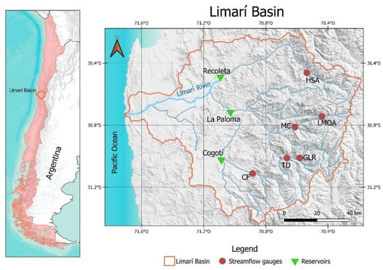
Figure 1.
Map of the Limarí River basin and its location in Chile.
Table 2.
Comparison of observed (obs) and simulated (sim) streamflows for calibration and validation periods.
The current operation rule of the system was developed by Ferrer et al. [93], who used precipitation and streamflow data from 1944 to 1976 to simulate the inter-annual variability and various allocation scenarios. Ferrer et al. [93], estimated volumes of 138 and 220 Mm3 for the 3- and 4-year moving average of the annual inflows to the system with 85% exceedance probability, respectively. The moving average inflows with 85% exceedance probability are important because they give information about the maximum amount of water that can be allocated, while keeping a time-based reliability of 85%, which restricts the maximum amount of water rights that can be allocated in Chile [92]. After analyzing the historical hydrology, Ferrer et al. [93] concluded that a wet year is expected to follow three dry years. Hence, a period of three years was considered critical for the long-term operation of the reservoir system, leading to a single annual allocation decision [93]. Based on this analysis Ferrer et al. [93] determined the operation rule and the amount of water to be allocated from each reservoir that has been operating ever since (Equation (5), depicted at the end of this section).
More formally, the system operation is expressed as follows. The stored volume () in reservoir j at the beginning of year t + 1 is
where I and Sp are the outflow, inflow, and spilled water, respectively (). For this study, and as depicted in Section 3, inflows (I) are obtained from the WEAP hydrological model, which simulates synthetic streamflows using future climate projections. is the net evaporation from the reservoir ():
where e is the evaporation rate () estimated from meteorological data, P is the precipitation (), and A is the surface area (m2) for reservoir j during year t, associated with the current storage elevation, which in turn is also related to the water storage volume. Given that the stored water cannot exceed the maximum storage capacity , the spilled water () from Equation (1) is excess water that the reservoir is not able to store (Equation (4)). Moreover, usable stored water is restricted by the dead storage (), which is the storage under the lowest discharge outlet, and hence cannot be used:
Although the relation between surface area and water stored in the reservoirs may change through time, for simplification we assume the original design for each reservoir (i.e., dead storage, maximum storage and the relationship between the surface area and the stored volume) to remain constant.
The water allocated in year t + 1 () is a function of the stored water in the system composed of M reservoirs at year t (), where is obtained from Equation (1). If overpasses a threshold or restrain bound (RB), a fixed amount is allocated from reservoir j. Otherwise, the allocated water is a fraction r of the storage.
Ferrer et al. [93] determined values of α = 240, 40 and 40 Mm3 for the Paloma, Recoleta, and Cogotí reservoirs, respectively, as well as values of = 500 Mm3 and = 0.5. Thus, if the system storage exceeds 500 Mm3, the maximum allowed annual water allocation is 320 Mm3. Otherwise, half of the stored water is allocated. Note that, although it may be uncommon for other places, the reservoir operation is based on an annual decision, which has been successfully used for more than four decades. As we aim to evaluate when climate change may significantly impair their performance, identifying the timing for adaptation strategies to be implemented, we need to assess the current reservoir operation rule instead of a theoretical or optimized new operation that could be defined at a different time scale (monthly or other). Furthermore, changing water allocation goals might not be simple in Chile, as according to the 1981 Water Code water use rights are legally treated as real state private property, which are granted to perpetuity. Hence, modifications in the Water Code may be needed prior to changes in the allocation.
3. Methodology
Several methods and tools are used in this study to analyze the relation between climate, hydrology, the reservoir system, and its performance. An already developed hydrological climate-driven model implemented in the Water Evaluation and Planning (WEAP) system [94,95] was updated and calibrated using historical monthly runoff data. This model is utilized to generate streamflow scenarios for the operation of the reservoirs’ system using synthetic local climate projections as input. For the generation of these projections, precipitation, and temperature data for the period 1971–2100 from 49 runs of GCMs (Appendix A) and the four RCPs (i.e., 149 climate projections) were downscaled with a weather generator. Finally, the performance of the reservoirs’ system under this set of streamflow scenarios was characterized through performance indexes. Figure 2 depicts the methodology, with a special focus on the implementation of Equations (1)–(5) to simulate the reservoirs’ operation, particularly the water allocation. Details of the methodology are presented in the subsections below.

Figure 2.
Schematic representation of the methodology. The general flow chart is presented in the upper part, and the detail of the reservoir operation are shown in the lower part.
3.1. Hydrological Modeling
WEAP uses climate information as input to generate streamflow following a semi-distributed approach. In the model, elevation bands are used as hydrological units where climate, soil, topography, and land use characteristics are specified. A WEAP model already set up for the Limarí Basin by Vicuña et al. [40,41] was re-calibrated and used in this study. The re-calibration used the most recent years (1985–2011), leaving the period 1969–1984 for validation. Because this approach allows obtaining calibration parameter from a more recent period, the time lag between the periods of calibration and simulation using to future climate projections is reduced, and more reliable hydrologic simulations are obtained [96]. Overall, the simulated and observed hydrographs are similar, and satisfactory Nash–Sutcliffe efficiency (NSE) coefficient values [97] were obtained for the different streamflow gauges (Table 2); furthermore, observed and simulated average annual flows are very similar for the calibration period. The model tends to underestimate the annual flow for the validation period, while the coefficient of variation (CV) is underestimated for the entire historic period mainly due to the underestimation of the extreme discharge values during very humid months. Given that extreme discharges tend to produce water spills in the reservoir operation, the underestimation of them does not affect the performance of the simulation of the operation rule. In the validation period the NSE value improves, compared to the calibration period for the San Agustín and Ojos de Agua gauges, is maintained for Cuestecita gauge and decreases for Las Ramadas, Desembocadura, and Fragüita gauges (Table 2). Flow discharges simulated at the San Agustin gauge are the least satisfactory (Figure 3). This gauge receives contributions from the highest elevations in the basin (>5000 m) where reliable meteorological measurements are scarce. Nonetheless, even at this gauge low flows (i.e., the most relevant flows for the long-term simulation of the basin) are well simulated. Moreover, Table 2 shows good simulations associated with the main tributaries contributing to the system (i.e., Las Ramadas, Fragüita, and Cuestecita). These contributions explain most of the inflows to Cogotí and Paloma reservoirs, which represent 90% of the system storage volume. For a more detailed description of the implemented WEAP model, readers are referred to the references by Vicuña et al. [40,41].
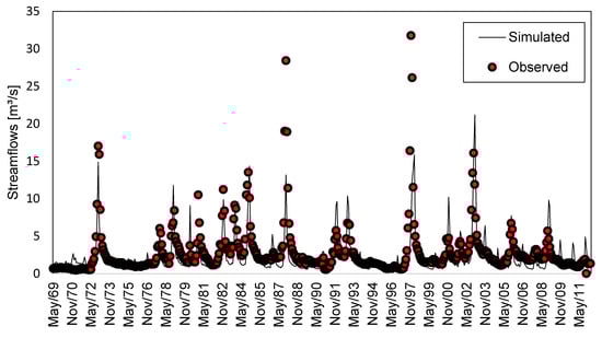
Figure 3.
Observed vs. simulated monthly discharges for the period 1969–2011 at the San Agustin gauge in the Hurtado River.
3.2. Development of Climate Change Scenarios
Under the premise that many GCMs are needed to characterize the uncertainty when analyzing climate change impacts, this study considered 49 GCMs realizations (Appendix A) and the RCPs 2.6, 4.5, 6.0, and 8.5 [98,99]. GCMs’ projected precipitation and temperature series were downscaled using a weather generator downscaling method, obtaining 200 synthetic time series of climates, under each RCP scenario, for the period 1970–2100. In the first step, GCM outputs are interpolated using inverse square distance to the ground weather station locations.
The Chadwick et al. [90] annual weather generator downscaling method was adopted, which considers (1) the extraction of long-term trends from the changes of the mean and the standard deviation from a GCM group, and (2) the generation of annual climate (i.e., precipitation and temperature) time series based on these trends, and the historical observed climate between 1971 and 2005. The trends are extracted from the changes of a GCM group for each RCP. Changes in the precipitation mean from the GCM projection G are obtained by the ratio between the moving averages of the GCM precipitation () and the average from the GCM control period (), where t and are the last year of the moving window and the control period, respectively. This ratio is called normalized moving average . The trends are built using all the from each RCP. For each year t an empirical cumulative distribution function (CDF) of all the is fitted. Finally, the trend percentile with a non-exceedance probability , , is obtained from the CDFs of each year. Note that corresponds to a statistical mapping of the changes from a GCM group, and several trend percentiles can be used to map the dispersion among the group of GCM results.
An analogous process is undertaken for the standard deviation of the precipitation. The trend percentile of the standard deviation () with a non-exceedance probability is randomly generated considering the average correlation with the trend percentile of the mean, which is chosen. For temperature, a similar process for extracting the trends is applied, but the normalized moving difference between moving average of temperature and the average of the control period of the GCM is used instead. Moreover, the non-exceedance probability and for the change of the mean and the standard deviation of the temperature, are also randomly generated considering their average correlation with the trend percentile of .
For the generation of annual climate series data, in each station of interest probability distribution functions (PDFs) are fitted to the observed annual records of the variable Y (temperature or precipitation) through estimation of the parameter set using the mean , and standard deviation . These PDFs are combined with the GCMs trend percentiles, case in which the parameter set change in time according to the GCMs. Hence, this is a GCM ensemble that incorporates the natural variability. Under this approach, the value of the climatic variable at any time for a given and RCP is the value obtained from the PDF, but with mean and standard deviation that change through time according to the trends:
where u is a random uniform number [0,1], and is the annual precipitation value randomly generated, using the trend percentile of the mean, for a non-stationary climate. The value of and in Equation (6) at any particular year t for precipitation are calculated from the historical mean () and standard deviation () and the multiplicative normalized change rates:
For temperature, a similar equation is used, but and are obtained using the additive changes rates, and probabilities and :
Finally, to disaggregate the annual data generated with the weather generator into monthly data, we used the k-Nearest Neighbor (k-NN) method, similar to the one utilized by [100]. Following the heuristic approach adopted elsewhere [101,102], a value of was used in the implementation of the k-NN method, in which is the length of the historical record (i.e., 35 years). For the disaggregation, we have the annual synthetic generated climate for several climate stations (precipitation and temperature) and we also have the historical observed monthly climate at the same stations. To disaggregate one year of the synthetic climate, we sort in ascending order, the historical years of climate, according to the Euclidian distance between the annual data of each historical year and the synthetic year. For this purpose, equal weighting factors were used for each station, given that we previously standardized the synthetic and observed climate data by subtracting the historical mean and dividing by the historical standard deviation. Then a historical year is chosen by using the k-NN method [101], which is then used to disaggregate annual synthetic climate into monthly climate. The process is repeated for each synthetic year to disaggregate the whole synthetic series. Given that the annual value of the historical year and the synthetic year to be disaggregated not necessarily match, there is a post adjustment by multiplication and addition in the case of precipitation and temperature, respectively.
As explained above, using trend percentiles allows mapping the dispersion of the group of GCM runs for each RCP and the local climate information. Ten equally spaced trend percentiles for the changes in the precipitation mean are adopted, as recommended by Chadwick et al. [90], while the trend percentiles of the precipitation standard deviation, temperature mean and standard deviation, are randomly selected considering the correlation among them [90]. For each trend percentile 20 synthetic realizations are generated, adding the total of 200 synthetic realizations for each RCP scenario.
3.3. Performance Indexes
First, satisfactory and unsatisfactory states must be defined to assess the system performance. A satisfactory state is that when the total annual demand () is met, whereas the system falls into an unsatisfactory state or failure when is not satisfied. Hence, the Paloma system is on failure when the long-term expected annual water allocation is under (see Equation (5)). The performance criterion used are the RRV indexes proposed by Hashimoto et al. [27], and widely used in the literature [28,29,31,46,55,103,104,105,106,107,108].
Time-based Reliability () measures how often the system fails. This index is calculated as the percentage of time (0–1 range) that the system can meet in the n years under evaluation:
where counts the number of years at failure:
where equals 1 each time step in which the system passes from failure to success and 0 if it stays on failure. Hence, , which ensures a Res range between 0 (no recovery from failure or always in failure) to 1 (immediate recovery from failure or never in failure).
The Volume-based Reliability () [55,109] was also used in the analysis:
hence, ranges between 0 and 1 and measures the mean percentage of water allocated by the system compared to .
Following the approach by [106,107], two indexes for vulnerability were used: (1) the maximum vulnerability or maximum water deficit () as used by Moy et al. [32], and (2) the average vulnerability or average water deficit (. Both indexes range between 0 and 1, and are
where
In Equations (14) and (16), vulnerability values are standardized by .
4. Results and Analysis
4.1. Climate Change Hydrological Impacts
Future annual precipitation and reservoir inflow projections are presented in Figure 4 and Figure 5 for the la Paloma reservoir. Both figures show the 25th, 50th, and 75th percentiles of the time series averaged over a 40-year moving window. Precipitation starts with 117 mm (50th percentile) by year 2010 (Figure 4) and decline in time to 107 mm, 99 mm, 97 mm, and 88 mm, by the end of the century under RCPs 2.6, 4.5, 6.0, and 8.5, respectively; these changes correspond to reductions of −8.5%, −15.4%, −17.1%, and −24.7%, respectively. Furthermore, larger declines are observed for higher percentiles, regardless the RCP; for example, under RCP 2.6 reductions of 9, 10, and 19 mm are obtained for the 25th, 50th, and 75th percentiles, respectively. Hence the climate is projected to become drier, with larger precipitation reductions for the rainy years.

Figure 4.
Projected precipitation for the Paloma Embalse station gauge (320 m a.s.l., 30°41′48″ S, 71°02′18″ W) under RCP 2.6 (a), 4.5 (b), 6.0 (c) and 8.5 (d). The 25th (dotted line), 50th (solid line), 75th (dashed line) of annual percentiles is averaged over a 40-year moving window, with the horizontal axis being the last year of the window.
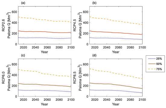
Figure 5.
Projected inflow to the Paloma reservoir under RCP 2.6 (a), 4.5 (b), 6.0 (c), and 8.5 (d). The 25th (dotted line), 50th (solid line), 75th (dashed line) of annual inflows to the Paloma reservoir are averaged over a 40-year moving window, with the horizontal axis being the last year of the window.
The impacts of these precipitation changes over the incoming streamflow to the Paloma reservoir is magnified (Figure 5). The 50th percentile of the inflow goes from 245 Mm3 by 2010, to 218, 179, 179, and 147 Mm3 by 2100 under RCPs 2.6, 4.5, 6.0, and 8.5, respectively; these changes correspond to reductions of −11.4%, −27.2%, −25.1%, and −40.7%, respectively. Just as for precipitation, the absolute decline is greater for higher percentiles. For example, under RCP 2.6 the inflows to the Paloma are projected to diminish in 9, 28 and 82 Mm3 for the 25th, 50th, and 75th percentile between years 2010 and 2100.
Similarly, inflows to the Cogotí and Recoleta reduce through time, as shown in Figures S1 and S2 in the Supplementary Material. Nonetheless, these reductions are even larger, most likely because the contributing areas to these reservoirs are located at higher elevation. Starting with a 50th percentile value of 95 Mm3 in 2010, inflows to the Cogotí reservoir decrease to 73, 60, 60, and 48 Mm3 by 2100, under RCPs 2.6, 4.5, 6.0, and 8.5 respectively (Figure S1). These are reductions of −23.2%, −36.8%, −35.5%, and −49.5%, respectively. Likewise, 50th percentiles inflows to the Recoleta reservoir reduce form 60 Mm3 in 2010 to 35, 17, 17, and 12 Mm3 by 2100, under RCPs 2.6, 4.5, 6.0, and 8.5, respectively. These are reductions of −58.3%, −71.2%, −71.2%, and −80.0%, respectively.
Overall, the basin is expected to have a drier future, as concluded by previous studies in the basin [40,41,90]. Interestingly, projected reductions in reservoirs inflow surpass those expected for precipitation, especially in the upper basin. Moreover, reductions in precipitation and streamflow are greater for higher percentiles, which implies fewer very humid years in the future. This decline is quite relevant because the reservoirs are filled precisely during these very humid years.
4.2. Long-Term Impacts over Reservoir Operation
Changes in the RRV performance are analyzed using a 40-year moving window during the 1971–2100 period. The objective is to show in a simple, yet comprehensive manner, how and when future reservoir performance is expected to considerably worsen, and the corresponding uncertainty around this estimation. Thus, the performance associated with any particular year considers the last 40 years of operation. The dynamics of the positive performance metrics (i.e., , and ) are shown in Figure 6, Figure 7 and Figure 8, whereas that of the negative performance metrics (i.e., and ) are shown in Figure 9 and Figure 10. To illustrate the use of thresholds to identify the time at which sever impacts in the system’s operation occur, we adopted in these figures two referential values that are intuitive and easy to follow in decision-making. The first threshold corresponds to the historical reference RRV performance calculated from the first 40 years of operation between 1971 and 2010 (thick dashed lines). The second threshold indicates a 10% worsening of the reference historical RRV performance (thick dotted line). Note however that any threshold value may be used, which can reflect for example a decision by the regulator or operator, a local regulation, or a hypothetical scenario. Following the recommendations from McMillan et al. [87] the uncertainty through time associated with the variety of GCMs is presented in each figure using the 25th, 50th, and 75th percentiles of the corresponding performance indexes (thin dotted, solid, and dashed lines, respectively). To analyze the potential errors of using just 200 synthetic time series per RCP, a bootstrapping analysis was performed as explained in Text S1. The results of the bootstrapping analysis are presented in Figures S3–S12 in the Supplementary Material. Note that the possible errors that may be produced by using only 200 synthetic time series per RCP are quite small (Figures S3–S12).

Figure 6.
Time-based reliability under RCP 2.6 (a), 4.5 (b), 6.0 (c), and 8.5 (d) for a 40-year moving window, with the horizontal axis being the last year of the window. The thick dashed and dotted lines represent the reference historical performance and 10% worse-than-the-reference value, respectively.

Figure 7.
Resilience under RCP 2.6 (a), 4.5 (b), 6.0 (c), and 8.5 (d) for a 40-year moving window, with the horizontal axis being the last year of the window. The thick dashed and dotted lines represent the reference historical performance and 10% worse-than-the-reference value, respectively.

Figure 8.
Volume-based reliability under RCP 2.6 (a), 4.5 (b), 6.0 (c), and 8.5 (d) for a 40-year moving window, with the horizontal axis being the last year of the window. The thick dashed and dotted lines represent the reference historical performance and 10% worse-than-the-reference value, respectively.

Figure 9.
Maximum vulnerability under RCP 2.6 (a), 4.5 (b), 6.0 (c), and 8.5 (d) for a 40-year moving window, with the horizontal axis being the last year of the window. The thick dashed and dotted lines represent the reference historical performance and 10% worse-than-the-reference value, respectively.

Figure 10.
Average vulnerability under RCP 2.6 (a), 4.5 (b), 6.0 (c), and 8.5 (d) for a 40-year moving window, with the horizontal axis being the last year of the window. The thick dashed and dotted lines represent the reference historical performance and 10% worse-than-the-reference value, respectively.
4.2.1. Positive Performance Metrics
According to Figure 6, and regardless the RCP considered, time-based reliability worsens through time, with values being lower than the historical reference value of 0.81, a value that is relatively close to the 0.85 considered in the Chilean regulation as the objective time-based reliability [92]. Nonetheless, time-based reliability varies considerably for the different RCPs, with values around 0.53, 0.45, 0.45, and 0.38 estimated under RCPs 2.6, 4.5, 6.0 and 8.5, respectively, for the 50th GCM percentile by the end of the century. Under RCP 2.6 the interquartile range (i.e., between the 25th and 75th percentile) in 2011 (0.14 between 0.75 and 0.89) doubles by year 2100 (0.29 between 0.39 and 0.68). Under RCP 4.5, the values for the same percentiles go from 0.75–0.88 (i.e., range of 0.13) in 2011 to 0.29–0.60 (i.e., range of 0.31) in 2100. For the RCP 6.0, the values for the percentiles 25th and 75th go from 0.73–0.88 (i.e., range of 0.15) in 2011 to 0.28–0.63 (i.e., range of 0.35) in 2100. Under RCP 8.5, the values for the same percentiles go from 0.73–0.88 (i.e., range of 0.15) in 2011 to 0.20–0.58 (i.e., range of 0.38) in 2100. Overall, the uncertainty of the time-based reliability due to the different GCM increases with time and RCP.
The resilience index for the future period under the four RCPs shows a negative trend with values below the historical resilience of 0.45 (Figure 7). As expected, the future resilience is the best for RCP 2.6 and decreases for the other RCPs. The resilience values for the 50th percentile by 2100 are 0.25, 0.22, 0.22, and 0.19, under RCPs 2.6, 4.5, 6.0, and 8.5, respectively. Thus, the probability of recovering from a failure under RCP 4.5 or higher will be less than half of what it used to be in 2011. Interestingly, the interquartile range of resilience values predicted by the end of the century is smaller than that in 2011, regardless the RCP.
Just as for the other indexes, the volume-based reliability significantly changes under different RCP scenario (Figure 8). The 50th percentile of this index under RCP 2.6 reaches a value of 0.84 by the end of the century, whereas the 25th percentile reaches a value of 0.75 (Figure 8a). Thus, the future performance does not significantly worsen under the lowest emission scenario, compared to the historical reference value of 0.92. The 50th percentile of the volume-based reliability by 2100 are 0.78, 0.78, and 0.73, under the RCPs 4.5, 6.0, and 8.5, respectively. As in the case of the time-based reliability (Figure 6), the uncertainty of the volume-based reliability increases with time and with the RCPs. The values of the 25th and 75th percentiles of this metric for the year 2100 are 0.75–0.91 for RCP 2.6, (Figure 7a), which significantly decrease if higher RCP scenarios are considered: 0.67–0.89 (RCP 4.5, Figure 7b), 0.67–0.88 (RCP 6.0, Figure 8c), and 0.57–0.86 (RCP 8.5, Figure 8d). Thus, the interquartile ranges for year 2100 are 0.16, 0.22, 0.21, and 0.29, under the RCPs 2.6, 4.5, 6.0, and 8.5, respectively.
Given that reductions for the 75th percentile of both precipitation and inflows to the reservoirs are larger than for the 25th percentile (Figure 4 and Figure 5, Figures S1 and S2), the interquartile range for these variables reduces throughout the century. Nevertheless, the interquartile range for both the time-based and volume-based reliabilities increases (Figure 6 and Figure 8). This interesting result illustrate the importance of using reservoir performance indexes to understand the impacts of climate change, as the changes and uncertainties in the raw hydro-climatological variables are not necessarily the same, or transferable, as those for the operational variables defining the performance of water systems in general, and reservoirs in particular.
4.2.2. Negative Performance Metrics
According to Figure 9, the maximum vulnerability increases under the RCP 2.6 scenario, beyond the historical reference value of 0.68, but without surpassing the “Reference + 0.1” threshold (thick dotted black line, Figure 9a). For the other RCPs, the maximum vulnerability worsens in the future beyond this threshold. Nevertheless, this severity has not been an issue yet, as reservoir design in Chile relays mostly on ensuring the time-based reliability. The future maximum vulnerability reaches values larger than 0.80 for the 50th percentile under RCPs 4.5, 6.0, and 8.5, which indicates that severe droughts are projected during the following decades. While a worse future is clearly predicted in terms of the maximum vulnerability index (Figure 9), the average vulnerability behaves differently (Figure 10). Under the four RCPs, the average vulnerability clearly improves by mid-century (2060), with a reduction for the 50th percentile from 0.45 (historical reference), to 0.36, 0.37, 0.38, and 0.36 by year 2060 for RCPs 2.6, 4.5, 6.0, and 8.5, respectively. By the end of the century, the average vulnerability continues improving for RCP 2.6, while for RCPs 4.5 and 6.0 it slightly worsens, although not beyond the reference value of 0.45. For RCP 8.5, the 50th percentile average vulnerability by the end of the century equals the reference value. It is noteworthy that, although the number of failures will likely increase in time (Figure 6), the severities of these failures are expected to reduce by the middle of the century (Figure 10). Most likely the average vulnerability improves because the time-based reliability (Figure 6) worsens more than the volume-base reliability (Figure 8), hence the failures become more recurrent, but less severe. Nevertheless, the maximum failure increases (Figure 9), so even if the average failure (Figure 10) is not as bad, the worst drought is expected to be worse. Note, that all these results depend on the reservoir operation rule; thus, if the current reservoir operation rule is modified, the expected consequences will need to be re-evaluated.
4.3. The Timing of the Changes in Performance: When Current Management Will Become Obsolete?
To identify the time when the current reservoir operation rule is no longer able to maintain the historical reference performance (i.e., time of emergence, ToE), we compute the first year in which the 50th percentile of each performance index exceeds a 10% worse-than-the-reference value, without going back (Table 3). Table 3 also shows in parenthesis the 80% confidence range for the 50th percentile emergence (i.e., 10% and 90% of error), estimated with the bootstrapping (Figures S3–S12 in the Supplementary Material). Under RCP 2.6 the ToE for the time-based reliability and resilience indexes is identified within the century, while for the other indexes it is not. Moreover, the ToE for the average vulnerability does not take place in this century for any of the four RCPs. Under RCPs 4.5 and above, the ToE detected for each index are clearly different: the time-based reliability overpasses the threshold between years 2028 and 2033, the resilience diverges from the reference between 2034 and 2042, whereas the volume-based reliability does so between 2072 and 2083, and the maximum vulnerability index overpass the reference threshold between 2068 and 2079. Overall, under RCPs 4.5 and above, Table 3 shows that the 10% worse-than-the-reference value is exceeded during the 2030s in terms of the time-based reliability, the 2030s and 2040s in terms of the resilience, the 2080s in terms of volume-based reliability, and the 2070s in terms of maximum vulnerability.
Table 3.
First year in which, for each RCP and performance index, the 50th percentile reservoir performance exceeds a 10% worse-than-the-reference value without going back. In parenthesis are the same result, but for the 10% and 90% of error estimated with the bootstrapping (Supplementary Material).
If the 25th and 75th percentiles are used instead the 50th percentile to analyze the ToE, we can appreciate the uncertainty associated with the results. For example, the time-based reliability under RCP 2.6, overpass the threshold on years 2016 and 2067 for the 25th and 75th percentile (Figure 6a), respectively. Under RCP 8.5 the years are now 2013 and 2057 for the same percentiles (Figure 6d). For the volume-based reliability (Figure 8) under RCP 8.5, the ToE for the 25th percentile is year 2047, but for the 75th percentile it happens after 2100. The maximum vulnerability threshold for the 25th percentile (Figure 9) is not overpassed by any RCP during this century. Overall, the large time range detected when using the 25th and 75th percentile illustrates how difficult it is to identify a single year in which the reservoir performance will stop performing as expected historically, rather only a range of many years can be identified. This issue is further discussed by Chadwick et al. [83].
A comparison of the values in Table 3 against the 50th percentile Local ToE estimates for precipitation and temperature in the same basin [83] shows that deviations from the historical behavior of the reservoir performance, measured using time-based reliability or resilience, occur slightly before than for precipitation. On contrary, ToE takes place after when considering other performance indexes. For example, the time-based reliability performance for the 50th percentile (Figure 6) worsens before 2040 for RCPs 4.5 and 8.5, while changes in precipitation in the basin happen around 2040 [83]. Such difference is likely caused in part by the early emergence of changes in temperature. Interestingly, the ToE for the volume-based reliability under RCP 4.5 and above (Figure 8) happens during the 2080s for the 50th percentile, while changes in precipitation emerge earlier [83]. Nevertheless, further analysis is needed, given the larger uncertainty in the timing of changes in reservoir performance, as there are more steps involved in the cascade of uncertainty associated with the calculations [42]. Moreover, the results from our analysis allows detecting ToE that differ among the different performance indexes. In our case for example, time-based reliability (Figure 6) is affected before the volume-based one (Figure 8), and thus adaptation measurements should be taken before the occurrence of significant changes in volume-based water allocation.
Overall, our approach and results are presented as a replicable method to inform decision makers—in a clear, simple, and useful manner—about the impacts of climate change through time over the performance of a reservoir operation rule. In particular, by defining an easy-to-follow and intuitive percentage worse-than-the-reference value to evaluate the performance, one can identify the time of obsolescence of the current operation rule under a climate change scenario (i.e., a local ToE of the reservoir performance). Furthermore, our approach allows transmitting the uncertainty to water managers and practitioners using uncertainty bands or alike, something recommended in the literature in recent years [87].
4.4. Adaptation Strategies
Although the main objective of this article is to depict an approach to identify the time at which the performance will drop beyond a defined threshold due to climate change under the current operation rule (i.e., ToE of reservoir performance), we now explore in a simple manner the implications of possible adaptations strategies. It is not our goal to optimize the operation rule, but to illustrate how the approach allows understanding the effect of varying the operation rule (i.e., reduction of water allocation goals) to cope with the increasing water scarcity of the basin. Given that the most severe changes and earlier emergences are expected under RCP 8.5, we use this scenario for the analysis. In particular, we explore the effects of implementing different reductions in water allocation goals in year 2033, when the first emergence is detected for this RCP. For example, Figure 11 compares the performance indexes obtained when the water allocation goals are reduced to 205, 35, and 35 Mm3, for the Paloma, Cogotí, and Recoleta reservoirs, respectively (green lines), against the reference case in which the operation rule remains the same (red lines). For this case, the impacts of the change in the rule differ depending on the index. Resilience is barely affected, while both vulnerability metrics are reduced to the point that the 50th percentile MaxV and AvgV remain respectively within the ±0.1 reference and the reference thresholds by 2100.

Figure 11.
Performance indexes obtained using the current operation rule (red) and a reduced allocation goal implemented the ToE year (2033) as an adaptation strategy (green). The adaptation (current) allocation goal is 205 (240), 35 (40), and 35 (40) Mm3, for the Paloma, Cogotí, and Recoleta reservoirs, respectively. Indexes include the time-based reliability (a), resilience (b), volume-based reliability (c), maximum vulnerability (d) and average vulnerability (e), for a 40-year moving window, with the horizontal axis being the last year of the window. The thick dashed and dotted lines represent the reference historical performance and 10% worse-than-the-reference value, respectively.
Similar results to those shown in Figure 11 can be calculated for other reductions in the allocation goals (not shown here). To summarize these results, Table 4 presents the first year in which the 50th percentile reservoir performance indexes values exceed a 10% worse-than-the-reference value without going back, under RCP 8.5, for different adaptation strategies (i.e., reductions in annual water allocation goals) as shown in columns 1–4. As expected, for each index the year in which the threshold is exceeded delays with larger reductions in water allocation goals. Nevertheless, in order for the system to perform as originally expected throughout the 21st century, reductions of 40–50% of the original system allocation goal are needed. Such reductions may be extremally difficult to implement in the basin, and thus the eventual adaptation process may require the strong involvement of stakeholders and the compromising of current expectations.
Table 4.
First year in which, for different allocation goal reductions, the 50th percentile reservoir performance exceeds a 10% worse-than-the-reference value with no turning back under RCP 8.5. Columns 1 and 2 show annual allocation goals for each reservoir, and columns 3 and 4 show the corresponding system allocation goal as volume and as a percentage of the original 320 Mm3.
5. Conclusions
This study assessed the operation of a reservoir system using the RRV performance indexes during the 21st century under climate change. Considering the ongoing water scientist’ challenge of communicating climate change results in a usable way for water managers, the results focus on providing a clear response to the decision-making question: when current operation rules will significantly impair their performance due to climate change impacts?
For this purpose, the future performance of the Paloma reservoir system in the Limarí River basin, Chile, was evaluated using a 40-year moving window for the period 1971–2100. Using a weather generator, GCMs outcomes were downscaled to produce climate series that served as input to an already set up WEAP hydrological model, which was utilized to simulate streamflows. These flows were used to model the performance of the historical and future operation of the reservoir system under the current operation rule, which was characterized using percentiles of the RRV indexes. For illustrative purposes, this performance was defined to be deficient when the RRV indexes worsen more than a 10% as compared to the historical values; however, any other threshold can be selected by the operator or the decision maker. The approach adopted in this study allows estimating the impacts of climate change while accounting for three sources of uncertainty: (a) aleatory uncertainty, i.e., the natural variability represented by intra-GCM uncertainties, (b) epistemic uncertainty, i.e., as represented by the spread of multi-GCM ensembles, and (c) deep uncertainty, i.e., as represented by the choice of RCP scenario. Note that the methodology here presented treats aleatory and epistemic uncertainties in a risk analysis, while deep uncertainty is properly presented. Thus, we aimed to clearly disentangle and communicate the impacts of climate change from the very considerable noise of these three sources of uncertainty. Our main conclusions are the following:
- -
- Precipitation reductions are projected in the basin due to climate change. While inflows to the reservoirs are also projected to diminish, there is an amplified response of streamflows, which will reduce even more than precipitation, especially in the upper basin.
- -
- The time-based reliability of the Paloma system will deteriorate significantly in the future, even for an optimistic percentile (75th), under all the RCP scenarios. The volume-based reliability will also reduce, except for the RCP 2.6 scenario. Thus, mitigation measures become key to ensure an adequate reservoir system’s performance during the next decades.
- -
- Counterintuitively, although the projected time-based and volume-based reliability worsen in time, the average vulnerability stays around the historical value by the end of the century. In fact, the average vulnerability improves by mid-century (2060) regardless the RCP scenario, and tends to go back to the reference for RCPs 4.5 and above.
- -
- The range of GCMs uncertainty increases for the time-based and volume-based reliability, both with time and RCP scenario (i.e., RCP uncertainty decreases from RCP 8.5 to RCP 2.6). On the other hand, this range decreases with time for precipitation and reservoir inflows, while staying quite constant with the RCP.
- -
- The emergence was detected much earlier for the time-based reliability than for the volume-based one. Hence a new operation rule will be needed earlier if the time-based reliability is considered as the predominant performance metric. Indeed, this is the case in Chile, and thus the current operation rule should be changed in the 2030s. Nevertheless, the best timing to change the operation rule still depends on the RCP scenario, as well as the performance threshold, which should be discussed and defined by decision makers.
- -
- Deviations from the historical behavior of the reservoir performance measured using time-based reliability or resilience, occur slightly before than precipitation changes. On contrary, these deviations take place after when considering other performance indexes (i.e., volume-based reliability and maximum vulnerability). Hence, the identification of the ToE of variables other than the climatic ones (i.e., precipitation and temperature) that are more directly related to water resources availability becomes relevant. Nonetheless, such identification is more uncertain as more steps in the cascade of uncertainty are involved.
- -
- For the Paloma system to perform as originally expected throughout the 21st century, reductions of 40–50% of the original system allocation goal are needed under RCP 8.5. Given the difficulty of implementing such reductions in the basin, any eventual adaptation process will require the strong involvement of stakeholders and the compromising of current expectations.
We believe the approach followed in this study allows decision maker to easily understand climate change risks and impacts, and to identify the critical timing to propose and implement adaptation measures affecting current operation rules, infrastructure, and water allocation goals, especially in cases were implementing those changes are difficult or timely to implement. Although this work does not explore adaptation alternatives, their performance through time, as well as their prioritization, can also be assessed within this framework. On the other hand, in a direct and relevant application, this work can be extended nationwide, allowing the prioritization of resources where adaptation is or will be needed sooner. Finally, future studies considering other downscaling methods and different hydrological modeling approaches should be carried out to quantify their effects on the reservoir’s performance assessment. Moreover, other dynamics in the basin and the reservoirs’ system may be incorporated, such as land-uses changes and changes in the reservoirs capacity and dead storages due to sedimentation [110,111].
Supplementary Materials
The following are available online at https://www.mdpi.com/2073-4441/13/1/64/s1, Figure S1: Projected inflow to the Cogotí reservoir under RCP 2.6 (a), 4.5 (b), 6.0 (c), and 8.5 (d). The 25th (dotted line), 50th (solid line), 75th (dashed line) of annual inflows to the Cogotí reservoir are averaged over a 40-year moving window, with the horizontal axis being the last year of the window; Figure S2: Projected inflow to the Recoleta reservoir under RCP 2.6 (a), 4.5 (b), 6.0 (c), and 8.5 (d). The 25th (dotted line), 50th (solid line), 75th (dashed line) of annual inflows to the Recoleta reservoir are averaged over a 40-year moving window, with the horizontal axis being the last year of the window; Text S1: Bootstrapping Method; Figure S3: Time-based reliability under RCP 2.6 (a), 4.5 (b), 6.0 (c), and 8.5 (d) for a 40-year moving window, with the horizontal axis being the last year of the window. The thick dashed and dotted lines represent the reference historical performance and 10% worse-than-the-reference value, respectively. The red lines are the same results from Figure 5a,b, with the thin blue and yellow lines being the 10% and 90% of error, obtained with the bootstrapping method explained in Text S1; Figure S4: Time-based reliability under RCP 2.6 (a), 4.5 (b), 6.0 (c), and 8.5 (d) for a 40-year moving window, with the horizontal axis being the last year of the window. The thick dashed and dotted lines represent the reference historical performance and 10% worse-than-the-reference value, respectively. The red lines are the same results from Figure 5c,d, with the thin blue and yellow lines being the 10% and 90% of error, obtained with the bootstrapping method explained in Text S1; Figure S5: Resilience under RCP 2.6 (a), 4.5 (b), 6.0 (c), and 8.5 (d) for a 40-year moving window, with the horizontal axis being the last year of the window. The thick dashed and dotted lines represent the reference historical performance and 10% worse-than-the-reference value, respectively. The red lines are the same results from Figure 6a,b, with the thin blue and yellow lines being the 10% and 90% of error, obtained with the bootstrapping method explained in Text S1; Figure S6: Resilience under RCP 2.6 (a), 4.5 (b), 6.0 (c), and 8.5 (d) for a 40-year moving window, with the horizontal axis being the last year of the window. The thick dashed and dotted lines represent the reference historical performance and 10% worse-than-the-reference value, respectively. The red lines are the same results from Figure 6c,d, with the thin blue and yellow lines being the 10% and 90% of error, obtained with the bootstrapping method explained in Text S1; Figure S7: Volume-based reliability under RCP 2.6 (a), 4.5 (b), 6.0 (c), and 8.5 (d) for a 40-year moving window, with the horizontal axis being the last year of the window. The thick dashed and dotted lines represent the reference historical performance and 10% worse-than-the-reference value, respectively. The red lines are the same results from Figure 7a,b, with the thin blue and yellow lines being the 10% and 90% of error, obtained with the bootstrapping method explained in Text S1; Volume-based reliability under RCP 2.6 (a), 4.5 (b), 6.0 (c), and 8.5 (d) for a 40-year moving window, with the horizontal axis being the last year of the window. The thick dashed and dotted lines represent the reference historical performance and 10% worse-than-the-reference value, respectively. The red lines are the same results from Figure 7c,d, with the thin blue and yellow lines being the 10% and 90% of error, obtained with the bootstrapping method explained in Text S1; Figure S9: Maximum vulnerability under RCP 2.6 (a), 4.5 (b), 6.0 (c), and 8.5 (d) for a 40-year moving window, with the horizontal axis being the last year of the window. The thick dashed and dotted lines represent the reference historical performance and 10% worse-than-the-reference value, respectively. The red lines are the same results from Figure 8a,b, with the thin blue and yellow lines being the 10% and 90% of error, obtained with the bootstrapping method explained in Text S1; Figure S10: Maximum vulnerability under RCP 2.6 (a), 4.5 (b), 6.0 (c), and 8.5 (d) for a 40-year moving window, with the horizontal axis being the last year of the window. The thick dashed and dotted lines represent the reference historical performance and 10% worse-than-the-reference value, respectively. The red lines are the same results from Figure 8a,b, with the thin blue and yellow lines being the 10% and 90% of error, obtained with the bootstrapping method explained in Text S1; Figure S11: Average vulnerability under RCP 2.6 (a), 4.5 (b), 6.0 (c), and 8.5 (d) for a 40-year moving window, with the horizontal axis being the last year of the window. The thick dashed and dotted lines represent the reference historical performance and 10% worse-than-the-reference value, respectively. The red lines are the same results from Figure 9a,b, with the thin blue and yellow lines being the 10% and 90% of error, obtained with the bootstrapping method explained in Text S1; Figure S12: Average vulnerability under RCP 2.6 (a), 4.5 (b), 6.0 (c), and 8.5 (d) for a 40-year moving window, with the horizontal axis being the last year of the window. The thick dashed and dotted lines represent the reference historical performance and 10% worse-than-the-reference value, respectively. The red lines are the same results from Figure 9c,d, with the thin blue and yellow lines being the 10% and 90% of error, obtained with the bootstrapping method explained in Text S1.
Author Contributions
All authors contributed extensively to the work here presented. S.V. contributed with the hydrological modelling. F.M. and C.C. conceptualized the experiment. C.C., J.G., and P.B. contributed to data analysis. C.C., P.B., S.V. and J.G. contributed to literature review. C.C. and P.B. prepared the original draft. C.C., P.B., J.G., F.M., and S.V. reviewed and edited the manuscript. All authors have read and agreed to the published version of the manuscript.
Funding
This research received funding from research projects Fondecyt 1200135, International Development Research Center Grant 107081-001, the Vicerrectoría de Investigación y Desarrollo (VID) from Universidad de Chile (grant UI-007/19), and grants CONICYT/FONDAP/15110017 and 15110020. Also, funding from the scholarships from CONICYT (21160861), Canada-Chile Leadership Exchange program, Sociedad de Canal del Maipo and the VRI at Universidad Católica were received by Cristián Chadwick.
Institutional Review Board Statement
Not applicable.
Informed Consent Statement
Not applicable.
Data Availability Statement
Publicly available datasets were used in this study. This data can be found here: DGA meteorological data [http://snia.dga.cl/BNAConsultas/reportes], and CMIP5 climatic data [https://esgf-node.llnl.gov/projects/cmip5/].
Acknowledgments
We thank the World Climate Research Programme’s Working Group on Coupled Modelling and the climate modeling groups for making available their models. Meteorological data were obtained from DGA, Chile (http://snia.dga.cl/BNAConsultas/reportes). We also thank Álvaro Zambrano for helping us in the preparation of some figures. We finally thank the referees for their constructive suggestions.
Conflicts of Interest
The authors declare no conflict of interest.
Appendix A
Table A1.
General Circulation Models (GCM) and RCP scenarios used in this study.
Table A1.
General Circulation Models (GCM) and RCP scenarios used in this study.
| GCM Name | Realization | RCP 2.6 | RCP 4.5 | RCP 6.0 | RCP 8.5 | |
|---|---|---|---|---|---|---|
| 1 | ACCESS1.0 | r1i1p1 | x | x | ||
| 2 | BCC-CSM1.1 | r1i1p1 | x | x | x | x |
| 3 | CanESM2 | r1i1p1 | x | x | x | |
| 4 | CanESM2 | r2i1p1 | x | x | x | |
| 5 | CanESM2 | r3i1p1 | x | x | x | |
| 6 | CanESM2 | r4i1p1 | x | x | x | |
| 7 | CanESM2 | r5i1p1 | x | x | x | |
| 8 | CCSM4 | r1i1p1 | x | x | x | x |
| 9 | CCSM4 | r2i1p1 | x | x | x | x |
| 10 | CCSM4 | r3i1p1 | x | x | x | x |
| 11 | CCSM4 | r4i1p1 | x | x | x | x |
| 12 | CCSM4 | r5i1p1 | x | x | x | x |
| 13 | CNRM-CM5 | r10i1p1 | x | |||
| 14 | CNRM-CM5 | r1i1p1 | x | x | ||
| 15 | CNRM-CM5 | r2i1p1 | x | |||
| 16 | CNRM-CM5 | r4i1p1 | x | |||
| 17 | CNRM-CM5 | r6i1p1 | x | |||
| 18 | CSIRO-Mk3.6.0 | r10i1p1 | x | x | x | x |
| 19 | CSIRO-Mk3.6.0 | r1i1p1 | x | x | x | x |
| 20 | CSIRO-Mk3.6.0 | r2i1p1 | x | x | x | x |
| 21 | CSIRO-Mk3.6.0 | r3i1p1 | x | x | x | x |
| 22 | CSIRO-Mk3.6.0 | r4i1p1 | x | x | x | x |
| 23 | CSIRO-Mk3.6.0 | r5i1p1 | x | x | x | |
| 24 | CSIRO-Mk3.6.0 | r6i1p1 | x | x | x | x |
| 25 | CSIRO-Mk3.6.0 | r7i1p1 | x | x | x | x |
| 26 | CSIRO-Mk3.6.0 | r8i1p1 | x | x | x | x |
| 27 | CSIRO-Mk3.6.0 | r9i1p1 | x | x | x | x |
| 28 | FGOALS-g2 | r1i1p1 | x | x | x | |
| 29 | GFDL-CM3 | r1i1p1 | x | x | x | x |
| 30 | GFDL-ESM2G | r1i1p1 | x | x | x | x |
| 31 | GFDL-ESM2M | r1i1p1 | x | x | x | x |
| 32 | GISS-E2-R | r1i1p1 | x | x | x | x |
| 33 | GISS-E2-R | r2i1p1 | x | |||
| 34 | GISS-E2-R | r3i1p1 | x | |||
| 35 | GISS-E2-R | r4i1p1 | x | |||
| 36 | GISS-E2-R | r5i1p1 | x | |||
| 37 | INM-CM4 | r1i1p1 | x | x | ||
| 38 | IPSL-CM5A-LR | r1i1p1 | x | x | x | |
| 39 | IPSL-CM5A-LR | r2i1p1 | x | x | ||
| 40 | IPSL-CM5A-LR | r3i1p1 | x | x | ||
| 41 | IPSL-CM5A-MR | r1i1p1 | x | x | x | |
| 42 | MIROC5 | r1i1p1 | x | x | x | x |
| 43 | MIROC-ESM | r1i1p1 | x | x | x | x |
| 44 | MIROC-ESM-CHEM | r1i1p1 | x | x | x | x |
| 45 | MPI-ESM-LR | r1i1p1 | x | x | x | |
| 46 | MPI-ESM-LR | r2i1p1 | x | x | x | |
| 47 | MPI-ESM-LR | r3i1p1 | x | x | x | |
| 48 | MRI-CGCM3 | r1i1p1 | x | x | x | |
| 49 | NorESM1-M | r1i1p1 | x | x | x | x |
References
- Water for Sustainable Food and Agriculture. A Report Produced for the G20 Presidency of Germany; Food and Agriculture Organization: Rome, Italy, 2017. [Google Scholar]
- Stocker, T.F.; Qin, D.; Plattner, G.K.; Tignor, M.M.B.; Allen, S.K.; Boschung, J.; Nauels, A.; Xia, Y.; Bex, V.; Midgley, P.M. Climate Change 2013: The Physical Science Basis. Intergovernmental Panel on Climate Change, Working Group I Contribution to the IPCC Fifth Assessment Report (AR5); Cambridge University Press: New York, NY, USA, 2013. [Google Scholar]
- Lemos, M.C.; Kirchhoff, C.J.; Ramprasad, V. Narrowing the climate information usability gap. Nat. Clim. Chang. 2012, 2, 789. [Google Scholar] [CrossRef]
- Van Wyk, E.; Roux, D.J.; Drackner, M.; McCool, S.F. The impact of scientific information on ecosystem management: Making sense of the contextual gap between information providers and decision makers. Environ. Manag. 2008, 41, 779–791. [Google Scholar] [CrossRef] [PubMed]
- Ziervogel, G.; Johnston, P.; Matthew, M.; Mukheibir, P. Using climate information for supporting climate change adaptation in water resource management in South Africa. Clim. Chang. 2010, 103, 537–554. [Google Scholar] [CrossRef]
- Field, C.B.; Barros, V.R.; Mastrandrea, M.D.; Mach, K.J.; Abdrabo, M.A.K.; Adger, N.; Anokhin, Y.A.; Anisimov, O.A.; Arent, D.J.; Barnett, J.; et al. Summary for Policymakers. In Climate Change 2014: Impacts, Adaptation, and Vulnerability. Part A: Global and Sectoral Aspects. Contribution of Working Group II to the Fifth Assessment Report of the Intergovernmental Panel on Climate Change; Cambridge University Press: New York, NY, USA, 2014; pp. 1–32. [Google Scholar]
- Paton, F.L.; Maier, H.R.; Dandy, G.C. Relative magnitudes of sources of uncertainty in assessing climate change impacts on water supply security for the Southern Adelaide water supply system. Water Resour. Res. 2013, 49, 1643–1667. [Google Scholar] [CrossRef]
- Risbey, J.S. Dangerous climate change and water resources in Australia. Reg. Environ. Chang. 2011, 11, 197–203. [Google Scholar] [CrossRef]
- Ahmad, A.; El-Shafie, A.; Razali, S.F.M.; Mohamad, Z.S. Reservoir optimization in water resources: A review. Water Resour. Manag. 2014, 28, 3391–3405. [Google Scholar] [CrossRef]
- Beh, E.H.Y.; Maier, H.R.; Dandy, G.C. Adaptive, multiobjective optimal sequencing approach for urban water supply augmentation under deep uncertainty. Water Resour. Res. 2015, 51, 1529–1551. [Google Scholar] [CrossRef]
- Beh, E.H.Y.; Maier, H.R.; Dandy, G.C. Scenario driven optimal sequencing under deep uncertainty. Environ. Model. Softw. 2015, 68, 181–195. [Google Scholar] [CrossRef]
- Paton, F.L.; Maier, H.R.; Dandy, G.C. Including adaptation and mitigation responses to climate change in a multiobjective evolutionary algorithm framework for urban water supply systems incorporating GHG emissions. Water Resour. Res. 2014, 50, 6285–6304. [Google Scholar] [CrossRef]
- Mateus, M.C.; Tullos, D. Reliability, sensitivity, and vulnerability of reservoir operations under climate change. J. Water Resour. Plan. Manag. 2016, 143, 4016085. [Google Scholar] [CrossRef]
- Fayaed, S.S.; El-Shafie, A.; Jaafar, O. Reservoir-system simulation and optimization techniques. Stoch. Environ. Res. Risk Assess. 2013, 27, 1751–1772. [Google Scholar] [CrossRef]
- Belaineh, G.; Peralta, R.; Hughes, T. Simulation/optimization modeling for water resources management. J. Water Resour. Plan. Manag. 1999, 125, 154–161. [Google Scholar] [CrossRef]
- Yoo, J. Maximization of hydropower generation through the application of a linear programming model. J. Hydrol. 2009, 376, 182–187. [Google Scholar] [CrossRef]
- Barros, M.T.L.; Tsai, F.T.C.; Yang, S.L.; Lopes, J.E.G.; Yeh, W.W.G. Optimization of large-scale hydropower system operations. J. Water Resour. Plan. Manag. 2003, 129, 178–188. [Google Scholar] [CrossRef]
- Consoli, S.; Matarazzo, B.; Pappalardo, N. Operating rules of an irrigation purposes reservoir using multiobjective optimization. Water Resour. Manag. 2007, 22, 551–564. [Google Scholar] [CrossRef]
- Sinha, A.; Rao, B.V.; Bischof, C.H. Nonlinear optimization model for screening multipurpose reservoir systems. J. Water Resour. Plan. Manag. 1999, 125, 229–233. [Google Scholar] [CrossRef]
- Alaya, A.B.; Souissi, A.; Tarhouni, J.; Ncib, K. Optimization of Nebhana reservoir water allocation by stochastic dynamic programming. Water Resour. Manag. 2003, 17, 259–272. [Google Scholar] [CrossRef]
- Labadie, J.W. Optimal operation of multireservoir systems: State-of-the-art review. J. Water Resour. Plan. Manag. 2004, 130, 93–111. [Google Scholar] [CrossRef]
- Stedinger, J.R.; Sule, B.F.; Lockus, D.P. Stochastic dynamic programming models for reservoir operation optimization. Water Resour. Res. 1984, 20, 1499–1505. [Google Scholar] [CrossRef]
- Chen, H.W.; Chang, N.B. Using fuzzy operators to address the complexity in decision making of water resources redistribution in two neighboring river basins. Adv. Water Resour. 2010, 33, 652–666. [Google Scholar] [CrossRef]
- Chuntian, C. Fuzzy optimal model for the flood control system of the upper and middle reaches of the Yangtze River. Hydrol. Sci. J. 1999, 44, 573–582. [Google Scholar] [CrossRef]
- Chaves, P.; Chang, F.J. Intelligent reservoir operation system based on evolving artificial neural networks. Adv. Water Resour. 2008, 31, 926–936. [Google Scholar] [CrossRef]
- Niu, W.J.; Feng, Z.K.; Feng, B.F.; Min, Y.W.; Cheng, C.T.; Zhou, J.Z. Comparison of multiple linear regression, artificial neural network, extreme learning machine, and support vector machine in deriving operation rule of hydropower reservoir. Water 2019, 11, 88. [Google Scholar] [CrossRef]
- Hashimoto, T.; Stedinger, J.R.; Loucks, D.P. Reliability, resiliency, and vulnerability criteria for water resources system performance evaluation. Water Resour. Res. 1982, 18, 14–20. [Google Scholar] [CrossRef]
- Alameddine, I.; Fayyad, A.; Abou, M.; El-Fadel, M. Sustainability of basin level development under a changing climate. Int. J. Sustain. Dev. Plan. 2018, 13, 394–405. [Google Scholar] [CrossRef][Green Version]
- Fowler, H.J.; Kilsby, C.G.; O’Connell, P.E. Modeling the impacts of climatic change and variability on the reliability, resilience and vulnerability of a water resources system. Water Resour. Res. 2003, 39. [Google Scholar] [CrossRef]
- Fowler, H.J.; Kilsby, C.G.; Stunell, J. Modelling the impacts of projected future climate change on water resources in North-West England. Hydrol. Earth Syst. Sci. 2007, 11, 1115–1126. [Google Scholar] [CrossRef]
- Goharian, E.; Burian, S.J.; Karamouz, M. Using joint probability distribution of reliability and vulnerability to develop a water system performance index. J. Water Resour. Plan. Manag. 2017, 144, 04017081. [Google Scholar] [CrossRef]
- Moy, M.; Cohon, J.L.; ReVelle, C.S. A programming model for analysis of the reliability, resilience, and vulnerability of a water supply reservoir. Water Resour. Res. 1986, 22, 489–498. [Google Scholar] [CrossRef]
- Culley, S.; Noble, S.; Yates, A.; Timbs, M.; Westra, S.; Maier, H.R.; Giuliani, M.; Castelletti, A. A bottom-up approach to identifying the maximum operational adaptive capacity of water resource systems to a changing climate. Water Resour. Res. 2016, 52, 6751–6768. [Google Scholar] [CrossRef]
- Milly, P.C.D.; Betancourt, J.; Falkenmark, M.; Hirsch, R.M.; Kundzewicz, Z.W.; Lettenmaier, D.P.; Stouffer, R.J. Stationarity is dead: Whither water management? Science 2008, 319, 573–574. [Google Scholar] [CrossRef] [PubMed]
- Milly, P.C.D.; Betancourt, J.; Falkenmark, M.; Hirsch, R.M.; Kundzewicz, Z.W.; Lettenmaier, D.P.; Stouffer, R.J.; Dettinger, M.D.; Krysanova, V. On critiques of “Stationarity is dead: Whither water management”? Water Resour. Res. 2015, 51, 7785–7789. [Google Scholar] [CrossRef]
- Vogel, R.M.; Yaindl, C.; Walter, M. Nonstationarity: Flood magnification and recurrence reduction factors in the United States. J. Am. Water Resour. Assoc. 2011, 47, 464–474. [Google Scholar] [CrossRef]
- Vonk, E.; Xu, Y.; Booij, M.J.; Zhang, X.; Augustijn, D.C.M. Adapting multireservoir operation to shifting patterns of water supply and demand. Water Resour. Manag. 2014, 28, 625–643. [Google Scholar] [CrossRef]
- Watts, R.J.; Richter, B.D.; Opperman, J.J.; Bowmer, K.H. Dam reoperation in an era of climate change. Mar. Freshw. Res. 2011, 62, 321–327. [Google Scholar] [CrossRef]
- Bozkurt, D.; Rojas, M.; Boisier, J.P.; Valdivieso, J. Projected hydroclimate changes over Andean basins in central Chile from downscaled CMIP5 models under the low and high emission scenarios. Clim. Chang. 2018, 150, 131–147. [Google Scholar] [CrossRef]
- Vicuña, S.; Garreaud, R.D.; McPhee, J. Climate change impacts on the hydrology of a snowmelt driven basin in semiarid Chile. Clim. Chang. 2011, 105, 469–488. [Google Scholar] [CrossRef]
- Vicuña, S.; McPhee, J.; Garreaud, R.D. Agriculture vulnerability to climate change in a snowmelt-driven basin in semiarid Chile. J. Water Resour. Plan. Manag. 2012, 138, 431–441. [Google Scholar] [CrossRef]
- Wilby, R.L.; Dessai, S. Robust adaptation to climate change. Weather 2010, 65, 180–185. [Google Scholar] [CrossRef]
- Peel, M.C.; Blöschl, G. Hydrological modelling in a changing world. Prog. Phys. Geogr. 2011, 35, 249–261. [Google Scholar] [CrossRef]
- Brekke, L.D.; Maurer, E.P.; Anderson, J.D.; Dettinger, M.D.; Townsley, E.S.; Harrison, A.; Pruitt, T. Assessing reservoir operations risk under climate change. Water Resour. Res. 2009, 45. [Google Scholar] [CrossRef]
- Georgakakos, A.P.; Yao, H.; Kistenmacher, M.; Georgakakos, K.P.; Graham, N.E.; Cheng, F.Y.; Spencer, C.; Shamir, E. Value of adaptive water resources management in northern California under climatic variability and change: Reservoir management. J. Hydrol. 2012, 412, 34–46. [Google Scholar] [CrossRef]
- Steinschneider, S.; Brown, C. Dynamic reservoir management with real-option risk hedging as a robust adaptation to nonstationary climate. Water Resour. Res. 2012, 48. [Google Scholar] [CrossRef]
- Steinschneider, S.; McCrary, R.; Wi, S.; Mulligan, K.; Mearns, L.S.O.; Brown, C. Expanded decision-scaling framework to select robust long-term water-system plans under hydroclimatic uncertainties. J. Water Resour. Plan. Manag. 2015, 141, 04015023. [Google Scholar] [CrossRef]
- Steinschneider, S.; Wi, S.; Brown, C. The integrated effects of climate and hydrologic uncertainty on future flood risk assessments. Hydrol. Process. 2015, 29, 2823–2839. [Google Scholar] [CrossRef]
- Whateley, S.; Brown, C. Assessing the relative effects of emissions, climate means, and variability on large water supply systems. Geophys. Res. Lett. 2016, 43. [Google Scholar] [CrossRef]
- Peel, M.C.; Srikanthan, R.; McMahon, T.A.; Karoly, D.J. Approximating uncertainty of annual runoff and reservoir yield using stochastic replicates of global climate model data. Hydrol. Earth Syst. Sci. 2015, 19, 1615–1639. [Google Scholar] [CrossRef]
- Verbist, K.M.J.; Maureira, H.; Rojas, P.; Vicuña, S. A stress test for climate change impacts on water security: A CRIDA case study. Clim. Risk Manag. 2020, 28, 100222. [Google Scholar] [CrossRef]
- Adeloye, A.J.; Soundharajan, B.S.; Ojha, C.S.P.; Remesan, R. Effect of hedging-integrated rule curves on the performance of the Pong Reservoir (India) during scenario-neutral climate change perturbations. Water Resour. Manag. 2016, 30, 445–470. [Google Scholar] [CrossRef]
- Adeloye, A.J.; Dau, Q.V. Hedging as an adaptive measure for climate change induced water shortage at the Pong reservoir in the Indus Basin Beas River, India. Sci. Total Environ. 2019, 687, 554–566. [Google Scholar] [CrossRef]
- Ahmadi, M.; Haddad, O.B.; Loáiciga, H.A. Adaptive reservoir operation rules under climatic change. Water Resour. Manag. 2015, 29, 1247–1266. [Google Scholar] [CrossRef]
- Ahmadianfar, I.; Zamani, R. Assessment of the hedging policy on reservoir operation for future drought conditions under climate change. Clim. Chang. 2020, 159, 253–268. [Google Scholar] [CrossRef]
- Kim, W.; Lee, J.; Kim, J.; Kim, S. Assessment of water supply stability for drought-vulnerable Boryeong multipurpose dam in South Korea using future dry climate change scenarios. Water 2019, 11, 2403. [Google Scholar] [CrossRef]
- Schlef, K.E.; Steinschneider, S.; Brown, C.M. Spatiotemporal impacts of climate and demand on water supply in the Apalachicola-Chattahoochee-Flint basin. J. Water Resour. Plan. Manag. 2017, 144, 05017020. [Google Scholar] [CrossRef]
- Soundharajan, B.S.; Adeloye, A.J.; Remsan, R. Evaluating the variability in surface water reservoir planning characteristics during climate change impact assessment. J. Hydrol. 2016, 538, 625–639. [Google Scholar] [CrossRef]
- Zou, H.; Liu, D.; Guo, S.; Xiong, L.; Liu, P.; Yin, J.; Zeng, Y.; Zhang, J.; Shen, Y. Quantitative assessment of adaptive measures on optimal water resources allocation by using reliability, resilience, vulnerability indicators. Stoch. Environ. Res. Risk Assess. 2020, 34, 103–119. [Google Scholar] [CrossRef]
- Hawkins, E.; Sutton, R. Time of emergence of climate signals. Geophys. Res. Lett. 2012, 39. [Google Scholar] [CrossRef]
- Giorgi, F.; Bi, X. Time of emergence (toe) of ghg-forced precipitation change hot-spots. Geophys. Res. Lett. 2009, 36. [Google Scholar] [CrossRef]
- Lee, D.; Min, S.K.; Park, C.; Suh, M.S.; Ahn, J.B.; Cha, D.H.; Lee, D.K.; Hong, S.Y.; Park, S.C.; Kang, H.S. Time of emergence of anthropogenic warming signals in the Northeast Asia assessed from multi-regional climate models. Asia Pac. J. Atmos. 2016, 52, 129–137. [Google Scholar] [CrossRef]
- Akhter, J.; Das, L.; Meher, J.K.; Deb, A. Uncertainties and time of emergence of multi-model precipitation projection over homogeneous rainfall zones of India. Clim. Dyn. 2018, 50, 3813–3831. [Google Scholar] [CrossRef]
- Nguyen, T.H.; Min, S.K.; Paik, S.; Lee, D. Time of emergence in regional precipitation changes: An updated assessment using the CMIP5 multi-model ensemble. Clim. Dyn. 2018, 1–15, 3179–3193. [Google Scholar] [CrossRef]
- Tramblay, Y.; Somot, S. Future evolution of extreme precipitation in the mediterranean. Clim. Chang. 2018, 151, 289–302. [Google Scholar] [CrossRef]
- Kusunoki, S.; Ose, T.; Hosaka, M. Emergence of unprecedented climate change in projected future precipitation. Sci. Rep. 2020, 10, 1–8. [Google Scholar] [CrossRef]
- Bador, M.; Terray, L.; Boé, J. Emergence of human influence on summer record-breaking temperatures over Europe. Geophys. Res. Lett. 2016, 43, 404–412. [Google Scholar] [CrossRef]
- Li, C.; Fang, Y.; Caldeira, K.; Zhang, X.; Diffenbaugh, N.S.; Michalak, A.M. Widespread persistent changes to temperature extremes occurred earlier than predicted. Sci. Rep. 2018, 8, 1007. [Google Scholar] [CrossRef] [PubMed]
- Hawkins, E.; Frame, D.; Harrington, L.; Joshi, M.; King, A.; Rojas, M.; Sutton, R. Observed emergence of the climate change signal: From the familiar to the unknown. Geophys. Res. Lett. 2020, 47. [Google Scholar] [CrossRef]
- Sippel, S.; Meinshausen, N.; Fischer, E.M.; Székely, E.; Knutti, R. Climate change now detectable from any single day of weather at global scale. Nat. Clim. Chang. 2020, 10, 35–41. [Google Scholar] [CrossRef]
- Carson, M.; Köhl, A.; Stammer, D.; Slangen, A.B.A.; Katsman, C.A.; Van de Wal, R.S.W.; Church, J.; White, N. Coastal sea level changes, observed and projected during the 20th and 21st century. Clim. Chang. 2016, 134, 269–281. [Google Scholar] [CrossRef]
- Lyu, K.; Zhang, X.; Church, J.A.; Slangen, A.B.; Hu, J. Time of emergence for regional sea-level change. Nat. Clim. Chang. 2014, 4, 1006. [Google Scholar] [CrossRef]
- Keller, K.M.; Joos, F.; Raible, C.C. Time of emergence of trends in ocean biogeochemestry. Biogeosciences 2014, 11, 3647–3659. [Google Scholar] [CrossRef]
- Henson, S.A.; Beaulieu, C.; Ilyina, T.; John, J.G.; Long, M.; Séférian, R.; Tjiputra, J.; Sarmiento, J.L. Rapid emergence of climate change in environmental drivers of marine ecosystems. Nat. Commun. 2017, 8, 14682. [Google Scholar] [CrossRef] [PubMed]
- King, A.D.; Black, M.T.; Min, S.K.; Fischer, E.M.; Mitchell, D.M.; Harrington, L.J.; Perkins-Kirkpatrick, S.E. Emergence of heat extremes attributable to anthropogenic influences. Geophys. Res. Lett. 2016, 43, 3438–3443. [Google Scholar] [CrossRef]
- Lopez, H.; West, R.; Dong, S.; Goni, G.; Kirtman, B.; Lee, S.K.; Atlas, R. Early emergence of anthropogenically forced heat waves in the Western United States and Great Lakes. Nat. Clim. Chang. 2018, 8, 414–420. [Google Scholar] [CrossRef]
- Park, C.E.; Jeong, S.J.; Joshi, M.; Osborn, T.J.; Ho, C.H.; Piao, S.; Chen, D.; Liu, J.; Yang, H.; Park, H.; et al. Keeping global warming within 1.5 °C constrains emergence of aridification. Nat. Clim. Chang. 2018, 8, 70. [Google Scholar] [CrossRef]
- Abatzoglou, J.T.; Williams, A.P.; Barbero, R. Global emergence of anthropogenic climate change in fire weather indices. Geophys. Res. Lett. 2019, 46, 326–336. [Google Scholar] [CrossRef]
- Snover, A.; Salathé, E. Time of Emergence of Climate Change Signals in the Puget Sound Basin Project; University of Washington: Washington, DC, USA, 2015. [Google Scholar]
- Leng, G.; Huang, M.; Voisin, N.; Zhang, X.; Asrar, G.R.; Leung, L.R. Emergence of new hydrologic regimes of surface water resources in the conterminous United States under future warming. Environ. Res. Lett. 2016, 11, 114003. [Google Scholar] [CrossRef]
- Zhou, T.; Voisin, N.; Leng, G.; Huang, M.; Kraucunas, I. Sensitivity of regulated flow regimes to climate change in the western United States. J. Hydrometeor. 2018, 19, 499–515. [Google Scholar] [CrossRef]
- Zhuan, M.J.; Chen, J.; Shen, M.X.; Xu, C.Y.; Chen, H.; Xiong, L.H. Timing of human-induced climate change emergence from internal climate variability for hydrological impact studies. Hydrol. Res. 2018, 49, 421–437. [Google Scholar] [CrossRef]
- Chadwick, C.; Gironás, J.; Vicuña, S.; Meza, F. Estimating the local time of emergence of climatic variables using an unbiased mapping of GCMs: An application in semiarid and mediterranean Chile. J. Hydrometeor. 2019, 20, 1635–1647. [Google Scholar] [CrossRef]
- Colorado River System Projected Future Conditions—Alternative Future Hydrology Scenarios. Available online: https://www.usbr.gov/lc/region/g4000/riverops/crss-alt-hydrology.html (accessed on 14 December 2020).
- Feldman, D.L.; Ingram, H.M. Making science useful to decision makers: Climate forecasts, water management, and knowledge networks. Weather Clim. Soc. 2009, 1, 9–21. [Google Scholar] [CrossRef]
- Kirchhoff, C.J.; Lemos, M.C.; Engle, N.L. What influences climate information use in water management? The role of boundary organizations and governance regimes in Brazil and the US. Environ. Sci. Policy 2013, 26, 6–18. [Google Scholar] [CrossRef]
- McMillan, H.; Seibert, J.; Petersen-Overleir, A.; Lang, M.; White, P.; Snelder, T.; Rutherford, K.; Krueger, T.; Mason, R.; Kiang, J. How uncertainty analysis of streamflow data can reduce costs and promote robust decisions in water management applications. Water Resour. Res. 2017, 53, 5220–5228. [Google Scholar] [CrossRef]
- Jones, L.; Champalle, C.; Chesterman, S.; Cramer, L.; Crane, T.A. Constraining and enabling factors to using long-term climate information in decision-making. Clim. Policy 2017, 17, 551–572. [Google Scholar] [CrossRef]
- Rayner, S.; Lach, D.; Ingram, H. Weather forecasts are for wimps: Why water resource managers do not use climate forecasts. Clim. Chang. 2005, 69, 197–227. [Google Scholar] [CrossRef]
- Chadwick, C.; Gironás, J.; Vicuña, S.; Meza, F.; McPhee, J. Using a statistical pre-analysis approach as an ensemble technique for the unbiased mapping of GCM changes to local stations. J. Hydrometeor. 2018, 19, 1447–1465. [Google Scholar] [CrossRef]
- Montecinos, A.; Aceituno, P. Seasonality of the ENSO-related rainfall variability in central Chile and associated circulation anomalies. J. Clim. 2003, 16, 281–296. [Google Scholar] [CrossRef]
- Manual de Normas y Procedimientos para la Administración de Recursos Hídricos; Dirección General de Aguas: Santiago, Chile, 2008.
- Ferrer, P.; Brown, E.; Bensan, R. Operación del Sistema Paloma; Ministerio de Obras Públicas: Santiago, Chile, 1978.
- Yates, D.; Sieber, J.; Purkey, D.; Huber-Lee, A. WEAP21-A demand-, priority-, and preference-driven water planning model: Part 1: Model characteristics. Water Int. 2005, 30, 487–500. [Google Scholar] [CrossRef]
- Yates, D.; Purkey, D.; Sieber, J.; Huber-Lee, A.; Galbraith, H. WEAP21-A demand-, priority-, and preference-driven water planning model: Part 2: Aiding freshwater ecosystem service evaluation. Water Int. 2005, 30, 501–512. [Google Scholar] [CrossRef]
- Merz, R.; Parajka, J.; Blöschl, G. Time stability of catchment model parameters: Implications for climate impact analyses. Water Resour. Res. 2011, 47. [Google Scholar] [CrossRef]
- Nash, J.; Sutcliffe, J.V. River flow forecasting trough conceptual models Part I—A discussion of principles. J. Hydrol. 1970, 10, 282–290. [Google Scholar] [CrossRef]
- Moss, R.H.; Edmonds, J.A.; Hibbard, K.A.; Manning, M.R.; Rose, S.K.; VanVuuren, D.P.; Carter, T.R.; Emori, S.; Kainuma, M.; Kram, T.; et al. The next generation of scenarios for climate change research and assessment. Nature 2010, 436, 747–756. [Google Scholar] [CrossRef]
- Taylor, K.E.; Stouffer, R.J.; Meehl, G.A. An overview of CMIP5 and the experiment design. Bull. Am. Meteorol. Soc. 2012, 93, 485–498. [Google Scholar] [CrossRef]
- Greene, A.M.; Hellmuth, M.; Lumsden, T. Stochastic decadal climate simulation for the Berg and Breede water management areas, Western Cape Province, South Africa. Water Resour. Res. 2012, 48. [Google Scholar] [CrossRef]
- Lall, U.; Sharma, A. A nearest neighbor bootstrap for resampling hydrologic time series. Water Resour. Res. 1996, 32, 679–693. [Google Scholar] [CrossRef]
- Rajagopalan, B.; Lall, U. A k-nearest-neighbor simulation for daily precipitation and other weather variables. Water Resour. Res. 1999, 35, 3089–3101. [Google Scholar] [CrossRef]
- Bayazit, M.; Ünal, N.E. Effects of hedging on reservoir performance. Water Resour. Manag. 1990, 26, 713–719. [Google Scholar] [CrossRef]
- Kim, U.; Kaluarachchi, J.J. Climate change impacts on water resources in the upper river basin, Ethiopia. J. Am. Water Resour. Assoc. 2009, 45, 1361–1378. [Google Scholar] [CrossRef]
- Schaefli, B.; Hingray, B.; Musy, A. Climate change and hydropower production in the Swiss Alps: Quantification of potential impacts and related modelling uncertainties. Hydrol. Earth Syst. Sci. 2007, 11, 1191–1205. [Google Scholar] [CrossRef]
- Srinivasan, K.; Philipose, M.C. Evaluation and selection of hedging policies using stochastic reservoir simulation. Water Resour. Manag. 1996, 10, 163–188. [Google Scholar] [CrossRef]
- Srinivasan, K.; Philipose, M.C. Effect of hedging on over-year reservoir performance. Water Resour. Manag. 1998, 12, 95–120. [Google Scholar] [CrossRef]
- Zhang, C.; Xu, B.; Li, Y.; Fu, G. Exploring the relationships among reliability, resilience, and vulnerability of Wager supply using many-objective analysis. J. Water Resour. Plan. Manag. 2017, 143, 04017044. [Google Scholar] [CrossRef]
- Adeloye, A.J.; Soundharajan, B.S.; Mohammed, S. Harmonisation of reliability performance indices for planning and operational evaluation of water supply reservoirs. Water Resour. Manag. 2017, 31, 1013–1029. [Google Scholar] [CrossRef]
- Cimorelli, L.; Covelli, C.; De Vincenzo, A.; Pianese, D.; Molino, B. Sedimentation in reservoirs: Evaluation of return periods related to operational failures of water supply reservoirs with Monte Carlo simulation. J. Water Resour. Plan. Manag. 2020, 147, 04020096. [Google Scholar] [CrossRef]
- Ezz-Aldeen, M.; Hassan, R.; Ali, A.; Al-Ansari, N.; Knutsson, S. Watershed sediment and its effect on storage capacity: Case study of Dokan Dam Reservoir. Water 2018, 10, 858. [Google Scholar] [CrossRef]


Publisher’s Note: MDPI stays neutral with regard to jurisdictional claims in published maps and institutional affiliations. |
© 2020 by the authors. Licensee MDPI, Basel, Switzerland. This article is an open access article distributed under the terms and conditions of the Creative Commons Attribution (CC BY) license (http://creativecommons.org/licenses/by/4.0/).