Article

Modeling and Solving of Joint Flood Control Operation of Large-Scale Reservoirs: A Case Study in the Middle and Upper Yangtze River in China

1
School of Civil and Hydraulic Engineering, Huazhong University of Science and Technology, Wuhan 430074, China
2
Hubei Key Laboratory of Digital Valley Science and Technology, Wuhan 430074, China
*
Author to whom correspondence should be addressed.
Water 2021, 13(1), 41; https://doi.org/10.3390/w13010041
Submission received: 7 November 2020 / Revised: 22 December 2020 / Accepted: 24 December 2020 / Published: 28 December 2020
(This article belongs to the Section Hydrology)

Abstract

:
Flood disasters are the most frequent and most severe natural disasters in most countries around the world. Reservoir flood operation is an important method to reduce flood losses. When there are multiple reservoirs and flood control points in the basin, it is difficult to use reservoirs separately to fully realize their flood control potential. However, the multi-reservoir joint flood control operation is a multi-objective, multi-constrained, multi-dimensional, nonlinear, and strong-transition feature decision-making problem, and these characteristics make modeling and solving very difficult. Therefore, a large-scale reservoirs flood control operation modeling method is innovatively proposed, and Dynamic Programming (DP) combined with the Progressive Optimality Algorithm (POA) and Particle Swarm Optimization (PSO) methods, DP-POA-PSO, are designed to efficiently solve the optimal operation model. The middle and upper Yangtze River was chosen as a case study. Six key reservoirs in the basin were considered, including Xiluodu (XLD), Xiangjiaba (XJB), Pubugou (PBG), Tingzikou (TZK), Goupitan (GPT), and Three Gorges (TG). Studies have shown that DP-POA-PSO can effectively solve the optimal operation model. Compared with the current operation method, the joint flood control optimal operation makes the flood control point reach the flood control standard, moreover, in the event of the flood with a return period of 1000 years, Jingjiang, the most critical flood control point of the Yangtze River, does not require flood diversion, and the volume of flood diversion in Chenglingji is also greatly reduced.

1. Introduction

Since ancient times, flood disasters have been the most frequent natural disasters, with the most severe losses, the most affected people, and the most extensive impacts faced by humans. In order to avoid or reduce flood disasters, people have built a large number of flood control projects such as dikes, reservoirs, flood storage and detention areas, among which reservoirs are a very important part [1,2,3]. Generally, the purpose of reservoir operation includes flood control, water supply, hydropower generation, shipping, ecology, tourism, fishery, etc., among which flood control is the most important function of most reservoirs [4,5]. The purpose of flood control is to minimize the flood disaster loss of flood control points protected by the reservoir under the premise of ensuring the safety of the dam itself. The key variables to control the operation of the reservoir are the remaining flood control capacity of the reservoir and the forecasted flood inflow [6]. Some studies have established a multi-reservoir joint flood control operation method with the minimum flood disaster loss as the objective function [7]. At present, most of the research of multi-reservoir flood control operation focuses on minimizing the maximum releases of downstream flood control points, while making the highest operating water level of the dam itself the lowest, so that the operation can minimize potential flood control risks, such as in the research done by Li et al. [8], lee et al. [9], and Chou [10]. Another aspect of multi-reservoir joint flood control operation focuses on balancing the contradiction between flood control and other objectives, such as hydropower generation and water supply. Guo et al. [11], Reddy et al. [5] and Chang et al. [12] proposed the multi-objective optimal operation of reservoirs. Reddy et al. [13], Shuo et al. [14] and Chen et al. [15] proposed the dynamic flood limit water level method, which appropriately raises the flood limit water level of the reservoir without increasing the risk of flood control to balance the conflict between flood control and conservation.
With the development of society, a large number of reservoirs are put into operation. Usually, a flood control system contains multiple reservoirs and flood control points. For the example shown in Figure 1, the flood control system consists of three reservoirs and four points. Point 1 is protected by reservoir A. Point 2 is protected by reservoir B, point 3 is protected by reservoirs A and B, and point 4 is protected by reservoirs A, B, and C. The flood control requirements of various control points are contradictory. For example, increasing the flood control standard of point 1 will reduce the flood control standard of point 4. The question is how to operate the reservoir to minimize the overall flood loss of the system, while balancing the flood control requirements of points and reservoirs?
If the reservoirs are operated alone, it is difficult to realize the flood control potential of the reservoirs due to the lack of cooperation between the reservoirs [16,17,18]. Therefore, it is necessary to establish a joint flood control operation method for reservoirs [19]. However, the multi-reservoir joint flood control operation is a multi-objective, multi-constrained, multi-dimensional, nonlinear [20], and strongly coupled decision-making problem. These characteristics cause modeling and solving are very difficult [7]. Zhou et al. [21,22] proposed a virtual reservoir method, which simplified multiple reservoirs into one virtual reservoir for decision-making. Although the decision-making dimension is reduced, the hydraulic connection between reservoirs cannot be considered, which cannot be ignored, especially in a large basin. He et al. [8] designed a flood control operation method which is based on equal water storage, and successfully applied to flood control in the middle and upper Yangtze River. But this method does not attain the optimal allocation of reservoir flood control storage capacity. Due to this defect, the flood control effect of the reservoir has not reached the ideal goal. Therefore, this paper proposes an optimal flood control operation model with multiple reservoirs and multiple flood control points considering hydraulic connections.
Over the years, many optimization algorithms have been put into application for the solution of the reservoir optimal operation model. These applied algorithms are divided into traditional optimization algorithms and artificial intelligence algorithms. Traditional optimization algorithms include Dynamic Programming (DP) [23,24], Progressive Optimality Algorithm (POA) [25,26,27], Linear Programming (LP) [28], Nonlinear Programming (NLP) [29], artificial intelligence algorithms include Particle Swarm Optimization (PSO) [30,31,32], Genetic Algorithm (GA) [33,34,35], and Differential Evolution Algorithm (DE) [12,36,37], Non-dominated Sorting Genetic Algorithm III (NSGA-III) [1,38], etc. When the number of reservoirs and flood control points is small, these algorithms can achieve an efficient solution to the model, but as the scale grows, the model goals, constraints, and dimensions increase exponentially, and it is difficult to solve the model directly using these algorithms. For example, when the number of reservoirs is large, DP suffers from the “dimensional disaster” [39], POA is greatly affected by the initial solution and easily falls into the local optimal solution [40], PSO locally converges quickly and leads to premature convergence [41], and LP is difficult to solve strong nonlinear problems through linear fitting [42]. For the DP algorithm, it can obtain the global optimal solution but has the “dimensional disaster”, the POA algorithm has a small amount of calculation but is easy to fall into the local optimal solution, and the PSO search ability is strong but the convergence is difficult when the dimensionality is large. Based on the advantages and disadvantages of each algorithm, this paper proposes an algorithm that combines DP, POA, and PSO to solve a large-scale reservoirs joint flood control optimal operation model. This algorithm reduces the scale of DP calculation and avoids the “dimensional disaster”. At the same time, it combines POA and PSO to improve the global search capability while avoiding falling into the local optimal solution.
The purpose of this research is to establish a flood control operation model for a flood control system composed of multiple reservoirs and flood control points, considering the flood routing, to minimize the system flood loss and balance the flood control requirements of each point and reservoir. A combination optimization algorithm is proposed to complete the efficient solution of the model, and the flood control system composed of six reservoirs and eight control points in the middle and upper reaches of the Yangtze River is taken as a case study.

2. Reservoirs Joint Flood Control Optimal Operation Model

The primary objective of reservoirs joint flood control operation is to minimize the total flood loss and risk of the system during the entire flood season while subjecting to several equality and inequality constraints. The objective function and constraints are described as follows.

2.1. Objective Function

Usually, reservoir joint flood control optimal operation has the following objectives:
(1) Minimize the amount of flood diversion at the flood control point, this objective is to reduce the flood disaster loss of flood control points;
(2) The minimum sum of squares of flow at the flood control point. This objective is to reduce the pressure of flood control points, which is used in the situation where the flood control point does not require flood diversion;
(3) The highest operating water level of the reservoir is the lowest. This objective is to reduce the flood control risk of the reservoir itself;
(4) The sum of squares of the inflow of the reservoir is the smallest. This objective is to avoid drastic changes in the inflow of the downstream reservoir caused by the operation of the upstream reservoir.
(5) The sum of the square of the outflow of the reservoir is the smallest. This objective is to avoid drastic changes in the outflow flow of the reservoir from affecting power generation, water supply, etc.
In this model, the above five objectives are combined to be one objective by using the weight method, the final objective function is shown as follows:
min F = min n = 1 N ( a n Z n u p - Z n m i n Z Z n - Z n m i n + t = 1 T b n Q n , t , i n 2 + c n Q n , t , o u t 2 Q n , m a x 2 ) + m = 1 M ( t = 1 T d m Q m , t 2 Q m , m a x 2 + e m t = 1 T Q m , t , E Δ t t = 1 T Q m , t , E k Δ t )
where N is the total number of reservoirs; Z n m a x is the maximum allowable operating water level of the n-th reservoir; Z n m i n is the minimum allowable operating water level of the n-th reservoir; Z n u p is the highest operating water level of the n-th reservoir; T is the total number of operation periods; Q n , t , i n is the inflow of the n-th reservoir during the t-th period; Q n , t , o u t is the outflow of the n-th reservoir during the t-th period; Q n , m a x is the maximum inflow of the n-th reservoir when reservoirs are not in operation; M is the total number of flood control points; Q m , t is the inflow of the m-th point during the t-th period; Q m , max is the maximum inflow of the m-th point when reservoirs are not in operation; Q m , t , E is the flood diversion flow of the m-th point during the t-th period, which is equal to zero when the flow is less than the safe flow of the point; Q m , t , E k is the flood diversion flow of the m-th point during the t-th period when reservoirs are not in operation; Δ t is the length of operation period, which usually depends on the available data for operation; a n , b n , and c n is the weight of the highest operating water level, the square sum of inflow and square the sum of outflow of the n-th reservoir, respectively; d m and e m is the weight of the square sum of flow and the square sum of flood diversion flow of the m-th point, respectively. The weight value is determined according to the importance of the objective and the requirements of the project, it is given in advance based on the experience of the decision maker, and the weight is appropriately modified according to the operation result until a satisfactory result is achieved. Generally, engineers give multiple sets of weights and their corresponding operation results based on experience, and then the decision maker selects a set of better weight values from them. When the decision maker is dissatisfied with all the operation results, the weights are appropriately modified after consultation with the engineer. A satisfactory operation result needs to meet the requirements of all reservoirs and flood control points as much as possible. When the requirements of all reservoirs and flood control points cannot be guaranteed at the same time, the weight should be adjusted to meet the requirements of high-level reservoirs and flood control points first.

2.2. Constraints

In the process of flood control operation, various complex equality and inequality constraints, such as water balance, water level, output, and hydraulic connection, should be considered for restricting objective optimization. The constraints of the model are described as follows:
(1) Water balance constraint:
V n , t = V n , t 1 + ( Q n , t , i n Q n , t , o u t ) Δ t
where V n , t is the reservoir storage of the n-th reservoir at the end of the t-th period.
(2) Water level constraint:
Z n , t m i n     Z n , t     Z n , t m a x
Z n , t   -   Z n , t - 1     Δ Z n
where Z n , t is the water level of the n-th reservoir at the end of the t-th period; Z i , t m i n and Z i , t m a x are the maximum and minimum allowable operating water level; Δ Z n is the maximum amplitude of water level variation.
(3) Reservoir discharge constraint:
Q n m i n Q n , t , o u t Q n m a x ( Z n , t )
Q n , t , o u t Q n , t - 1 , o u t Δ Q n , o u t
where Q n m i n is the minimum discharge of the n-th reservoir; Q n m a x ( Z n , t ) is the maximum discharge ability of the n-th reservoir at t-th period. The maximum discharge ability is related to the water level; Δ Q n , o u t is the maximum amplitude of discharge of the n-th reservoir.
(4) Constraint of discharge for downstream flood control points:
Q m , t = h H Q h , m , t + Δ q m , t Q m m a x
where Q m , t is the flow of the m-th point at the t-th period; H is the number of reservoirs upstream of the m-th point; Q h , m , t is the discharge of the h-th reservoir considering the flood routing at the m-th point at the t-th period; Δ q m , t is the inflow in the interval zone between the reservoirs upstream and the m-th point; and Q m m a x is the allowed maximum discharge for the m-th point. This constraint is often used to turn the objective of non-critical points into constraints to reduce the difficulty of solving the model.
(5) Constraint of flood routing:
O t = C 0 I t + C 1 I t - 1 + C 2 O t - 1
C 0 = 0.5 Δ t K x K K x + 0.5 Δ t C 1 = 0.5 Δ t + K x K K x + 0.5 Δ t C 2 = K K x 0.5 Δ t K K x + 0.5 Δ t C 0 + C 1 + C 2 = 1
The Muskingum method [43,44] is the most commonly used method of river channel flood routing and is applied to this model. Where O t and I t are the outflow and inflow of the river channel in t-th period, respectively; O t - 1 and I t - 1 are the outflow and inflow of the river channel in t−1-th period, respectively; K is the storage time constant for the river channel, which has a value reasonably close to the flow travel time within the river channel; and x is a weighting factor varying between 0 and 0.5; C 0 , C 1 , and C 2 are coefficients that are functions of K , x , and Δ t .

2.3. Optimization Algorithm

For the solution of the joint flood control optimal operation model of multi-reservoir, considering the influence of “curse of dimensionality”, flood routing, calculation efficiency, initial solution, and convergence, etc., a strategy combining DP, POA, and PSO is proposed. First, DP is used to calculate the reservoir one by one to obtain the initial solution. Second, considering the influence of flood routing, POA is used to optimize the initial solution. Third, from the beginning to the end, PSO is used to optimize the operation process for several consecutive periods in turn. The skeleton of this algorithm is shown in Figure 2. The equations for DP, POA, and PSO methods are given as follows.

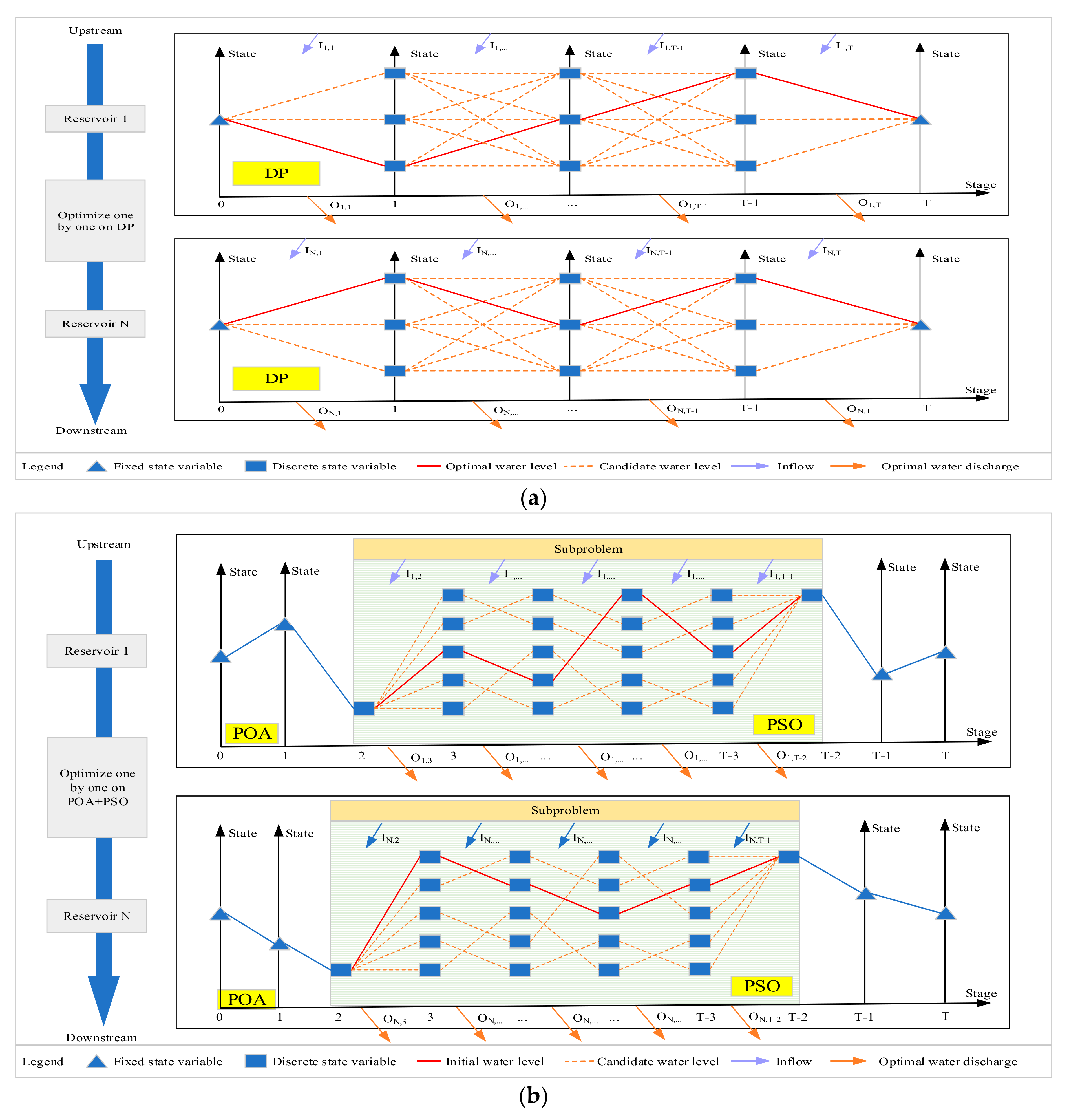
2.3.1. Dynamic Programming (DP)

DP is widely used in reservoir operation of hydropower generation, flood control, water storage, and so on. This paper uses DP to obtain the initial solution of reservoir operation. The recursive function of DP used in the multi-period optimal operation of the reservoir is described as Equation (10); DP is used to optimize reservoir operation from upstream to downstream. In this stage, the influence of river channel flood routing is not considered. The result of DP is used as the initial solution of the model.
min   G t Z n , t = g t Z n , t , Q n , t , o u t + G t 1 Z t 1 g t Z n , t , Q n , t , o u t = n = 1 N a n Z n u p Z n m i n Z n m a x Z n m i n + b n Q n , t , i n 2 + c n Q n , t , o u t 2 Q n , m a x 2 + m = 1 M d m Q m , t 2 Q m , m a x 2 + e m Q m , t , E Δ t t = 1 T Q m , t , E k Δ t s . t .   1   V n , t Z n , t + Q n , t , o u t Δ t = V n , t 1 Z n , t 1 + Q n , t , i n Δ t    2   Q m , t = h H Q h , m , t + Δ q m , t
where V n , t ( Z n , t ) is storage of the n-th reservoir at t-th period; G t ( Z n , t ) is the minimum cumulative utility from the G t ( Z n , t ) is the minimum cumulative utility from the first period (begin of operation period) to the t-th period (current operation period); g t ( Z n , t , Q n , t , o u t ) is the t-th period utility function, when the DP is used to optimize the operating water level of the n-th reservoir at t-th period, the operating water level in other periods remains unchanged, so only the utility value of the reservoir during the t-th period is calculated, which effectively reduces the amount of calculation [23]; Q h , m , t is the discharge of the h-th reservoir without considering the flood routing at the m-th point at the t-th period, Q h , m , t in Equation (7) that uses the Muskingum method for flood routing is simplified into Q h , m , t . The detailed steps at this stage are as follows:
Step 1: According to the operation requirements, the water level of the reservoirs is discretized into a water level sequence, and the discrete water level is set as a state variable. In this paper, the discrete step length of the reservoir is 0.01 meters.
Step 2: From upstream to downstream, the DP is used to optimize the reservoir operation process in turn.

2.3.2. Progressive Optimality Algorithm (POA)

POA can effectively avoid the “dimensional disaster” suffered by DP, and it can also consider the flood routing. On the basis of the initial solution, the multi-stage optimal operation problem is decomposed into a two-stage optimal operation sub-problem. The decision vector of sub-problem between the t-th and t+1-th period is described in Equation (11):
F ( Z n , t - 1 , Z n , t , Z n , t + 1 ) = m i n Z n , t C n , t { g t 1 ( Z n , t - 1 , Q n , t - 1 , o u t ) + g t ( Z n , t , Q n , t , o u t ) } s . t .   ( 1 )   V n , t ( Z n , t ) + Q n , t , o u t Δ t = V n , t - 1 ( Z n , t - 1 ) + Q n , t , i n Δ t    ( 2 )   Q m , t = h H Q h , m , t + Δ q m , t
where C n , t is the range that Z n , t can take at the t-th period and is determined by constraint 3, Q n , t - 1 , o u t and Q n , t , o u t are calculated by s.t.(1) using Z n , t - 1 , Z n , t , and Z n , t + 1 . F ( Z n , t - 1 , Z n , t , Z n , t + 1 ) is the optimal objective at the t-th and t+1-th period. The detailed steps at this stage are as follows [45,46]:
Step 1: Select the n-th reservoir from upstream to downstream for optimization calculation, and the operating water levels of other reservoirs remain unchanged.
Step 2: The water level of the n-th reservoir from the second period to the T−1-th period is optimized in turn. When the water level of the t-th period is optimized, the water level of the n-th reservoir remains unchanged in other periods, the optimization objective is shown in Equation (11).
Step 3: After optimizing the operation water level of the n-th reservoir is completed, the operating water level of the n + 1-th reservoir is optimized using the method in step 2.
Step 4: After optimizing the operation water levels of all reservoirs, repeat steps 1, 2, and 3 until the optimization results remain stable.

2.3.3. Particle Swarm Optimization (PSO)
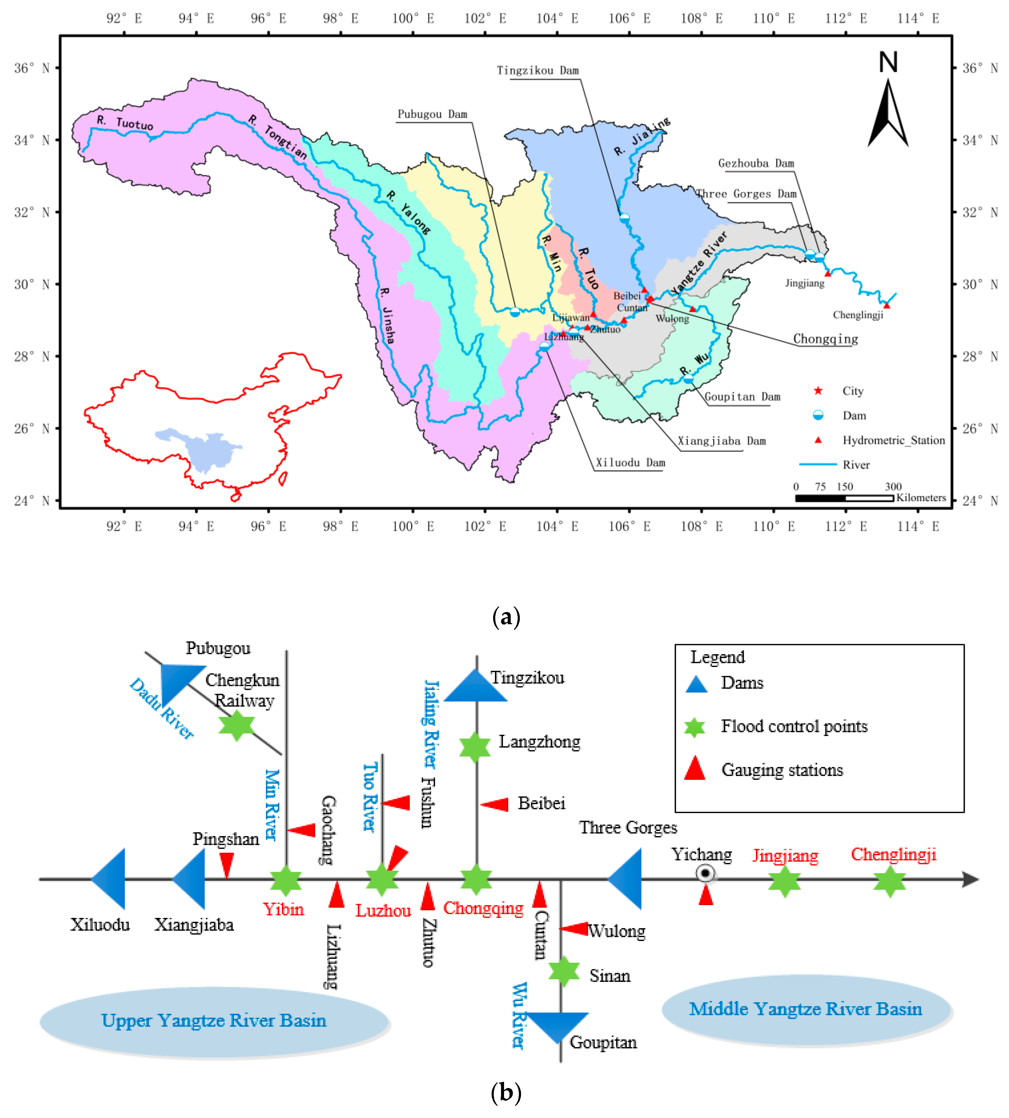
PSO is derived from the research on the predation behavior of bird swarms. Each particle in the particle swarm represents a possible solution to the problem. Through the simple behavior of individual particles, the information interaction within the particle swarm realizes the intelligence of problem solving. Due to its simple operation and fast convergence speed, PSO has been widely used in many fields such as function optimization, image processing, and geodesy [31]. The paper uses PSO to solve the problem that POA is easy to fall into local optimal solutions. However, if the optimization calculation is performed during the entire operation period, the length of the particles will be too long, thereby reducing the convergence speed. Therefore, this paper combines POA, and PSO, and selects several consecutive operation periods as the “operation window”. PSO is used to optimize the operation process in the “operation window”, and keeps the operation process in other periods unchanged. When the operation process optimization in the “operation window” is completed, the window moves backward and optimizes the operation process. Each particle in PSO evolves according to the set strategy. The formula for updating the velocity and position of the particles is as follows:
V i d ( r + 1 ) = w V i d ( r ) + C 1 r a n d o m ( 0 , 1 ) ( P i d X i d ( r ) ) + C 2 r a n d o m ( 0 , 1 ) ( P g d X i d ( r ) )
X i d ( r + 1 ) = X i d ( r ) + V i d ( r + 1 )
where X i d ( r ) is the position of the i-th particle in the r round of optimization, the value of X i d ( r ) in each dimension represents the operating water level of a reservoir in a period; V i d ( r ) is the velocity of the i-th particle with d dimensions in the r round of optimization, the value of V i d ( r ) in each dimension represents the change value of the operating water level of a reservoir in a period; P i d is the best position where the i-th particle has appeared so far; P g d is the best position where all particles have appeared so far; C 1 and C 2 are the learning constants; w is the weight of inertia; r a n d o m ( 0 , 1 ) is a random number between 0 and 1. The detailed steps at this stage are as follows [47,48,49]:
Step 1: Based on experience, the “operation window” is set to contain k periods. If k is set to be relatively large, the convergence speed will be slower. On the contrary, if k is set to be relatively small, the search ability will be reduced. The recommended interval is [10,30], and k is set to 20 in this paper;
Step 2: Set the number of particles, and initialize the velocity and position of particles. Each particle contains the water level of k periods of N reservoirs in the “operation window”, so the particle contains k × N dimensions. The result of POA in the “operation window” is used as one of the particles.
Step 3: According to the fitness function shown in Equation (14), calculate the fitness value of each particle.
F ( j , k ) = n = 1 N ( a n Z n u p - Z n m i n Z n m a x - Z n m i n + t = j j + k b n Q n , t , i n 2 + c n Q n , t , o u t 2 Q n , m a x 2 ) + m = 1 M ( t = j j + k d m Q m , t 2 Q m , m a x 2 + e m t = j j + k Q m , t , E Δ t t = 1 T Q m , t , E k Δ t )
where j is the starting period of the “operation window”. When optimizing the reservoir operating water level process in the “operation window” from the j-th period to the j+k-th period, the water levels in other periods remain unchanged, so only the periods in the window need to be considered when calculating the fitness. If j and k are set to 1 and T respectively, it can be discovered that this fitness function is the objective function.
Step 4: According to the fitness value of the particles, update the historical best position of each particle and the best position of the particle swarm [31].
Step 5: Update the velocity and position of each particle according to Equations (12) and (13).
Step 6: Repeat steps 3, 4, and 5 until the best position of the particle swarm remains stable.
Step 7: The “operation window” moves backward p periods, and the water level from the j+p-th period to the j+p+k-th period in the “operation window” is optimized. p is recommended not to be more than one-third of k, which is taken as 5 in this paper.

3. Study Area

3.1. Introduction of Study Area

The middle and upper Yangtze River is selected as a case study. As the largest river in China, the Yangtze River has a total length of about 6300 km. The area, population, GDP, and grain output of the Yangtze River Basin account for 18.8%, 36%, 40%, and 40% of the country respectively [50]. However, floods in the Yangtze River Basin often occur, killing thousands of people and causing millions of dollars in damage. For example, the flood of 1954 directly caused 30,000 deaths, and more people died of starvation and plague caused by the flood [51]. Therefore, flood control in the Yangtze River Basin has always been the focus of general attention, and flood prevention and disaster reduction in the Yangtze River Basin has been given top priority. The middle and upper Yangtze River are the most severely flooded areas and the key to flood control in the entire basin.
After decades of flood control construction, the Yangtze River Basin has basically formed a comprehensive flood control system with the Three Gorges Reservoir (TG) as the backbone. However, the contradiction between the river discharge capacity and the large flood peaks of the middle and lower reaches of the Yangtze River is still prominent. The 22.15 billion m3 flood control storage capacity of the TG only accounts for about 5% of the 451 billion m3 average annual runoff at the dam site. In extreme flood events, if only the Three Gorges Reservoir participates in flood control operation, the downstream flood diversion and storage area needs to be used, and the loss is very huge. Therefore, it is necessary for the upstream reservoirs to cooperate with the TG for joint flood control operation.
The flood control system consisting of key reservoirs and flood control points in the middle and upper Yangtze River is shown in Figure 3. The system includes six reservoirs including Xiluodu (XLD), Xiangjiaba (XJB), Pubugou (PBG), Tingzikou (TZK), Goupitan (GPT), Three Gorges (TG), and eight flood control stations including Chengkun Railway, Yibin, Luzhou, Chongqing, Langzhong, Sinan, Jingjiang, Chenglingji. In Figure 3b, Flood control point is the object that needs to be protected by the flood control operation of reservoirs, and the gauging station is the station for observing the water level and flow of the river.

3.2. Data of Study Area

3.2.1. Data of Reservoir

XLD is located in the lower reaches of the Jinsha River and is the third-largest hydropower station in the world. The height, total storage capacity, and flood control storage capacity of the dam are 285.5 meters, 12.67 billion m3, and 4.65 billion m3, respectively. XJB is located at the downstream of XLD, which is only 157 km far from it. The flood control storage capacity of XJB is 0.90 billion m3. The two reservoirs are key reservoirs of the Jinsha River, controlling 96% of the Jinsha River basin area.
PBG is a key reservoir in the Min River which is a tributary of the Yangtze River. It is located in the west of Sichuan Province and has a drainage area of 68,500 km2, accounting for about 50.4% of the Min River basin area. Its flood control storage capacity is 1.1 billion m3. TZK is a controlling water conservancy project of the Jialing River. It has a drainage area of 61,100 km2, accounting for 39% of the Jialing River basin area. The flood control water level and flood control storage capacity are 447 m and 1.44 billion m3, respectively. GPT is located in Guizhou Province and is the largest key reservoir on the Wu River. It controls a drainage area of 43,300 km2, accounting for 49% of the Wu River basin area. Its flood control storage capacity is 0.4 billion m3.
TG is located in Hubei Province and is the largest water conservancy project in the world. The length, height, total storage capacity, and flood control capacity of the dam are 3335 m, 181 m, 39.3 billion m3, and 22.15 billion m3 respectively. It is the key to flood control of the Yangtze River. The characteristics of the reservoirs are shown in Table 1.

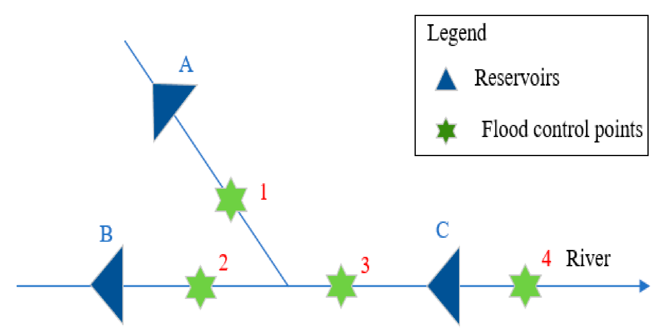
3.2.2. Data of Flood Control Point

The Chengkun Railway connects Sichuan Province and Yunnan Province with a total length of 1096 km. It is the most important transportation line in southwest China. According to the flood control standard stipulated by law, when the flow is not higher than 11,200 m3/s, which is the peak flow of the design flood with a return period of 100 years, PBG should be used to intercept the flow below 8780 m3/s, which is the maximum flow that the Chengkun Railway can withstand.
Yibin, Luzhou, and Langzhong are three cities located in Sichuan Province. The populations of the three cities are 5.5 million, 5.8 million, and 0.83 million respectively, and GDP are 37.7 billion, 31.1 billion, 3.7 billion dollars respectively. The current flood control capacity of the three cities is to ensure safety in the event of a flood with a return period of 20 years, the corresponding peak flows of the flood are 51,000 m3/s, 52,600 m3/s, and 25,100 m3/s, respectively. According to the flood control standard stipulated by law, upstream reservoirs should protect the three cities from the design flood with a return period of 50 years, the corresponding peak flow of the flood is 57,800 m3/s, 58,100 m3/s, and 32,880 m3/s.
Chongqing is the largest city in southwestern China and the center of economy, finance, science and technology, shipping, and logistics in the upper reaches of the Yangtze River. It has a population of 31.2 million, a GDP of 352.3 billion dollars, and an area of 82,400 km2. The discharge capacity of the river channel in Chongqing is 83,100 m3/s which is the peak flow of the design flood with a return period of 50 years, and the upstream reservoirs should protect Chongqing from the design flood with a return period of 100 years, the corresponding flood peak flow is 88,700 m3/s, according to the flood control standard stipulated by law.
Sinan is a county located in the northeast of Guizhou Province, with an area of 2230.5 km2, a population of 684,500, and a GDP of 2 billion dollars. According to the flood control standard stipulated by law, when the flow is not higher than 11,500 m3/s which is the peak flow of the design flood with return period of 5 years, GPT should be used to intercept the flow below 9320 m3/s which is the peak flow of the design flood with a return period of 2 years.
Jingjiang is an important production base for grain, cotton, oil, fruits, and aquatic products in China. It has a population of 9.6 million, 16.6 million acres of arable land, many important railways and highways. Once floods occur, they will directly threaten the safety of Wuhan which is the most important city in central China. On the other hand, the flood discharge capacity of the Jingjiang is only 60,600 m3/s, which is seriously insufficient compared to the huge amount of inflow. Therefore, the Jingjiang River has always been the difficulty and focus of the Yangtze River flood control. Chenglingji is located in Yueyang City, Hunan Province. It is the exit of Dongting Lake into the Yangtze River. Chenglingji is the area where flood disasters occur most frequently in the Yangtze River Basin.
In this flood control system, the flood control objectives of the Chengkun Railway, Yibin, Luzhou, Chongqing, Langzhong, and Sinan are transformed into constraints to ensure that they meet the flood control standards. Then, this paper focus on solving the flood control problems of Jingjiang and Chenglingji.

3.2.3. Muskingum Parameters of the Basin

The Muskingum parameters of each reach in the basin are shown in Table 2. The flood routing time of each river segment is 6 h.

4. Application

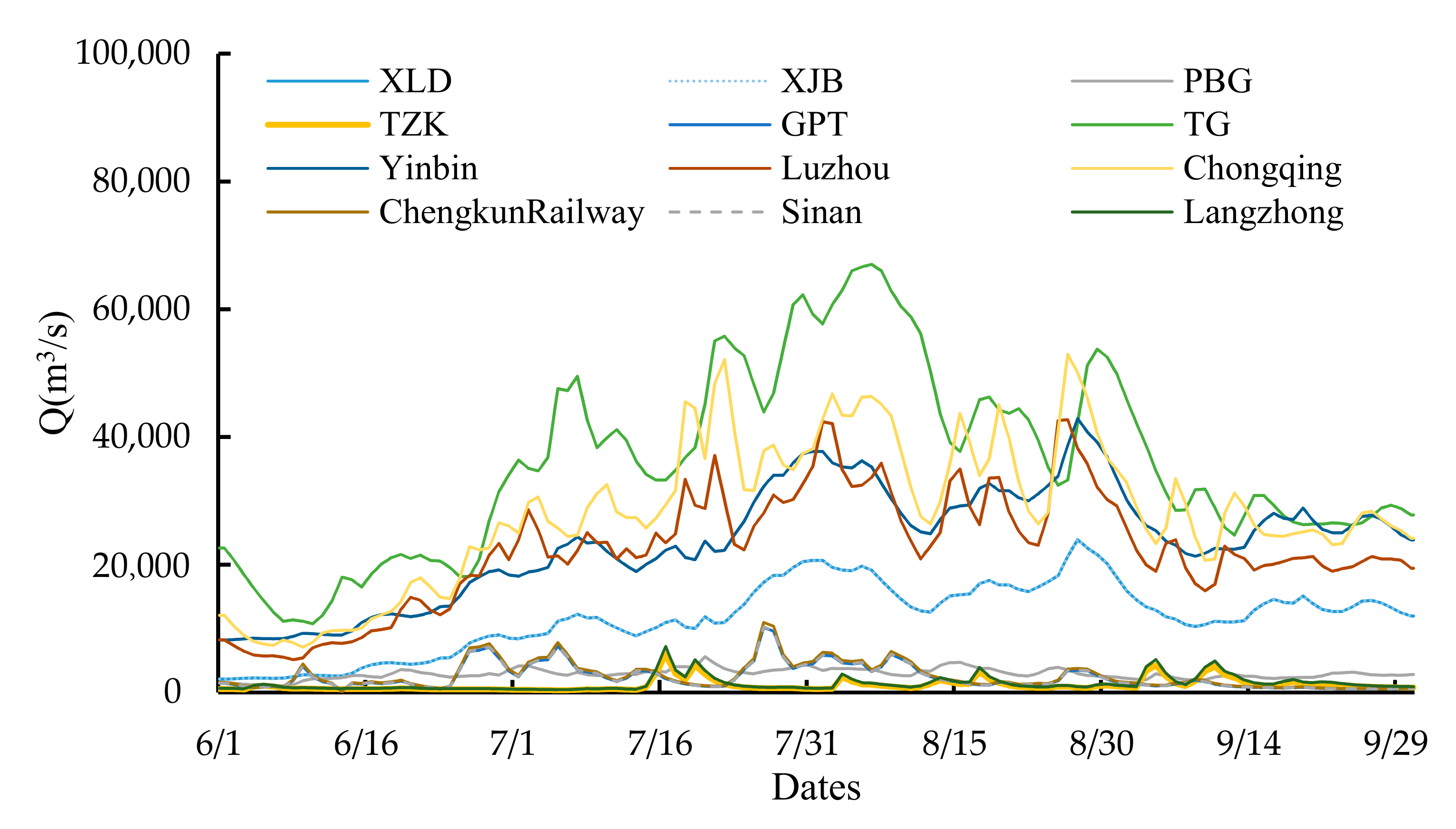
4.1. Design Flood Hydrographs

The flood control operation of the reservoirs is to ensure the safety when a large or extreme flood occurs [52]. The common method is to determine the flood control standard based on the importance of the flood control point, and then the design flood corresponding to the standard is used as the input of the operation model [28,53]. There are two methods commonly used in design flood calculation: homogeneous frequency enlargement and homogeneous multiple enlargement. The homogeneous frequency enlargement is widely used in the case of a large number of reservoirs and flood control points because of its ease of use [54,55,56]. The steps of this method to calculate the design flood are as follows:
Step 1: The design flood parameters of the control section are obtained by calculating the frequency of the annual maximum flood peak and n-day volumes data. The control section of this study is the Yichang gauging station, and its design flood parameters are shown in Table 3. In the table, Ex, Cv, and Cs are the mean value, coefficient of variation, and coefficient of skewness of design flood respectively [54].
Step 2: The typical flood hydrographs were determined. An observed flood hydrograph with a large peak, large flood volume, or an operation not conducive to flood control was usually selected [57]. This study selected floods in 1954, 1968, 1980, 1981, 1982, 1988, 1996, 1998, 1999, and 2010 as a typical flood hydrograph. The 1954 and 1998 floods were respectively the first and second largest floods in the Yangtze River in the 20th century, and caused serious disasters to the entire basin. Large floods occurred in the middle reach of the Yangtze River in 1968, 1988, and 1999. The 1980 flood caused severe flood disasters to the Jinsha River and Jialing River, which are tributaries of the Yangtze River. In 1981, the Jinsha River, the Minjiang River, and the Jialing River experienced large floods at the same time, which put great pressure on flood control safety. In 1982, The largest flood in history occurred in Tuojiang which is a tributary of the Yangtze River. In 2010, the Minjiang River and the Jialing River experienced large floods at the same time, and the flood peak of the Cuntan gauging station reached 64,000 m3/s. The 11 selected typical flood hydrographs can represent the worst flood characteristics in the middle and upper Yangtze River.
Step 3: The design flood hydrographs were determined. According to the ratio of the peak or n-day volumes between the observed typical flood and the design flood at the control section, the typical flood hydrographs of reservoirs and flood control points in the basin are enlarged and become the basin design flood hydrographs. Usually, the flood volume ratio close to the peak ratio is selected for enlarging to ensure that the flood peak and flood volume of the design flood match. In this study, the 1954 and 1998 floods used the ratio of 30-day volume, and other floods used the ratio of 15-day volume.
The start time and end time of the design flood are June 1 and September 30, respectively. Due to space limitations, this study only shows the 1954 and 1998 typical year design flood with return period of 100-year, as shown in Figure 4 and Figure 5, respectively.

4.2. Optimal Reservoir Operation Results

In this study, a joint flood control optimal operation model of the flood control system composed of six reservoirs and eight points in the upper and middle reaches of the Yangtze River was established, and 1954, 1968, 1980, 1981, 1982, 1988, 1996, 1998, 1999, and 2010 typical year design floods with different return periods were used as the inputs of the model. Then, the DP-POA-PSO proposed in this paper is used to solve the optimal model. The system has three main flood control goals: first, the flood diversion volumes of Jingjiang is reduced to the lowest; second, the flood diversion volumes of Chenglingji is reduced to the lowest; third, the highest operation water level of TG is the lowest. The importance of the three goals decreases in order. The programming tool, programming language, and database use eclipse, java, and MySQL respectively. On a computer with a CPU frequency of 4.0 GHz, the calculation time of using this algorithm to solve the model is about 180 s.

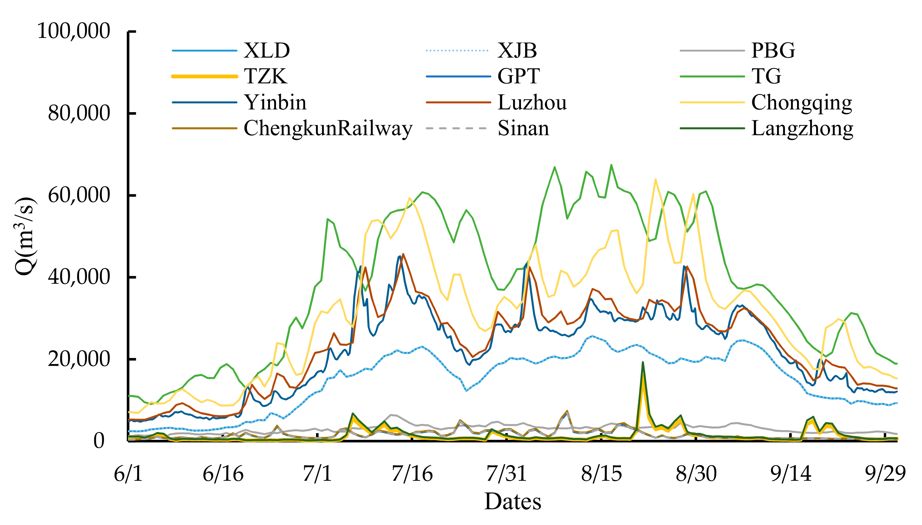
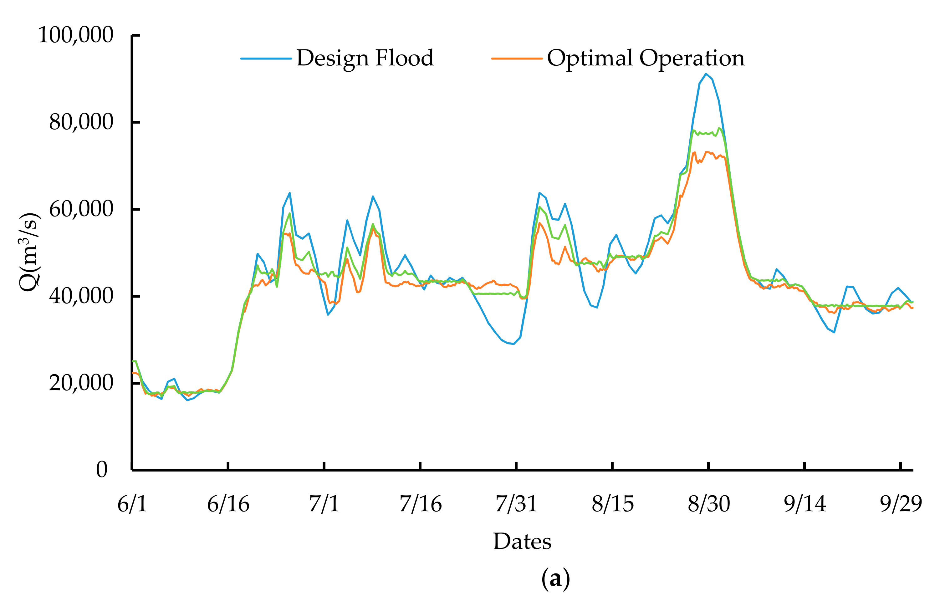
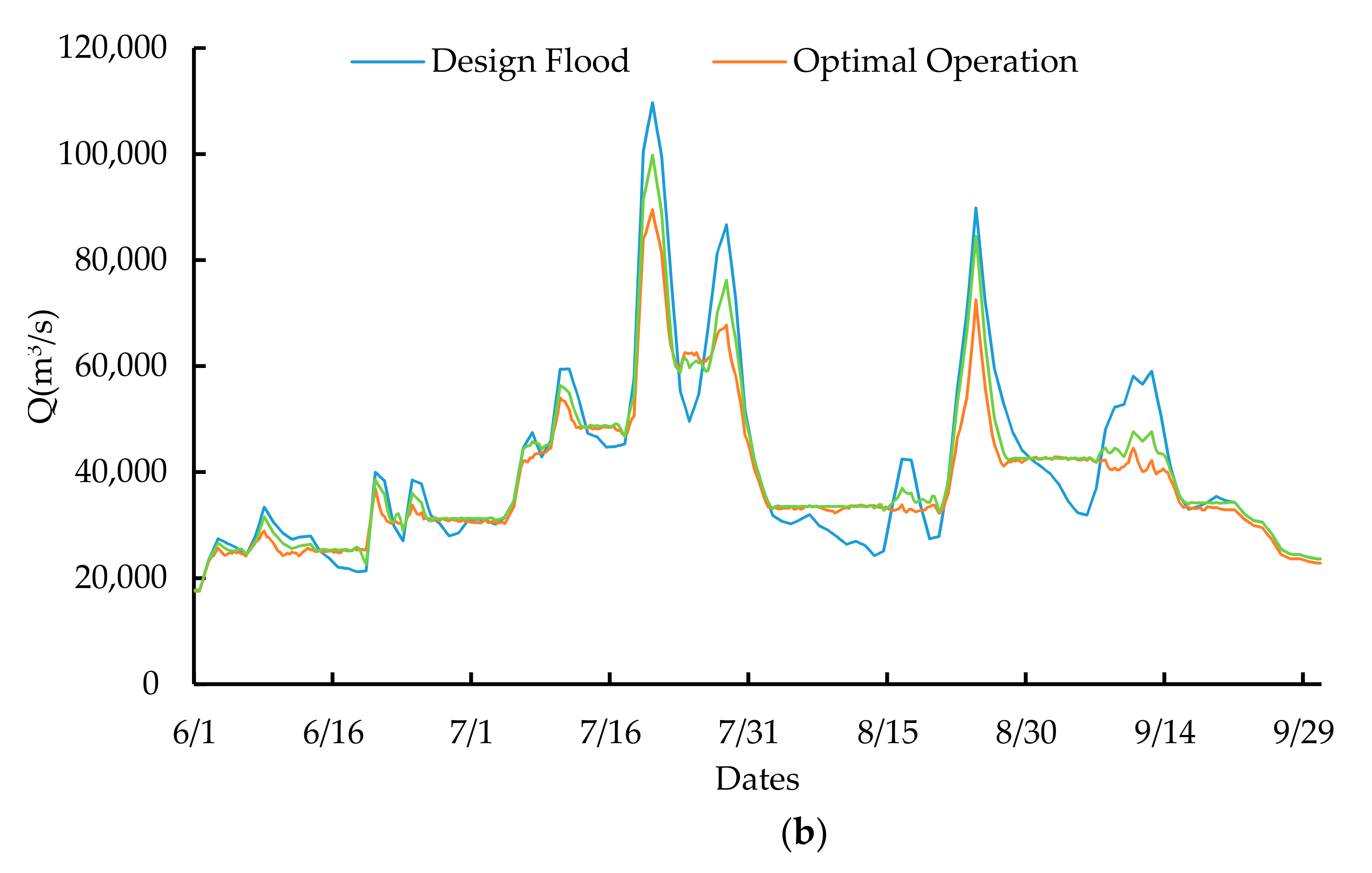
4.2.1. Influence on the Inflow Flood of TG

The operation of the upstream reservoir can reduce the inflow flood of the TG. The operation results of this part are shown in Table 4. In the current method, each reservoir is operated separately and no joint optimal operation is realized. In the table, the design value is the inflow peak of TG without reservoir operation; the reduction is the difference between the design value and the inflow peak after reservoir operation; the comparison is the difference between the peak flows of the current method and the optimal operation.
The operation results show that the joint optimal operation of the reservoirs can make full use of the flood control capacity of the upstream reservoirs to reduce the inflow of TG and reduce its flood control pressure. Therefore, the flood control effect of TG on Jingjiang and Chenglingji has been greatly improved. For the designed floods with return periods of 1000 years, 100 years, and 50 years, compared with the current method, the optimal operation increases the inflow peak reduction by 68%, 37% and 36%, respectively. Figure 6 shows the inflow of TG when different methods are used to operate the 1980 and 2010 typical year design flood with a return period of 1000 years. The results show that the joint optimal operation can make the inflow flatter and the peak smaller, which will increase the flexibility of TG for flood control operation of Jingjiang and Chenglingji.

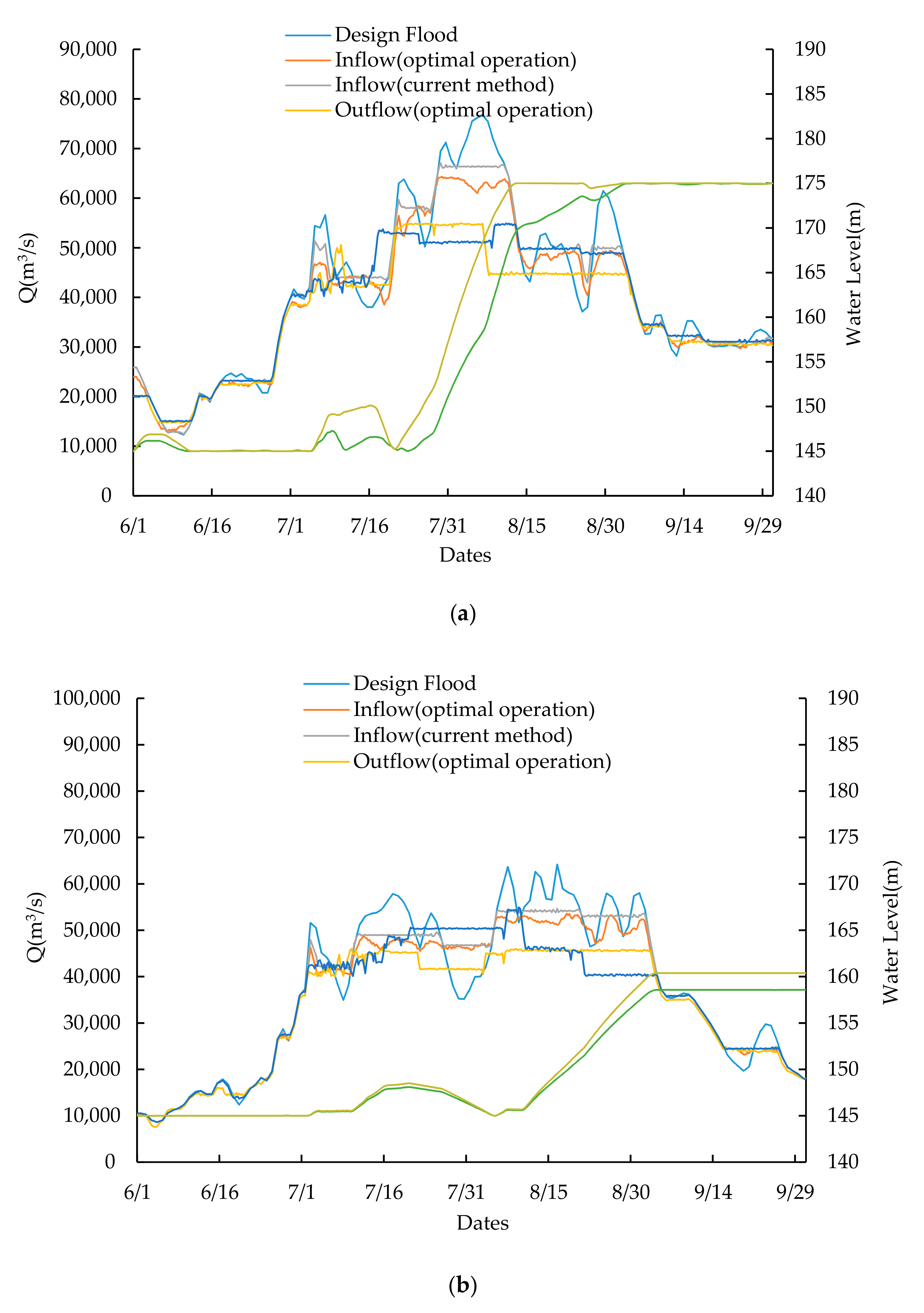
4.2.2. Operation Results of Jingjiang and Chenglingji

Considering that the Chengkun Railway, Yibin, Luzhou, Langzhong, and Sinan can all meet the flood control standards after reservoir operation, many studies [58,59,60,61] have been focusing on the operation effect of the reservoir group on Jingjiang and Chenglingji, especially the flood diversion of these two areas. In order to prove the feasibility of the optimal flood control operation model and DP-POA-PSO algorithm proposed in this paper, the results of the optimal operation model are compared with the current methods. The flood diversions in Jingjiang and Chenglingji are shown in Table 5 and Table 6, respectively.
The Table 5 show that the flood control optimal operation model of reservoirs can greatly improve the flood control safety of the Jingjiang. When floods with return period of 50 or 100 years occur, the flow after the reservoir operation does not exceed the discharge capacity of the Jingjiang, and there is no need to use the flood diversion areas. In the event of the flood with return period of 1000 years, the optimized model reduced Jingjiang’s flood diversion volumes by 25.3 billion m3 on average, especially the flood diversion volume of the 2010 design floods reduced by 48.8 billion. Compared with the current method, the Jingjiang flood diversion volumes has been reduced by 1.78 billion m3 on average.
On the other hand, Table 6 shows that the flood control safety of Chenglingji area has also been greatly improved. In the event of floods with return period of 50 years, there is no need to use the flood diversion areas in Chenglingji, this will greatly reduce the pressure of flood diversion in Chenglingji. Compared with the current method, the Chenglingji’s flood diversion volumes has been reduced by 0.16, 0.25, and 1.96 billion m3 respectively on average when floods with return period of 50, 100, and 1000 years occur.
From the operation results of Jingjiang and Chenglingji, it can be seen that the flood control optimal operation model of reservoirs and DP-POA-PSO algorithm proposed in this paper can significantly reduce the flood diversion of these two flood control points compared with the current method. When the flood is not large, the goal of no flood diversion can be achieved, which will greatly reduce the flood disaster loss.

4.2.3. Operation Results of TG

The highest operating water level of TG is shown in Table 7. The lower water level can reduce the flood control risk of the reservoir itself and increase the flexibility of flood control operation. Compared with the current method, the water level has been reduced by 1.72, 1.58, and 0.38 m respectively on average when floods with return period of 50,100, and 1000 years occur. In the event of a flood with a return period of 1000 years, the maximum highest water level is 175 m, and the minimum highest water level is 171.51 m. These results show that the flood control capacity of the reservoir is fully used in order to reduce the flood diversion of Jingjiang and Chenglingji when a large flood occurs. Conversely, when the flood with return period of 50 years occur, the maximum and minimum highest water level are 166.24, 158.57 m, respectively. These results show that when the flood is not large, the highest water level of the reservoir is reduced as much as possible under the premise of ensuring the minimum flood diversion volumes of Jingjiang and Chenglingji to reduce the flood control risk of the reservoir itself.
Figure 7 shows the results of the TG under different operation methods, using as the designed flood the 1954 typical year with return periods of 50 and 1000 years. The figure shows that the results obtained by the optimal operation model are usually better than that of the current method, because inflow and outflow of TG are much smaller and much flatter. In particular, the operation water level of TG is also lower.
It can be seen from Table 4, Table 5, Table 6 and Table 7 that for 10 design floods with different encounter characteristics, the model and algorithm proposed in this paper can effectively reduce the peak inflow of the reservoir, the highest operating water level of the reservoir, and the flood diversion of flood control points. On the other hand, when the flood is large, the goal of reducing the amount of flood diversion is achieved. When the flood is small, the operating water level of the reservoir is further reduced, and the flood control risk of the reservoir itself is reduced. These show that the method has good adaptability.

5. Conclusions and Discussion

In this study, a joint flood control optimal operation model with multiple reservoirs and flood control points was established, which gave full play to the flood control potential of the reservoirs, and balanced the flood control demand between reservoirs and flood control points. The impact of transposition and attenuation of flood cannot be ignored, so the Muskingum routing method is used by the operation model. A DP-POA-PSO optimization algorithm is proposed to solve the optimal operation model. Then, a flood control system consisting of six reservoirs and eight flood control points in the middle and upper Yangtze River is selected as a case study. The study mainly aims at minimizing the flood diversion volumes of Jingjiang and Chenglingji, the maximum inflow of TG and the highest operating water level of TG. The main conclusions are summarized as follows.
(1) This article has two main innovations. The first innovation is that an optimal operation model for multiple reservoirs and flood control points was proposed. The flood control potentiality of the reservoirs is fully utilized, and the flood loss and risk of the system are significantly reduced. In addition, compared with simplified methods such as time delay, the use of the Muskingum method makes the river channel flood routing more accurate, which makes the operation result more in line with the actual project. The second innovation is the proposed DP-POA-PSO optimization algorithm, which combines the advantages of each algorithm in solving the optimal operation of the reservoir, avoiding the “dimensional disaster”, local optimal solution, slow convergence speed, and so on. It shows excellent performance in practical applications.
(2) The optimal operation model and algorithm proposed in this paper can significantly reduce the inflow of the Three Gorges Reservoir. For the design flood with return periods of 1000 years, 100 years, and 50 years, the average reduction of inflow peak is 13,311 m3/s, 10,258 m3/s, and 10,027 m3/s, respectively, the corresponding rate of reduction is 14.6%,13.0%, and 13.4% respectively. Compared with the current method, the optimal operation increases the inflow peak reduction by 5375 m3/s, 2794 m3/s, and 2628 m3/s respectively.
(3) The joint flood control optimal operation of reservoirs can greatly improve the flood control safety of Jingjiang and Chenglingji. When floods with return period of 50 or 100 years occur, the flow after the reservoir operation does not exceed the discharge capacity of the Jingjiang, and there is no need to use the flood diversion areas. In the event of a flood with a return period of 1000 years, the optimized model reduced Jingjiang’s flood diversion volumes by 25.3 billion m3 on average. Compared with the current method, the Jingjiang flood diversion volume has been reduced by 1.78 billion m3 on average. On the other hand, in the event of a flood with a return period of 50 years, there is no need to use the flood diversion areas in Chenglingji, this will greatly reduce the pressure of flood diversion in Chenglingji. Compared with the current method, Chenglingji’s flood diversion volumes have been reduced by 0.16, 0.25, and 1.96 billion m3 respectively on average when floods with return period of 50,100, and 1000 years occur.
(4) The results show that the optimal operation model has good adaptability and flexibility. When a large flood occurs, the flood control capacity of the reservoir is fully used in order to reduce the flood diversion of Jingjiang and Chenglingji. Conversely, when the flood is not large, the highest water level of Three Gorges Reservoir is reduced as much as possible under the premise of ensuring the minimum flood diversion volumes of Jingjiang and Chenglingji to reduce the flood control risk of the reservoir itself.
In real-time flood operation, the inflow at each point in the basin can be obtained through forecasting, and then the model and algorithm proposed in this paper are used to operate the forecasted inflow. The operation results can provide program support for real-time flood control operation. In addition, the operation results of design floods can provide guidance for the formulation of the joint flood control operation rules of reservoirs and flood control points. It can be seen from the operation results that although the operation of the six reservoirs has reduced the flood diversion volumes of Chenglingji, the flood control pressure is still very high, so more reservoirs and more efficient algorithms need to be considered to solve this problem.
In addition, there are many uncertain factors in the operation, which will affect the flood control effect of reservoirs. Research by Hu et al. [62], Krzysztofowicz et al. [63], Chen et al. [64], and Vermuyten et al. [65] showed that among all the uncertain factors in flood control operation, the uncertainty of flood forecast has the greatest impact on operation results, especially in long-term operation. The uncertainty of the forecast mainly includes three aspects: the error of inflow, the error of flood volume, and the error of flood hydrograph shape. At the same time, the water level-storage curve and the water level-discharge capacity of reservoir curve also have an influence on operation [65]. In order to reduce the difficulty of model solving and increase the speed of calculation, this study did not consider these uncertain factors. Uncertainty can be considered in future research to further improve the operation effect.

Author Contributions

G.Z. designed and conducted the experiments. G.Z., X.Y., and W.F. wrote the draft of the paper. J.Z. proposed the main structure of this study. L.D., Q.W., and X.D. provided useful advice and made some corrections. All authors have read and agreed to the published version of the manuscript.

Funding

This research was funded by the National Key R&D Program of China (No. 2016YFC0402205, No. 2017YFC0405900); the National Natural Science Foundation of China (No. 51679094, No. 52039004); the National Natural Science Foundation Key Project of China (No. 91547208) and the Foundation of Huazhong University of Science and Technology (No. 2017KFYXJJ209).

Institutional Review Board Statement

Not applicable.

Informed Consent Statement

Not applicable.

Data Availability Statement

Data sharing not applicable.

Conflicts of Interest

The authors declare no conflict of interest.

References

  1. Chen, C.; Yuan, Y.; Yuan, X. An Improved NSGA-III Algorithm for Reservoir Flood Control Operation. Water Resour. Manag. 2017, 31, 4469–4483. [Google Scholar] [CrossRef]
  2. Zhang, W.; Liu, P.; Chen, X.; Wang, L.; Ai, X.; Feng, M.; Liu, D.; Liu, Y. Optimal Operation of Multi-reservoir Systems Considering Time-lags of Flood Routing. Water Resour. Manag. 2015, 30, 523–540. [Google Scholar] [CrossRef]
  3. Zhou, Y.; Guo, S.; Liu, P.; Xu, C. Joint operation and dynamic control of flood limiting water levels for mixed cascade reservoir systems. J. Hydrol. 2014, 519, 248–257. [Google Scholar] [CrossRef]
  4. Qin, H.; Zhou, J.; Lu, Y.; Li, Y.; Zhang, Y. Multi-objective Cultured Differential Evolution for Generating Optimal Trade-offs in Reservoir Flood Control Operation. Water Resour. Manag. 2010, 24, 2611–2632. [Google Scholar] [CrossRef]
  5. Reddy, M.J.; Kumar, D.N. Optimal Reservoir Operation Using Multi-Objective Evolutionary Algorithm. Water Resour. Manag. 2006, 20, 861–878. [Google Scholar] [CrossRef] [Green Version]
  6. Liu, X.; Chen, L.; Zhu, Y.; Singh, V.P.; Qu, G.; Guo, X. Multi-objective reservoir operation during flood season considering spillway optimization. J. Hydrol. 2017, 552, 554–563. [Google Scholar] [CrossRef]
  7. Yazdi, J.; Neyshabouri, S.A.A.S. Optimal design of flood-control multi-reservoir system on a watershed scale. Nat. Hazards 2012, 63, 629–646. [Google Scholar] [CrossRef]
  8. Xiaocong, H.; Lisheng, Z.; Linyun, L. Study on flood control operation of Jinsha River cascade reservoirs combined with the Three Gorges along the Yangtze River. IOP Conf. Ser.: Mater. Sci. Eng. 2017, 199, 12032. [Google Scholar] [CrossRef] [Green Version]
  9. Lee, S.Y.; Hamlet, A.F.; Fitzgerald, C.J.; Burges, S.J. Optimized Flood Control in the Columbia River Basin for a Global Warming Scenario. J. Water Resour. Plan. Manag. 2009, 135, 440–450. [Google Scholar] [CrossRef] [Green Version]
  10. Chou, F.N.-F.; Wu, C.-W. Stage-wise optimizing operating rules for flood control in a multi-purpose reservoir. J. Hydrol. 2015, 521, 245–260. [Google Scholar] [CrossRef]
  11. Guo, S.; Chen, J.; Li, Y.; Liu, P.; Li, T. Joint Operation of the Multi-Reservoir System of the Three Gorges and the Qingjiang Cascade Reservoirs. Energies 2011, 4, 1036–1050. [Google Scholar] [CrossRef] [Green Version]
  12. Chang, L.-C.; Chang, F.-J. Multi-objective evolutionary algorithm for operating parallel reservoir system. J. Hydrol. 2009, 377, 12–20. [Google Scholar] [CrossRef]
  13. Li, X.; Guo, S.; Liu, P.; Chen, G. Dynamic control of flood limited water level for reservoir operation by considering inflow uncertainty. J. Hydrol. 2010, 391, 124–132. [Google Scholar] [CrossRef]
  14. Ouyang, S.; Zhou, J.; Li, C.; Liao, X.; Wang, H. Optimal design for flood limit water level of cascade reservoirs. Water Resour. Manag. 2015, 29, 445–457. [Google Scholar] [CrossRef]
  15. Chen, J.; Guo, S.; Li, Y.; Liu, P.; Zhou, Y. Joint Operation and Dynamic Control of Flood Limiting Water Levels for Cascade Reservoirs. Water Resour. Manag. 2013, 27, 749–763. [Google Scholar] [CrossRef]
  16. Unver, O.I.; Mays, L.W. Model for real-time optimal flood control operation of a reservoir system. Water Resour. Manag. 1990, 4, 21–46. [Google Scholar] [CrossRef]
  17. Wei, C.C.; Hsu, N.S. Multireservoir Flood-Control Optimization with Neural-Based Linear Channel Level Routing Under Tidal Effects. Water Resour. Manag. 2008, 22, 1625–1647. [Google Scholar] [CrossRef]
  18. Xin-Yu, W.; Ping-An, Z.; Xuan, C.; Li, D.; Ben-You, J. Computer Simulation of Flood Scheduling in Large Scale Flood Control Systems. Procedia Eng. 2012, 29, 3267–3275. [Google Scholar] [CrossRef] [Green Version]
  19. Zhou, C.; Sun, N.; Chen, L.; Ding, Y.; Zhou, J.; Zha, G.; Luo, G.; Dai, L.; Yang, X. Optimal operation of cascade reservoirs for flood control of multiple areas downstream: A case study in the upper Yangtze river basin. Water 2018, 10, 1250. [Google Scholar] [CrossRef] [Green Version]
  20. Moridi, A.; Yazdi, J. Optimal Allocation of Flood Control Capacity for Multi-Reservoir Systems Using Multi-Objective Optimization Approach. Water Resour. Manag. 2017, 31, 4521–4538. [Google Scholar] [CrossRef]
  21. Zhou, Y.; Guo, S.; Chang, L.-C.; Liu, P.; Chen, A.B. Methodology that improves water utilization and hydropower generation without increasing flood risk in mega cascade reservoirs. Energy 2018, 143, 785–796. [Google Scholar] [CrossRef]
  22. Hall, W.A.; Butcher, W.S.; Esogbue, A. Optimization of the Operation of a Multiple-Purpose Reservoir by Dynamic Programming. Water Resour. Res. 1968, 4, 471–477. [Google Scholar] [CrossRef]
  23. Jiang, Z.; Qin, H.; Ji, C.; Feng, Z.; Zhou, J. Two Dimension Reduction Methods for Multi-Dimensional Dynamic Programming and Its Application in Cascade Reservoirs Operation Optimization. Water 2017, 9, 634. [Google Scholar] [CrossRef] [Green Version]
  24. Jiang, Z.; Ji, C.; Qin, H.; Feng, Z. Multi-stage progressive optimality algorithm and its application in energy storage operation chart optimization of cascade reservoirs. Energy 2018, 148, 309–323. [Google Scholar] [CrossRef]
  25. Nanda, J.; Bijwe, P.R. Optimal Hydrothermal Scheduling with Cascaded Plants Using Progressive Optimality Algorithm. IEEE Trans. Power Appar. Syst. 1981, 100, 2093–2099. [Google Scholar] [CrossRef]
  26. Liu, P.; Cai, X.; Guo, S. Deriving multiple near-optimal solutions to deterministic reservoir operation problems. Water Resour. Res. 2011, 47, 2168–2174. [Google Scholar] [CrossRef]
  27. Windsor, J.S. Optimization model for the operation of flood control systems. Water Resour. Res. 1973, 9, 1219–1226. [Google Scholar] [CrossRef]
  28. Brandao, J.L.B. Performance of the Equivalent Reservoir Modelling Technique for Multi-Reservoir Hydropower Systems. Water Resour. Manag. 2010, 24, 3101–3114. [Google Scholar] [CrossRef]
  29. Chuanwen, J.; Bompard, E. A self-adaptive chaotic particle swarm algorithm for short term hydroelectric system scheduling in deregulated environment. Energy Convers. Manag. 2005, 46, 2689–2696. [Google Scholar] [CrossRef]
  30. Ostadrahimi, L.; Marino, M.A.; Afshar, A. Multi-reservoir Operation Rules: Multi-swarm PSO-based Optimization Approach. Water Resour. Manag. 2011, 26, 407–427. [Google Scholar] [CrossRef]
  31. Wang, W.; Lin, Q. Optimal Reservoir Operation Using PSO with Adaptive Random Inertia Weight. In Proceedings of the 2010 International Conference on Artificial Intelligence and Computational Intelligence, Sanya, China, 23–24 October 2010. [Google Scholar]
  32. Kumphon, B. Genetic Algorithms for Multi-objective Optimization: Application to a Multi-reservoir System in the Chi River Basin, Thailand. Water Resour. Manag. 2013, 27, 4369–4378. [Google Scholar] [CrossRef]
  33. Moreira, R.M.M. Simulation–Optimization Modeling: A Survey and Potential Application in Reservoir Systems Operation. Water Resour. Manag. 2010, 24, 1107–1138. [Google Scholar]
  34. Reis, L.F.R.; Walters, G.A.; Savic, D.; Chaudhry, F.H. Multi-Reservoir Operation Planning Using Hybrid Genetic Algorithm and Linear Programming (GA-LP): An Alternative Stochastic Approach. Water Resour. Manag. 2005, 19, 831–848. [Google Scholar] [CrossRef]
  35. Reddy, M.J.; Kumar, D.N. Multiobjective Differential Evolution with Application to Reservoir System Optimization. J. Comput. Civ. Eng. 2007, 21, 136–146. [Google Scholar] [CrossRef]
  36. Qian, W.; Li, A. Adaptive differential evolution algorithm for multiobjective optimization problems. Appl. Math. Comput. 2008, 201, 431–440. [Google Scholar] [CrossRef]
  37. Zhang, J.; Wang, X.; Liu, P.; Lei, X.; Li, Z.; Gong, W.; Duan, Q.; Wang, H. Assessing the weighted multi-objective adaptive surrogate model optimization to derive large-scale reservoir operating rules with sensitivity analysis. J. Hydrol. 2017, 544, 613–627. [Google Scholar] [CrossRef]
  38. Sun, P.; Wang, L.P.; Jiang, Z.Q.; Ji, C.M.; Zhang, Y.K. Application of two multi-dimensional dynamic programming algorithms in optimization of cascade reservoirs operation. J. Hydraul. Eng. 2014, 45, 1327–1335. [Google Scholar]
  39. Zong, H.; Li, C.; Zhou, J. Research and application for short-time cascaded hydroelectric scheduling based on progressive optimality algorithm. Hydroelectr. Energy 2003, 21, 46–48. [Google Scholar]
  40. Wen, X.; Zhou, J.; He, Z.; Wang, C. Long-Term Scheduling of Large-Scale Cascade Hydropower Stations Using Improved Differential Evolution Algorithm. Water 2018, 10, 383. [Google Scholar] [CrossRef] [Green Version]
  41. Azamathulla, H.M.; Wu, F.C.; Ghani, A.A.; Narulkar, S.M.; Zakaria, N.A.; Chang, C.K. Comparison between genetic algorithm and linear programming approach for real time operation. J. Hydro-Environ. Res. 2008, 2, 172–181. [Google Scholar] [CrossRef]
  42. Gill, M.A. Flood routing by the Muskingum method. J. Hydrol. 1978, 36, 353–363. [Google Scholar] [CrossRef]
  43. Tung, Y.K. River Flood Routing by Nonlinear Muskingum Method. J. Hydraul. Eng. 1985, 111, 1447–1460. [Google Scholar] [CrossRef] [Green Version]
  44. Jia, B.; Zhong, P.; Wan, X.; Xu, B.; Chen, J. Decomposition–coordination model of reservoir group and flood storage basin for real-time flood control operation. Hydrol. Res. 2015, 46, 11–25. [Google Scholar] [CrossRef]
  45. Xubao, Q. Research for Optimal Flood Dispatch Model for Reservoir Based on POA. Water Resour. Power 2008, 4, 35–37. [Google Scholar]
  46. Afshar, M.H. Large scale reservoir operation by Constrained Particle Swarm Optimization algorithms. J. Hydro-Environ. Res. 2012, 6, 75–87. [Google Scholar] [CrossRef]
  47. He, Y.; Xu, Q.; Yang, S.; Liao, L. Reservoir flood control operation based on chaotic particle swarm optimization algorithm. Appl. Math. Model. 2014, 38, 4480–4492. [Google Scholar] [CrossRef]
  48. Tayfur, G. Modern Optimization Methods in Water Resources Planning, Engineering and Management. Water Resour. Manag. 2017, 31, 3205–3233. [Google Scholar] [CrossRef]
  49. Fang, H.; Han, D.; He, G.J.; Chen, M. Flood management selections for the Yangtze River midstream after the Three Gorges Project operation. J. Hydrol. 2012, 432–433, 1–11. [Google Scholar] [CrossRef]
  50. Gang, Z. Preliminary study on the causes and countermeasures of the 1954 and 1998 extraordinary Yangtze river floods. J. Catastrophol. 1999, 4, 43–44. [Google Scholar]
  51. Huang, W.C.; Hsieh, C.L. Real-time reservoir flood operation during typhoon attacks. Water Resour. Res. 2010, 46, 759–768. [Google Scholar] [CrossRef]
  52. Yue, S.; Ouarda, T.B.M.J.; Bobée, B.; Legendre, P.; Bruneau, P. Approach for Describing Statistical Properties of Flood Hydrograph. J. Hydrol. Eng. 2002, 7, 147–153. [Google Scholar] [CrossRef]
  53. Faulkner, D.S.; Barber, S. Performance of the Revitalised Flood Hydrograph method. J. Flood Risk Manag. 2009, 2, 254–261. [Google Scholar] [CrossRef]
  54. Pramanik, N.; Panda, R.K.; Sen, D. Development of design flood hydrographs using probability density functions. Hydrol. Process. 2010, 24, 415–428. [Google Scholar] [CrossRef]
  55. Yi, X.; Guo, S.; Pan, L.; Yan, B.; Lu, C. Design Flood Hydrograph Based on Multicharacteristic Synthesis Index Method. J. Hydrol. Eng. 2009, 14, 1359–1364. [Google Scholar]
  56. Chen, L.; Guo, S.; Yan, B.; Liu, P.; Fang, B. A new seasonal design flood method based on bivariate joint distribution of flood magnitude and date of occurrence. Hydrol. Sci. J. 2010, 55, 1264–1280. [Google Scholar] [CrossRef] [Green Version]
  57. Li, J.B.; Guo, Y.C.; Zhao, Z.H.; Shuai, H.; Xie, L. Impact of the Three Gorges Reservoir Flood Prevention Dispatching Tohydrologic Information and Disaster Information in Dongting Lake Area. Adv. Mater. Res. 2012, 518, 3652–3661. [Google Scholar] [CrossRef]
  58. Liu, X.; Qu, G.; Guo, X.; Yue, H. Study on the Three Gorges reservoir flood control operation chart considering comprehensive utilization requirements. IOP Conf. Ser. Earth Environ. Sci. 2019, 304, 042040. [Google Scholar] [CrossRef] [Green Version]
  59. Yan, Z. Thinking on the flood disaster in the middle reaches of the Yangtze river. Earth Sci. Front. 2000, 7, 87–93. [Google Scholar]
  60. Zhenzhen, W.; Wei, S. Great Flood Water and Disaster Years of Dongting Lake. J. Wuhan Univ. Hydraul. Electr. Eng. 1995, 1, 155–156. [Google Scholar]
  61. Hu, H.; Tian, Z.; Sun, L.; Wen, J.; Liang, Z.; Dong, G.; Liu, J. Synthesized trade-off analysis of flood control solutions under future deep uncertainty: An application to the central business district of Shanghai. Water Res. 2019, 166, 115067. [Google Scholar] [CrossRef]
  62. Krzysztofowicz, R.; Duckstein, L. Preference criterion for flood control under uncertainty. Water Resour. Res. 1979, 15, 513–520. [Google Scholar] [CrossRef]
  63. Chen, L.; Singh, V.P.; Lu, W.; Zhang, J.; Zhou, J.; Guo, S. Streamflow forecast uncertainty evolution and its effect on real-time reservoir operation. J. Hydrol. 2016, 540, 712–726. [Google Scholar] [CrossRef]
  64. Vermuyten, E.; Meert, P.; Wolfs, V.; Willems, P. Model uncertainty reduction for real-time flood control by means of a flexible data assimilation approach and reduced conceptual models. J. Hydrol. 2018, 564, 490–500. [Google Scholar] [CrossRef]
  65. Chen, J.; Zhong, P.-A.; Zhao, Y.-F. Research on a layered coupling optimal operation model of the Three Gorges and Gezhouba cascade hydropower stations. Energy Convers. Manag. 2014, 86, 756–763. [Google Scholar] [CrossRef]
Figure 1. Diagram of reservoirs and flood control points.
Water 13 00041 g001
Figure 2. The skeleton of the DP-POA-PSO (Dynamic Programming (DP) combined with Progressive Optimality Algorithm (POA) and Particle Swarm Optimization (PSO)) algorithm. (a) DP gets the initial solution; (b) POA-PSO optimized initial solution.
Water 13 00041 g002
Figure 3. Locations of the dams, flood control points and gauging stations in the Yangtze River Basin. (a) The upper Yangtze River Basin; (b) skeleton of the upper Yangtze River Basin.
Water 13 00041 g003
Figure 4. Design flood hydrographs based on the typical flood hydrograph of 1954 (100 years).
Water 13 00041 g004
Figure 5. The design flood hydrographs based on the typical flood hydrograph of 1998 (100 years).
Water 13 00041 g005
Figure 6. The inflow of TG under different operation methods, (a) 1980, (b) 2010.
Water 13 00041 g006aWater 13 00041 g006b
Figure 7. Operation results of TG under different operation methods, (a) 1000 years; (b) 50 years.
Water 13 00041 g007
Table 1. Characteristics of the reservoirs.
ReservoirLocationDrainage Area
(104 km2)
Normal
Water Level
(m)
Flood Control
Water Level
(m)
Total
Storage Capacity
(Billion m3)
Flood Control
Storage Capacity
(Billion m3)
XLDJinsha River45.460056012.74.7
XJBJinsha River45.93803705.20.9
PBGMin River6.88508365.41.1
TZKJialing River6.14584474.114.4
GPTWu River4.36306266.40.4
TGYangtze River10017514539.322.1
Table 2. Muskingum parameters of the basin.
Upper SectionLower SectionNumber of SegmentsC0C1C2
XLDXJB0---
XJBYibin10.2830.4980.219
PBGChengkun railway10.2910.4760.233
Chengkun railwayYibin30.2830.4980.219
YibinLuzhou30.2900.4300.280
LuzhouChongqing20.2400.4200.340
TZKLangzhong10.2930.4670.240
LangzhongChongqing30.2430.4170.340
ChongqingTG80.1870.4300.383
GPTSinan0---
SinanTG80.1870.4300.383
Table 3. Design flood parameters of the basin (flood peak: m3/s; volumes: billion m3).
CategoryParametersReturn Period (year)
EXCVCV/CS10,00010001005020
flood peak52,0000.214113,00098,80083,70079,00072,300
7-day volumes2750.193.5547.2486.8420.8400368.5
15-day volumes5240.1931022911.8796.5757702.2
30-day volumes9350.18317671590139313301234
Table 4. Comparison of Three Gorges (TG) inflow peak under different operation methods (m3/s).
Typical Flood
Hydrograph
Return PeriodDesign ValueCurrent MethodOptimal MethodComparison
InflowReductionInflowReduction
1954100076,67670,693598365,88610,7904807 (80%)
10067,02561,456557059,91471121542 (27%)
5063,72058,327539456,82268981505 (28%)
1968100096,39086,911947978,09418,2968817 (93%)
10083,91674,855906169,81214,1045043 (56%)
5079,83470,886894766,27813,5554608 (51%)
19801000104,369100,250411990,36914,0009881 (239%)
10079,66171,532812967,53112,1304001 (49%)
5075,73067,643808763,92011,8103723 (46%)
19811000111,200102,116908497,49413,7064621 (51%)
10097,09289,195789686,50510,5862690 (34%)
5092,92284,406851581,83011,0912576 (30%)
1982100092,04082,497954375,84416,1966654 (70%)
10080,41771,275914270,7129705563 (6%)
5076,52367,396912766,8859638511 (6%)
1988100080,10673,462664468,68311,4234780 (72%)
10069,77363,759601461,32984442430 (40%)
5066,36060,527583358,13982212388 (41%)
1996100078,50172,972552969,84886533125 (57%)
10068,55562,813574261,17173841642 (29%)
5065,18559,570561458,01771671553 (28%)
1998100077,12572,560456568,93181943629 (79%)
10067,43863,126431261,56758711559 (36%)
5064,16859,984418458,58555831399 (33%)
1999100090,15380,476967772,98217,1717494 (77%)
10078,64369,232941164,59814,0454634 (49%)
5074,78765,427936061,01513,7724412 (47%)
20101000109,705101,932777396,77012,9355162 (66%)
10096,40887,967844182,56713,8415400 (64%)
5091,08982,820826977,94213,1464877 (59%)
Average Value100091,25083,313793677,93913,3115375 (68%)
10078,75171,287746468,49310,2582794 (37%)
5074,89067,491739964,86310,0272628 (36%)
Table 5. Comparison of the flood diversion in Jingjiang under different operation methods (billion m3).
Typical Flood HydrographReturn PeriodWithout OperationsCurrent MethodOptimal MethodComparison
DiversionReductionDiversionReduction
1954100023.72.9320.770.5123.182.41 (11%)
1008.408.408.40 (0%)
504.7804.7804.780 (0%)
1968100056.459.7246.737.5848.872.13 (5%)
10024.02024.02024.020 (0%)
5016.96016.96016.960 (0%)
1980100024.8322.182.6417.527.34.65 (176%)
10011.07011.07011.070 (0%)
508.5108.5108.510 (0%)
1981100038.122.3435.782.1535.970.19 (1%)
10018.48018.48018.480 (0%)
5014.02014.02014.020 (0%)
1982100025.994.1321.853.1822.810.95 (4%)
10011.31011.31011.310 (0%)
508.2608.2608.260 (0%)
1988100026.71.0425.65026.71.04 (4%)
10010.51010.51010.510 (0%)
505.8605.8605.860 (0%)
1996100042.1220.0922.0217.624.512.49 (11%)
10015.9015.9015.90 (0%)
509.709.709.70 (0%)
1998100029.3817.6211.7616.1713.211.45 (12%)
10012.91012.91012.910 (0%)
506.0206.0206.020 (0%)
1999100037.4715.8721.5914.323.161.56 (7%)
10015.23015.23015.230 (0%)
509.3509.3509.350 (0%)
2010100029.38326.382.0727.310.92 (3%)
10017.22017.22017.220 (0%)
5013.36013.36013.360 (0%)
Average100033.419.8923.528.1125.301.78 (8%)
10014.51014.51014.510 (0%)
509.6809.6809.680 (0%)
Table 6. Comparison of the flood diversion in Chenglingji under different operation methods (billion m3).
Typical Flood HydrographReturn PeriodWithout OperationsCurrent MethodOptimal MethodComparison
DiversionReductionDiversionReduction
195410006.485.530.945.421.050.1 (11%)
1003.341.871.471.71.640.17 (12%)
502.421.590.8302.421.59 (191%)
1968100011.149.561.579.381.750.18 (10%)
1007.583.643.943.184.390.45 (11%)
505.843.472.3705.843.47 (146%)
198010009.586.513.066.163.420.35 (10%)
1003.822.441.372.291.530.15 (13%)
501.881.830.0401.881.83 (4600%)
198110009.317.082.236.832.480.25 (10%)
1004.422.421.992.192.220.22 (12%)
503.331.961.3603.331.96 (144%)
198210005.255.170.085.160.080 (0%)
1002.892.140.752.050.840.08 (12%)
502.041.610.4202.041.61 (385%)
198810005.844.920.914.821.010.1 (11%)
1002.891.231.661.041.850.19 (12%)
501.870.980.8901.870.98 (110%)
199610007.186.90.286.860.310.03 (10%)
1005.72.493.212.123.570.36 (12%)
504.642.32.3304.642.3 (99%)
199810009.094.664.434.154.940.5 (10%)
1006.532.484.042.014.510.46 (12%)
505.172.892.2705.172.89 (127%)
199910007.937.240.697.160.760.07 (11%)
1004.722.312.42.042.680.27 (12%)
503.821.911.9103.821.91 (100%)
201010004.424.180.244.150.270.02 (11%)
1002.131.350.781.260.870.09 (10%)
501.581.020.5601.581.02 (182%)
Average10007.6226.1751.4436.0091.6070.16 (12%)
1004.4022.2372.1611.9882.410.25 (9%)
503.2591.9561.29803.2591.96 (151%)
Table 7. The highest operating water level of TG under different operation methods (m).
Typical Flood HydrographReturn PeriodCurrent MethodOptimal MethodComparison
19541000172.56172.540.02
100165.58162.692.89
50160.38158.571.81
196810001751750
100166.24164.052.19
50163.27161.212.06
198010001751750
100168.45166.442.01
50165.54163.212.33
19811000170.45170.220.23
100171.14170.710.43
50166.98166.240.74
19821000171.51171.510
100165.83165.380.45
50162.77162.680.09
19881000174.81172.861.95
100165.37163.232.14
50164158.675.33
199610001751750
100169.56167.641.92
50161.35159.162.19
199810001751750
100166.68165.51.18
50160.3158.651.65
199910001751750
100167.83165.921.91
50161.76160.021.74
20101000173.94172.970.97
100167.52166.31.22
50162.03160.081.95
Average1000173.96173.580.38
100167.08165.51.58
50162.65160.931.72
Publisher’s Note: MDPI stays neutral with regard to jurisdictional claims in published maps and institutional affiliations.

