The Response of Turbidity Maximum to Peak River Discharge in a Macrotidal Estuary

Abstract

The Ou River, a medium-sized river in the southeastern China, is examined to study the estuarine turbidity maximum (ETM) response to rapidly varied river discharge, i.e., peak river discharge (PRD). This study analyzes the difference in ETM and sediment transport mechanisms between low-discharge and PRD during neap and spring tides by using the Finite-Volume Community Ocean Model. The three-dimensional model is validated by in-situ measurements from 23 April to 22 May 2007. In the Ou River Estuary (ORE), ETM is generally induced by the convergence between river runoff and density-driven flow. The position of ETM for neap and spring tides is similar, but the suspended sediment concentration during spring tide is stronger than that during neap tide. The sediment source of ETM is mainly derived from the resuspension of the seabed. PRD, compared with low-discharge, can dilute the ETM, but cause more sediment to be resuspended from the seabed. The ETM is more seaward during PRD. After PRD, the larger the peak discharge, the longer the recovery time will be. Moreover, the river sediment supply helps shorten ETM recovery time. Mechanisms for this ETM during a PRD can contribute to studies of morphological evolution and pollutant flushing.

1. Introduction

Estuaries have been recognized as areas where buoyancy forcing from river discharge alters the water density from that of the adjoining ocean [1]. The buoyancy forcing naturally forms saltwater intrusion and generates the estuarine gravitational circulation, which further affects sediment transport, sediment trapping, and the formation of estuarine turbidity maximum (ETM) [2,3]. Unlike large rivers, the fluvial flow of small/medium-sized rivers is likely to form a peak river discharge (PRD) due to a lack of connected lakes and tributaries acting as sponges, i.e., a rapidly varied large-volume flux during a short period under natural conditions (e.g., heavy rainfall) [4]. PRD events impart high buoyancy in a short time, which alters saltwater intrusion and estuarine circulation, and further sediment transport. Moreover, changes in salinity intrusion and ETM can also affect coastline/submarine topography evolution [5,6,7], pollutant flushing, and socioeconomic development [8,9]. In the context of increasing global-warming-induced inundation risks [10], studies on PRD have become important.

ETM is characterized by a region with a maximum suspended sediment concentration (SSC) along an estuary, which is recognized as an efficient trap for fluvial and marine suspended sediment [11,12]. Downstream suspended sediment carried by river runoff cooperates with three fundamental upstream suspended sediment transport mechanisms to converge at ETMs. Tidal upstream current dominant asymmetry, which is correlative to specific tidal compound constituents (e.g., M2 and M4) [13], can carry net upstream suspended sediment due to the stronger currents during floods compared to ebbs (called the tidal pumping effect) [14]. Density-driven compensation exchange estuarine flow, which drives the near-bed residual current landward, can also lift the greater lower-layer suspended sediment upstream [15]. Tidal straining, which mixes suspended sediment higher up during floods than during ebbs and drives an exchange flow downstream near the surface and upstream near the bottom, causes another process of ETM formation [16,17]. It is noteworthy that the significance of these mechanisms is related to estuarine stratification and the ETM’s location along the estuaries [3]. In addition, tidal lag effects (scour lag and settling lag) [18,19] and asymmetry in flocculation processes [20,21], similar to tidal straining, can also contribute to suspended sediment trapping, which induces SSC tidal asymmetry. ETMs caused by topographic trapping are not necessarily associated with the tidal distortion and salt-wedge, but they are always spatially fixed and probably have double convergence locations [22,23]. Lateral circulation, which has significant variation with wind and flooding, may modify ETMs [24,25].

Changing PRD and tidal amplitude with spring-neap modulation affect resuspension/deposition, stratification, and estuarine exchange flow. Larger tidal flow magnitude and restrained stratification during spring tides can suspend more seabed sediment into the water and help suspended sediment mix more highly than during neap tides in mesotidal and macrotidal estuaries [22,26,27]. Additionally, increasing spring tidal flow magnitude enhances upstream transport related to the tidal pumping effect, and reduces the estuarine exchange flow [28,29]. On the other hand, PRD inputs high SSC and alters the location of the salt-wedge; furthermore, it rebuilds stratification and the exchange flow, and limits the upstream tidal flow [30,31].

In the first part of this work [32], the impact of PRD on the lateral flow of the Ou River in China was explored. We continued to use the Ou River as a case study, which is a typical medium-sized river frequently suffering PRD during the plum-rainy/typhoon season. The remainder of this paper is structured as follows. In Section 2, the study area as well as the numerical model and experimental setup are introduced. In Section 3, the model results under different setups are described. The effects of PRD on the ETM are discussed in Section 4, and the conclusions are summarized in Section 5.

2. Study Area and Methodology

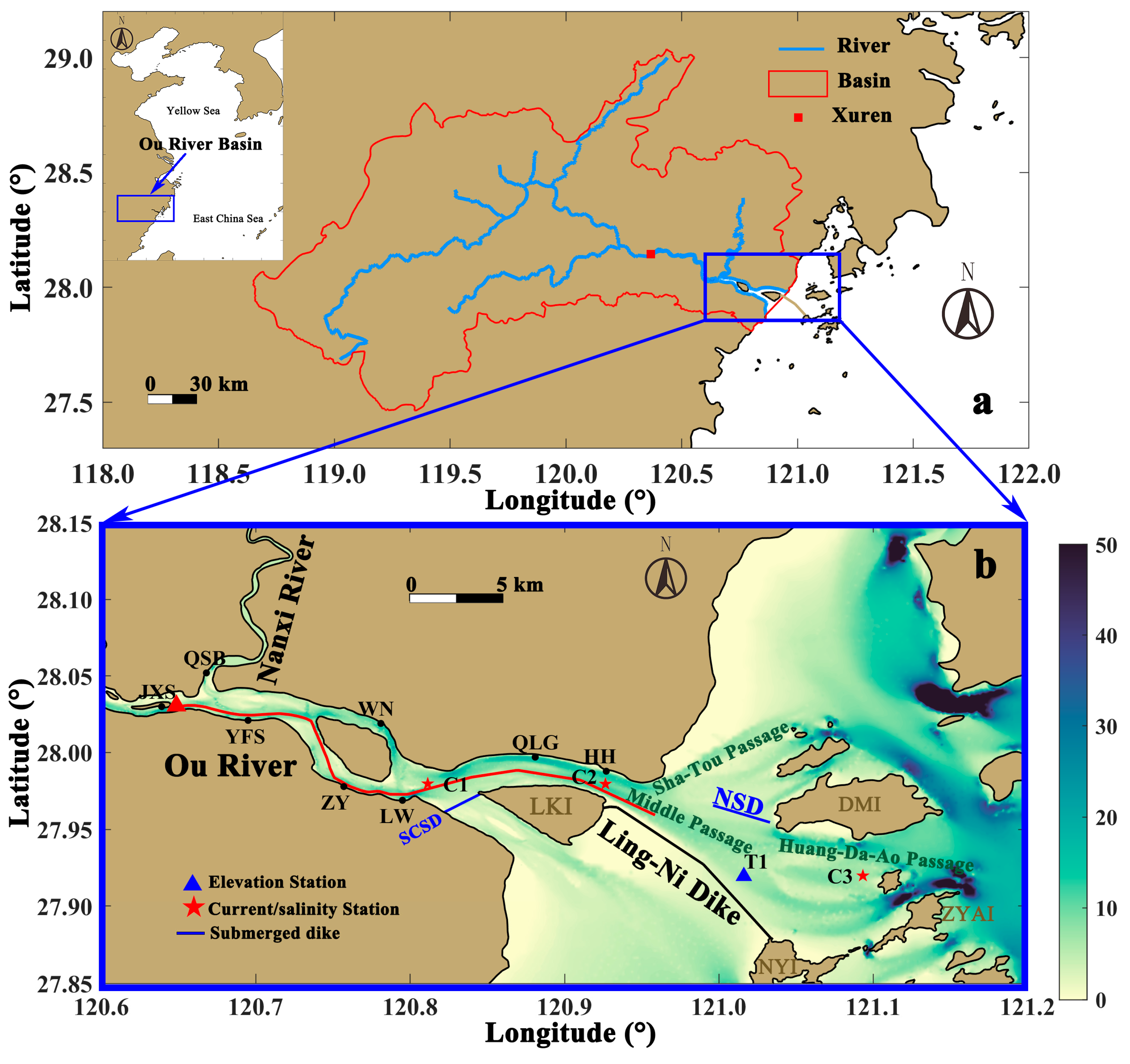
2.1. Study Area

The Ou River flows 388 km to the East China Sea, mainly through the Huang-Da-Ao Passage (Figure 1b). The Ou River discharge varies quickly in a short time during the plum-rainy/typhoon season, and the annual discharge of the river is 13.9 km³ [33]. The Ou River basin drains an area of ~1.80 × 10⁴ km², and the headwater comes from a mountain with peak elevation of 1856.7 m in the southwest Zhejiang Province [34]. Most of the rainfall is concentrated in plum-rainy/typhoon season (April to September), and annual precipitation varies from 1100 to 2200 mm [35]. The river runoff in plum-rainy/typhoon season accounts for 78% of the annual total [36]. The Ou River Estuary (ORE) is tide-dominated, and the largest tidal range and the smallest tidal range are 7.21 m and 1.14 m at the Huang-Hua tidal station (HH in Figure 1), respectively, indicating a macrotidal regime [37].

The ORE is split into the North and South Channels by Ling-Kun Island. To meet the demand of land use by socioeconomic development, a submerged dike (South Channel Submerged Dike) was built in 1979 in the South Channel to silt the South Channel and naturally and gradually form land. The North Channel, as a main channel, is further divided into the northeastward Sha-Tou Passage and the Middle Passage; it stretches along the North Submerged Dike, Ling-Ni Dike, and several islands, including Da-Men Island, Ni-Yu Island and Zhuang-Yuan-Ao Island (see Figure 1b for details).

2.2. Model Configuration

The hydrodynamic model and configuration used here is the same as that in the first part of this study [32], which is based on a three-dimensional unstructured grid primitive equation Finite-Volume Community Ocean Model (FVCOM) [38,39]. Considering a three-dimensional domain, the horizontal Reynolds-averaged momentum equation ignoring surface forcing after hydrostatic approximation [38] is given as follows:

$$\frac{\partial u}{\partial t}+u\frac{\partial u}{\partial x}+v\frac{\partial u}{\partial y}+w\frac{\partial u}{\partial z}-fv=\frac{\partial Pt}{\partial x}+\frac{\partial Pc}{\partial x}+\frac{\partial }{\partial z}\left(K_m\frac{\partial u}{\partial z}\right)+F_u$$

(1)

$$\frac{\partial v}{\partial t}+u\frac{\partial v}{\partial x}+v\frac{\partial v}{\partial y}+w\frac{\partial v}{\partial z}+fu=\frac{\partial Pt}{\partial y}+\frac{\partial Pc}{\partial y}+\frac{\partial }{\partial z}\left(K_m\frac{\partial v}{\partial z}\right)+F_v$$

(2)

where t is the time, x, y, and z are the east, north, and vertical axes in Cartesian coordinate system, (u, v, w) is the three-dimensional Cartesian velocity vector, f is the Coriolis parameter; Pt is the barotropic pressure, and Pc is the baroclinic pressure; K_m is the vertical eddy viscosity coefficient; F_u and F_v represent the horizontal momentum diffusion terms. The bottom boundary conditions for u and v are:

$$K_v\left(\frac{\partial u}{\partial z},\frac{\partial v}{\partial z}\right)=\frac{1}{\rho }\left({\tau }_{\mathrm{bx}},{\tau }_{by}\right)$$

(3)

where $\left({\tau }_{\mathrm{bx}},{\tau }_{by}\right)=C_d\sqrt{u^2+v^2}\left(u,v\right)$ are the x and y components of bottom stresses. The bottom friction coefficient C_d affected by SSC is showed in Equation (5).

To understand sediment trapping in estuaries, the SSC dynamics in the water column ignoring horizontal diffusion are described in [40,41]:

$$\frac{\partial C}{\partial t}+\frac{\partial \left(uC\right)}{\partial x}+\frac{\partial \left(vC\right)}{\partial y}+\frac{\partial \left[\left(w-w_s\right)C\right]}{\partial z}-\frac{\partial }{\partial z}\left(K_v\frac{\partial C}{\partial z}\right)=0$$

(4)

where $C\left(x,y,z,t\right)$ is the suspended sediment dry mass per water volume (grams per liter or kilograms per cubic meter), w_s is the suspended sediment settling velocity, and K_v is the eddy diffusivity for SSC. The vertical coordinate z ranges from the surface elevation $\eta (x,y,t)$ to bottom topography—$H(x,y,t)$.

In high-turbidity systems, sediment trapping can be enhanced by the suppression of turbulence due to turbidity-induced stratification in the bottom boundary layer [17,42]. As a result, Wang [43] applied the flux Richardson number R_f, which is an index of the vertical density stratification using the Mellor-Yamada Level 2.5 Turbulence Closure model, into the bottom friction coefficient to reproduce these effects into a numerical model:

$$C_{\mathrm{d}}={\left[\frac{\mathsf{\kappa }}{(1+\mathrm{A}{R}_f)\ln (z_b/z_{0b})}\right]}^2$$

(5)

where κ is the von Kármán constant, z_b is the near-bottom layer thickness, z_0b is the bottom roughness, and A = 5.5 is an empirical constant. According to Mellor and Yamada [44], the flux Richardson number R_f can be calculated as:

$$R_f=0.725\left[R_i+0.186-{\left(R_i{}^2-0.316R_i+0.0346\right)}^{1/2}\right]$$

(6)

where the gradient Richardson number (R_i) can be calculated as:

$$R_i=-\frac{g}{\rho }\frac{\partial \rho /\partial z}{{\left(\partial u/\partial z\right)}^2+{\left(\partial v/\partial z\right)}^2}$$

(7)

On the other hand, to quantitatively couple sediment transport with hydrodynamic, the equation of state using a bulk-density relation is represented as follows:

$$\rho ={\rho }_w+\left(1-\frac{{\rho }_w}{{\rho }_s}\right)\times C$$

(8)

where ρ_w is the seawater density, and ρ_s is the porosity sediment bulk density.

Vanished sediment flux at the free surface is required:

$$K_v\frac{\partial C}{\partial z}-C{w}_s=0 \mathrm{for} z=\eta .$$

(9)

The net sediment flux (E_b) normal to the bottom is the difference between the deposition and erosion, yielding

$$K_v\frac{\partial C}{\partial z}-C{w}_s=E_b \mathrm{for} z=-H$$

(10)

assuming small surface and bottom slopes. The well-accepted Ariathurai and Krone formulation [45] for E_b is:

$$E_b=\{\begin{array}{l}{E}_0\left(\frac{\left|{\tau }_b\right|}{{\tau }_{ce}}-1\right) \mathrm{if} \left|{\tau }_b\right|\ge {\tau }_{ce} \mathrm{Erosion}\hfill \\ C_b{w}_s\left(1-\frac{\left|{\tau }_b\right|}{{\tau }_{cd}}\right) \mathrm{if} \left|{\tau }_b\right|<{\tau }_{cd} \mathrm{Deposition}\hfill \end{array}$$

(11)

where E₀ is the constant erosion rate parameter, C_b is the SSC close to the bottom, τ_b is the bottom shear stress, and τ_ce and τ_cd are the critical shear stress for erosion and deposition, respectively.

Sediment settling is an essential process in estuarine sediment trapping [3]. For fine particles and high SSC, the cohesiveness of sediments becomes noteworthy; the settling velocity depends on the SSC and the turbulence intensity capturing processes. As a result, a general expression [46] for the settling velocity including physical processes such as free settling, flocculated settling, and hindered settling is

$$w_s=\{\begin{array}{ll}{w}_{s0}\hfill & C\le C_0\hfill \\ \frac{m_1{C}^{n_1}}{{\left(C^2+m_2{}^2\right)}^{n_2}}\hfill & C>C_0\hfill \end{array}$$

(12)

where w_s0 is the free settling velocity, C₀ is the critical concentration for flocculation, and m₁, m₂, n₁, and n₂ are empirical settling coefficients. The validated parameters in the suspended sediment model are summarized in

Table 1. Parameters used in the suspended sediment transport model.

Parameter	Value	Reference
τce	0.6 (kg·m−1·s−2)	Tested
τcd	0.6 (kg·m−1·s−2)	Tested
E0	5 × 10−5 (kg·m−2·s−1)	Tested
ws0	−2.11 × 10−5 (m·s−1)	Tested
m1	−0.05	Tested
n1	1.2	Mehta and McAnally [46]
m2	6.2	Mehta and McAnally [46]
n2	1.6	Mehta and McAnally [46]
C0	0.2 (kg·m−3)	Mehta and McAnally [46]
ρs	1100 (kg·m−3)	Tested
z0b	2.5 × 10−4 (m)	Tested

.

The model has a higher horizontal resolution (about 100 m) in the North Channel and Middle Passage (Figure 2) with 18 sigma layers in the vertical. FVCOM is implemented using a mode-split approach for computation efficiency, in which the three-dimensional momentum, salinity and SSC are integrated with internal mode time step (2 s) and sea elevation, defined as external mode, is integrated with a shorter time step (1 s). Different from the first part [32], the model was run starting on 9 December 2006, as we do not have the measured SSC data in 2005 for validation. In this part, the model was initiated with zero water level and velocity and was first run for 120 days with a fixed river discharge, including both OR and NR (the daily average on 8 April 2007) as well as the open boundary salinity (the monthly average in April 2007), to reach a quasi-equilibrium state. Due to the lack of observed river input SSC, the multiyear average of the river SSC during the plum-rainy/typhoon season (0.2 kg·m⁻³) was set in the model [33]. The model was then run with the daily average river discharge for another 45 days, from 8 April to 22 May in 2007, and the results from the last 35 days were analyzed. The wind wave was nonsignificant in the ORE due to the shelter effect of the island [47] and thus was not considered in this study. This case was marked as the Control Run (Run 0).

2.3. Validation

Fieldwork was carried out in the ORE from 23 April to 22 May 2007 (day of the year 113~142). Tidal elevation at a short-term tidal gauge (shown as T1 in Figure 1b) was recorded hourly by Temperature-Depth (Compact-TD) over the entire observation. Meanwhile, electromagnetic-current-meters and Conductivity-Temperature-Depths (CTDs) were used to record the current velocity and salinity during the neap tide from 11:00 24 April to 12:00 25 April (UTC +0800, day of the year 114.46~115.50) and the spring tide from 11:00 1 May to 12:00 2 May 2007 (UTC +0800, day of the year 121.46~122.50), with one-hour intervals at C1~C3 stations (shown in Figure 1b).

To validate the numerical model, the RSR, which is the ratio of the root mean square error (RMSE) normalized by the standard deviation of the observation [48] is used, which is calculated as:

$$RSR=\frac{\sqrt{{{\displaystyle \sum \left(X_{observation}-X_{model}\right)}}^2}}{\sqrt{{\displaystyle \sum {\left(X_{observation}-{\overline{X}}_{observation}\right)}^2}}}.$$

(13)

The Nash-Sutcliffe efficiency (NSE) is also used to validate the model, which is given as:

$$NSE=1-\frac{\sqrt{{{\displaystyle \sum \left(X_{observation}-X_{model}\right)}}^2}}{\sqrt{{\displaystyle \sum {\left(X_{observation}-{\overline{X}}_{observation}\right)}^2}}}.$$

(14)

X is the variable being evaluated; and the overbar indicates the temporal average. Comparison between the observed and simulated tidal elevation at T1 is shown in Figure 3. Referring to the performance ratings (

Table 2. General performance ratings [49].

Performance Rating	RSR	NSE	PBIAS (%) for Sediment
Very Good	0 ≤ RSR ≤ 0.50	0.75 ≤ NSE ≤ 1	PBIAS < ±15
Good	0.50 < RSR ≤ 0.60	0.65 ≤ NSE < 0.75	±15 < PBIAS < ±30
Satisfactory	0.60 < RSR ≤ 0.70	0.50 ≤ NSE < 0.65	±30 < PBIAS < ±55
Unsatisfactory	RSR > 0.70	NSE < 0.50	PBIAS > ±55

) in previous study [49], both RSR (0.24) and NSE (0.94) of tidal elevation showed very good values. Comparisons between the observation and simulated current velocity/direction at C1~C3 are shown in Figure 4. The RSR and NSE for along-channel flow are given in

Table 3. RSR and NSE of flow and salinity, PBIAS of SSC at the C1~C3 stations.

Station	Flow				Salinity				SSC
	Neap		Spring		Neap		Spring		Neap	Spring
	RSR	NSE	RSR	NSE	RSR	NSE	RSR	NSE	PBIAS (%)	PBIAS (%)
C1	0.40	0.84	0.36	0.87	0.41	0.83	0.57	0.68	6.65	20.02
C2	0.22	0.95	0.28	0.92	0.17	0.97	0.54	0.71	11.30	24.04
C3	0.44	0.81	0.51	0.74	0.50	0.75	0.69	0.52	−47.36	−31.27

. Most RSRs are less 0.50, and NSEs are greater than 0.75, indicating very good values. Comparisons between the simulated and observed salinities are also shown in Figure 5, and their RSRs and NSEs are summarized in Table 3. Most RSRs are less 0.60, and most NSEs are over 0.65, indicating that the model could reproduce the salinity variation (Table 3). Comparison between the simulated and observed SSC are shown in Figure 6, which focus on the bottom SSC as ETMs are most significant near the bottom [3]. Percent bias (PBIAS) is used to validate the SSC, given as [49]:

$$PBIAS=\frac{{\displaystyle \sum \left(X_{observation}-X_{model}\right)\times 100}}{{\displaystyle \sum \left(X_{observation}\right)}}.$$

(15)

The performance rating of the PBIAS for sediment is listed in Table 2. PBIASs of SSC are concluded in Table 3, and all values reach a satisfactory level, indicating the model can reproduce suspended sediment dynamics. Note that the river SSC during flooding can rise an order compared to a low-discharge condition [33], so the lack of observed river SSC may be the reason that SSC simulations are comparatively inaccurate. Overall, this numerical model is able to describe the hydrodynamics and suspended sediment transport in the ORE.

2.4. Experimental Design

Based on the ORE model, several experiments are designed to study the response of the turbidity maximum to a rapid-change discharge, which are summarized in

Table 4. Experiment configuration and the SSC and location of the ETM core in the along-channel section (the red line in Figure 1b with the red triangle indicating 0 km).

Run	Peak Discharge (m3·s−1)	PRD Occurrence Time	PRD Duration (Day)	River SSC during PRD (kg·m−3)	ETM Core SSC (kg·m−3)	ETM Core Location (km)
Run 0	Real type	-	-	-	-	-
Run 1	500	-	-	0.2	1.61	16.07
Run 2	Real type	Neap Tide	3	0.2	0.56	25.36
Run 3	Real type	Spring Tide	3	0.2	1.41	20.20
Run 4	500	-	-	0	1.38	16.24
Run 5	5000	Spring Tide	2	0	1.16	26.74
Run 6	3500	Spring Tide	3	0	1.15	28.11
Run 7	2750	Spring Tide	4	0	1.16	26.54
Run 8	2500	Spring Tide	2	0	1.38	20.38
Run 9	7500	Spring Tide	2	0	1.07	28.11
Run 10	10,000	Spring Tide	2	0	1.01	30.71
Run 11	2500	Spring Tide	2	0.4	1.44	20.38
Run 12	5000	Spring Tide	2	0.4	1.24	26.74
Run 13	7500	Spring Tide	2	0.4	1.28	28.11
Run 14	10,000	Spring Tide	2	0.4	1.23	30.71

. Taking the year 2007 as an example, a PRD with a peak discharge over 1000 m³·s⁻¹ occurred nine times and the maximum discharge reached 7310 m³·s⁻¹, which is approximately one order greater than the multiyear average value (442 m³·s⁻¹ by Song et al., [33]). A PRD event with a 1590 m³·s⁻¹ peak discharge (return period is about 13 years) was captured during field measurements (from 25 to 27 April, day of the year 113~142, Figure 7a). The daily average river discharge from 2005 to 2015 at the Xuren hydrologic station (Figure 1a) shows that the duration of a PRD event is usually less than 2 days in the ORE. Thus, the flooding duration is set to 2 days in some experiments. In contrast to Run 0, wind and NR are ignored in the other cases to focus on the Ou River PRD. Run 1 represents the low-discharge condition of a constant 500 m³·s⁻¹ (the solid blue line in Figure 7b), according to the multiyear average value of 442 m³·s⁻¹ [33]. Runs 2 and 3 are experiments in which the 3-day PRD measured during the observational period (Figure 7a) is given during neap tide and spring tide, respectively (Table 4). Run 4 is the same as Run 1 except that the river SSC is set to 0. The river SSC during PRD is set to 0 in Runs 5~10. Runs 5~7 have the same total river discharge volume during PRD but with different duration. Runs 8~10 have the same PRD duration (2 days) as Run 5, but have a different peak discharge. According to the daily average OR discharge collected from 2005 to 2015, the maximum discharge was 10,900 m³·s⁻¹, which was recorded in August 2014. Therefore, in Runs 8, 5, 9, and 10, the peak discharge is set to increase from 2500 m³·s⁻¹ (return period is about 30 years) to 10,000 m³·s⁻¹ (return period is about 3500 years) during spring tide with 2500 m³·s⁻¹ intervals to examine the impact of discharge volume on the ETM. Runs 11~14 use the same PRD duration (2 days) as Run 5, but have a different peak discharge and the river SSC during PRD is set to 0.4 kg·m⁻³.

3. Results

3.1. Saltwater Intrusion

3.1.1. Spring-Neap Modulation

The distribution of the salinity during spring and neap tides at the bottom layer of the ORE under the low-discharge condition is shown in Figure 8a–d. The saltwater at the bottom layer is more easily extended landward than at the surface [1]. Therefore, this section shows the location of the salt-wedge by the salinity at the bottom layer. The tidal cycle selected during the spring and neap tides is the last tidal cycle during the flooding. At high water slack, the salt-wedge of the ORE is closer to the Jiang-Xin-Si during spring tide than during neap tide. At high water slack, the salinity isoline of 1 PSU is mainly in the area of Yang-Fu-Shan to Zhuang-Yuan or Wu-Niu during the spring and neap tides, while the salinity isolines of 2 to 5 PSU during the neap tide are more intensive than during the spring tide (Figure 8a,b). At low water slack, as the main channel of runoff, the area of Yang-Fu-Shan to Zhuang-Yuan to Long-Wan is generally covered with freshwater during neap tide, and the salinity isoline of 5 PSU is located near Qi-Li-Gang (Figure 8c). During spring tide, the salt-wedge shifts to the east of the Qi-Li-Gang; at this moment, west of the Qi-Li-Gang, only part of the deeper areas keeps some saltwater with salinity of about 1 PSU (Figure 8d).

During both spring and neap tides, PRD moves the salt-wedge seaward (Figure 8e–h). At high water slack, during the neap tide, in the runoff main channel of Yang-Fu-Shan to Zhuang-Yuan to Long-Wan, the 1 PSU isoline shifts between Zhuang-Yuan and Long-Wan (Figure 8e). At high water slack, during the spring tide, the salt-wedge is more landward than the neap tide, and the head of the 1 PSU salinity isoline is about 1.2 km west of the Zhuang-Yuan (Figure 8f). Since the branch of Yang-Fu-Shan to Wu-Niu is not the main channel of runoff, the change of salt-wedge location is not obvious whether there is PRD or not (Figure 8f). At low water slack, the PRD pushes the salt-wedge downstream to the sea, and the salinity value near the Qi-Li-Gang is about 2 to 3 PSU during neap tide (Figure 8g). At the low water slack, under the PRD, 1 PSU salinity isoline is pushed near the Huang-Hua, except for areas with high water depth during spring tide (Figure 8h).

3.1.2. Stratification

Dyer [50] proposes a method for calculating the stratification intensity and classifying the mixing type called the stratification index, which is calculated by dividing the difference between surface and bottom salinity $\Delta S$ by the vertically averaged seawater salinity $\overline{S}$. According to Dyer [50], when the stratification index is less than 0.15, it is well-mixed; the indicator is partially mixed when between 0.15 and 0.32, and stratified when greater than 0.32. Figure 9 shows a distribution of the tidally averaged stratification index on the along-channel section during spring and neap tides. The along-channel section selects the position with the largest along-channel flow velocity, while the section also covers the area where the ETM may occur. Under the low-discharge condition, since the spring tide amplitude is stronger than the neap tide, the stratification during the spring tide is obviously weaker than during the neap tide. During neap tide, the stratification index is always greater than 0.32 (solid blue line in Figure 9) seaward from 16.4 km, indicating that the water is stratified. During spring tide, the stratification index is mostly lower than 0.32 and sometimes even lower than 0.15 (dashed blue line in Figure 9), indicating that the water has changed from stratified during neap tide to partially mixed or even mixed during spring tide.

Under the PRD, the tidally averaged stratification decreases from the landward head to 21.7 km during neap tide (the red solid line compared to the blue solid line in Figure 9) and to 20.9 km during spring tide (the red dashed line compared to the blue dashed line in Figure 9), but the PRD cannot alter the mixing type. This is because the PRD pushes the salt-wedge seaward, the position where it has a significant stratification at the head of the salt-wedge under the low-discharge condition, but is mostly covered with well-mixed freshwater under the PRD and becomes mixed. In these areas where the stratification index increases, the maximum stratification index rises from 0.76 (solid blue line in Figure 9) to 0.97 during the neap tide (solid red line in Figure 9), and the maximum stratification index rises from 0.37 (dashed blue line in Figure 9) to 0.42 during the spring tide (dashed red line in Figure 9).

3.2. Estuarine Turbidity Maximum

3.2.1. Spring-Neap Modulation

The distribution of the tidally averaged SSC during spring and neap tides at the bottom of the ORE is shown in Figure 10a–d. Since the most significant part of the ETM is located at the bottom, the location of the ETM is better reflected by the bottom SSC. Under the low-discharge condition, the ETM at the ORE is mainly located between the Yang-Fu-Shan and Long-Wan, with the core area located near Long-Wan, which is consistent with previous observations [51]. The stratification inhibits the vertical diffusion and therefore contributes to the SSC trapping. However, although the stratification during neap tide is larger than that during spring tide, the resuspended sediment caused by the tidal current decreases during neap tide, leading to a smaller core SSC of the ETM. During neap tide, the maximum SSC at the bottom of the ETM is 0.77 kg·m⁻³ (Figure 10a), while during spring tide, it can reach 1.61 kg·m⁻³ (Figure 10b). Under the PRD, the ETM shifts seaward during the spring and neap tides, and the SSC of the ETM core is reduced compared to the low-discharge condition, as the large amount of water carried by the PRD dilutes the ETM. During neap tide, the area enclosed by the 0.55 kg·m⁻³ SSC isoline under the PRD is significantly reduced compared to the low-discharge condition (red lines in Figure 10a,c); the core location also shifts downstream from the near Long-Wan (Figure 10a) to near Qi-Li-Gang (Figure 10c) by PRD. During spring tide, the area enclosed by the 1.35 kg·m⁻³ SSC isoline is significantly reduced under the PRD than under the low-discharge condition (red lines in Figure 10b,d), and the core location of the ETM shifts about 6 km downstream by the PRD (Figure 10b,d).

Figure 11 shows the tidally averaged SSC (filled contour and red isolines) and the tidally averaged salinity (blue isolines) on the along-channel section during the spring and neap tides, as well as the residual flow along the section. The residual flow is calculated by a moving average through a time window of a lunar day. During neap tide, under the low-discharge condition, the ETM is located 15~20 km, mainly near the 2~4 PSU salinity isolines (Figure 11a). Figure 11b shows the vertical structure of the residual flow, the upper-layer water with less salinity or smaller density is mainly seaward, and the lower-layer seaward runoff coverages with landward density-driven flow to form a stagnation point with zero residual flow velocity. The location of the ETM is near the position of the stagnation point. Under the PRD, both the locations of the ETM and the salt-wedge shift towards the sea, and the core location of the ETM shifts about 8 km downstream (Figure 11c). The location of the ETM is approximately the same as that of the 5~7 PSU salinity isolines, while the stagnation point also shifts downstream near the ETM (Figure 11c,d).

The location of the ETM during spring tide is similar to that during neap tide under the low-discharge condition, which is approximately the same as the position of the 1~2 PSU salinity isolines (Figure 11e). The stagnation point during spring tide is about 8 km downstream from the position during neap tide, and this seaward movement is due to the weaker stratification during spring tide compared with neap tide and the weakening of saltwater intrusion (Figure 11f). Under the PRD, during spring tide, the core ETM shifts about 5 km towards the sea, roughly near the 1~2 PSU salinity isolines position (Figure 11g). Meanwhile, the stagnation point is about 2 km downstream compared to the low-discharge condition, roughly at the head of the 3 PSU salinity isoline (Figure 11h). It is noteworthy that there is a relatively large SSC belt (with a maximum SSC of 0.44 kg·m⁻³) near the upstream part of the section (0~8 km) under the PRD during neap tide (Figure 11c). The formation of this belt is mainly because the PRD inputs a high amount of sediment in a short time into the channel, while the upstream water sediment transport is too weak to immediately move it downstream, resulting in the temporary suspended sediment storage (Figure 11c). However, under the PRD, during spring tide, such characteristics are not significant (Figure 11g) because the river SSC experiment design does not take into account that the river SSC increases during PRD [33] in Run 3, and SSC during spring tide is higher than neap tide. As a result, the temporary suspended sediment storage is not obvious during spring tide. This will be further discussed in Section 4.2.

3.2.2. Sediment Transport

The mean SSC flux through a unit-width cross section can be calculated as

$$T0=\frac{1}{T}{\displaystyle {\int }_0^T{\displaystyle {\int }_0^{h}Ucdzdt}}$$

(16)

where T is one or more tidal cycles, U is the horizontal flow vector, c is the SSC, h is the depth of water which changes with the tide level, and z is the vertical coordinate depth (0 for the bottom; h for the surface).

Uncles and Jordan [52] suggested that the factors in Equation (16) can be decomposed into

$$h=h_0+h_t$$

(17)

$$U=\overline{U_0}+\overline{U_t}+U^{\prime }$$

(18)

$$c=\overline{c_0}+\overline{c_t}+c^{\prime }$$

(19)

where the subscript “0” represents the tidally averaged value, the subscript “t” denotes the deviations from the tidally averaged value, a bar denotes a depth-mean value, and a prime denotes the deviations from the depth-mean value. Thus, Equation (16) can be rewritten as

$$T0=\underset{\mathrm{T}1}{\underbrace{h_0\overline{U_0}\overline{c_0}}}+\underset{\mathrm{T}2}{\underbrace{\overline{c_0}\langle h_t\overline{U_t}\rangle }}+\underset{\mathrm{T}3}{\underbrace{\langle h\overline{U_t}\overline{c_t}\rangle +\overline{U_t}\langle h_t\overline{c_t}\rangle }}+\underset{\mathrm{T}4}{\underbrace{\langle h\overline{U^{\prime }{c}^{\prime }}\rangle }}$$

(20)

where T0 is the net sediment transport, T1 represents the Eulerian transport, the tidally averaged SSC transport by the Eulerian residual flow, and T2 represents the Stokes-drift transport. T3 represents the coupling between the SSC and the hydrodynamics, which changes with the tide. This is because the phase of water depth, flow, and SSC are not fully orthogonal with the changes of tide, i.e., the tidal pumping effect. T4 represents the transport of SSC caused by coupling between the vertical shear of the flow and the vertical difference of the SSC. T1 and T2 are together known as Lagrangian transport.

During both spring and neap tides, the sediment transport is mainly controlled by the Eulerian transport and the Stokes-drift transport. Figure 12 shows the mean suspended sediment flux through a unit-width along the section. Under the low-discharge condition, during neap tide, sediment transport is generally seaward from the landward head to 26 km, while on the remaining part of the section, sediment transport is mostly landward, together forming a convergence area of sediment transport around 26 km (red line in Figure 12a). The sediment transport T0 magnitude is 0~0.67 kg·s⁻¹·m⁻¹, and the Eulerian transport T1 magnitude is 0~0.77 kg·s⁻¹·m⁻¹, which is the largest component. In addition, the T2 magnitude is 0.03~0.12 kg·s⁻¹·m⁻¹, the T3 magnitude is 0~0.08 kg·s⁻¹·m⁻¹, and the T4 magnitude is 0~0.04 kg·s⁻¹·m⁻¹ (Figure 12a). Similar to neap tide, sediment transport converges around approximately 23 km during spring tide (Figure 12b). During spring tide, the sediment transport T0 magnitude is 0~3.34 kg·s⁻¹·m⁻¹, and the Eulerian transport T1 magnitude is 0~3.62 kg·s⁻¹·m⁻¹, which is also the largest part of the magnitude. In addition, the T2 magnitude is 0.22~0.80 kg·s⁻¹·m⁻¹, the T3 magnitude is 0~0.48 kg·s⁻¹·m⁻¹, and the T4 magnitude is 0~0.13 kg·s⁻¹·m⁻¹ (Figure 12b). During both the spring and neap tides, the convergence area of sediment transport is generally downstream from the position of the ETM and stagnation point (Figure 11). Because Equation (16) calculates the vertical averaged sediment transport, and the largest part of the SSC in the ETM is near the bottom, the area of the vertical averaged sediment transport convergence and the ETM position will not be accurately consistent. Additionally, Stokes-drift transport is always landward. The landward sediment transport during spring tide (seaward from 23 km) is mainly attributed to Stokes-drift transport (Figure 12b).

In general, the PRD drives the Eulerian transport (T1) seaward, and by contrast, the changes of the remaining terms are not significant, so the pattern of the main control sediment transport mechanism remains the same (Figure 12). For example, under the PRD, the magnitude of T0 is 0~1.50 kg·s⁻¹·m⁻¹ during neap tide, and the magnitude of T0 is 0~3.76 kg·s⁻¹·m⁻¹ during spring tide (Figure 12c,d). It is noteworthy that the maximum net sediment transport during neap tide under the PRD is 0~8 km on the along-channel section, which is different from that under the low-discharge condition (Figure 12c). Considering the temporary suspended sediment storage (Figure 11e), on the along-channel section at 0~8 km, the PRD increases the average sediment transport from 0.40 kg·s⁻¹·m⁻¹ under the low-discharge condition to 0.91 kg·s⁻¹·m⁻¹. Meanwhile, it more easily transports the stored suspended sediment downstream (Figure 12c).

4. Discussion

4.1. Sediment Source to Form ETM

The suspended sediment from river discharge cannot affect the location of ETM. Results (Section 3, Figure 11) indicate that ETMs are in similar positions and have similar response characteristics to PRD during neap and spring tides. However, the ETM is stronger in spring tide and is thus discussed further. Figure 13 shows a tidally averaged SSC distribution with the same total amount of PRD but under different PRD durations and under a low-discharge condition, without taking into account the river SSC. Under the low-discharge condition, when the river is no longer supplying sediment, the ETM position (Figure 13a) is similar to when the river is supplying sediment (Run 1, Figure 11e), located at approximately 15~20 km of the section. However, the SSC of the ETM without river suspended sediment supply is lower than that with river suspended sediment supply. Taking the ETM core as an example, the SSC at the core with river suspended sediment supply (Run 1) can reach 1.55 kg·m⁻³ (Figure 11a), while the SSC of the ETM core without river suspended sediment supply (Run 4) decreases to 1.38 kg·m⁻³ (Figure 13a). It indicates the sediment source of ETM in the Ou River is mainly derived from the resuspension of the seabed.

The large amount of water brought by the PRD has two effects on ETM: (1) the water brought by the PRD into the sea dilutes the ETM; (2) that water can change the water velocity and then change the bottom shear stress, such that the seabed may provide more suspended sediment into the water. Taking a peak discharge of the PRD with 5000 m³·s⁻¹ (return period is about 170 years) as an example, while the PRD pushes both the ETM and salt-wedge seaward, the SSC of the ETM core is reduced to 1.16 kg·m⁻³ (Run 5, Figure 13b) compared with that under the low-discharge condition (Run 4, Figure 13a). Figure 14 shows the bottom shear stress, and the net sediment flux E_b which represents the SSC flux of the seabed, under the low-discharge condition (Run 4) and the PRD condition (Run 5) without river suspended sediment supply during the PRD. PRD decreases both the bottom shear stress and the net sediment flux E_b during flood tide and increases them during ebb tide (Figure 14). During the 2-day PRD, the average net sediment flux of Run 5 is 4.84 × 10⁻⁵ kg·m⁻²·s⁻¹ (Figure 14d) on the along-channel section, which increases compared with that under the low-discharge condition (Run 4, Figure 14b) of 4.52 × 10⁻⁵ kg·m⁻²·s⁻¹, indicating that the seabed resuspends more SSC to the water during the PRD. This has also been observed in Delaware River Estuary, Trenton, New Jersey, USA, by Sommerfield and Wong [53] that during a PRD the seabed can be eroded more severe, which can last for several tidal cycles. The white dashed lines in Figure 14 indicate the ETM location under the low-discharge condition. The strongest seabed resuspension area, providing the largest SSC into water, is not located where the ETM develops (Figure 14). This suggests that the SSC resuspended from seabed needs to be transported by the estuarine circulation to develop the ETM. The difference in bottom shear stress caused by different PRDs is another factor affecting the ETM. Generally, when the PRD peak discharge is smaller, the ETM is more landward. When the total volume of PRD is the same, the duration is longer, and the peak discharge is smaller. The total amount of PRD in Figure 13c,d is equal to that in Figure 13b; meanwhile, the PRD in Run 6 lasts for 3 days (Figure 13c) and the PRD in Run 7 lasts for 4 days (Figure 13d). Taking the SSC isolines of 0.6~1.0 kg·m⁻³ in Figure 13b–d as indicators, the ETM becomes more landward as peak discharge decreases. Meanwhile, the SSC at the core of the ETM varies according to different PRD durations. The SSC at the core of the ETM during 3-day PRD (Run 6, Figure 13c) is slightly lower than that during 2-day PRD (Run 5, Figure 13b) and 4-day PRD (Run 7, Figure 13d), but with a difference of less than 0.02 kg m⁻³.

4.2. ETM Recovery Time

PRD imports a high amount of suspended sediment in a short time and the upstream water sediment transport is too weak to move it seaward in time. As a result, the sediment brought by the PRD is temporarily stored in the upstream channel. Subsequently, this sediment can be transported downstream by estuarine circulation. Figure 15 shows the recovery of the stored suspended sediment in the channel with PRD with a river SSC of 0.4 kg·m⁻³ and a peak discharge of 5000 m³·s⁻¹ (Run 12). Since the river SSC is set to the multiyear plum-rainy/typhoon season average, it is difficult to distinguish the stored suspended sediment in the channel during the spring tide with PRD (Run 3, Figure 11g). Previous work [33] on the river SSC of the Ou River during flooding shows that the river SSC during PRD can be an order greater than the average. Therefore, despite the lack of river SSC measurement during PRD, in the experiment design, it is reasonable to set the river SSC during PRD as twice the multiyear plum-rainy/typhoon season average. The distribution of tidally averaged SSC during PRD with enhanced river SSC is shown in Figure 15a. Compared to the 5000 m³·s⁻¹ peak discharge PRD without river suspended sediment supply (Run 5, Figure 13b), the SSC of the ETM core with river suspended sediment supply (Run 12, Figure 15a) is higher, and the location is closer to the location of the ETM under the low-discharge condition (Run 1, Figure 11e). Additionally, sediment storage occurs at 0~5 km of the along-channel section in Run 12 (Figure 15a), but does not occur in Run 5 without river suspended sediment supply (Figure 13b), which has the same PRD volume as Run 12, indicating that the sediment storage is due to the river suspended sediment supply. One day after the PRD, the stored suspended sediment near the section landward side is gradually transported downstream, and the ETM and salt-wedge move upstream by the density-driven flow (Figure 15b). The stored suspended sediment and the ETM converge at the location of the ETM under the low-discharge condition, at which moment, the SSC of the ETM core is still smaller than that under the low-discharge condition (Figure 11e) but in the same order (2 days after the PRD, Figure 15c). Subsequently, the SSC of the ETM core gradually increases to the value under the low-discharge condition and eventually recovers to normal. For example, in Run 12, the SSC of the ETM core 3 days after the PRD is close to the SSC under the low-discharge condition (Figure 15d).

In Equation (14), the NSE, which is closer to 1, the precision of the simulation is higher, is used to evaluate the ETM recovery including both position and magnitude. When the observation value X_obs and the simulation value X_model in Equation (14) are replaced by the tidally averaged SSC value on each vertical layer under the low-discharge condition and the PRD, respectively, the NSE indicates a measure for the recovery of the ETM from the disturbed state by the PRD to the low-discharge condition. When the NSE calculated after the PRD is close enough to 1, the ETM affected by the PRD is considered to have recovered to the low-discharge condition. To determine the effect of river suspended sediment supply on recovery time, Figure 16a shows the NSE after the different peak discharge PRDs (2-day duration) without river suspended sediment supply (Runs 5 and 8~10); Figure 16b is similar to Figure 16a, but the PRD has river suspended sediment supply (Runs 11~14). Comparisons of these experimental results show that whether the river suspended sediment supply or not, the NSE affected by PRD initially decreases from 1 and then gradually increases after the end of the PRD (Figure 16). The NSE increases slowly after it reaches 0.90, so 0.90 is taken as the threshold to determine whether or not the ETM recovers to a low-discharge condition (Figure 16).

Table 5. Recovery time (unit: hour) of the ETM after PRD with peak discharge (unit: m³·s⁻¹) shown in the parentheses.

River SSC during PRD (kg·m−3)	Run 8 (2500)	Run 5 (5000)	Run 9 (7500)	Run 10 (10,000)
0	111.8	138.7	142.7	142.8
River SSC during PRD (kg·m−3)	Run 11 (2500)	Run 12 (5000)	Run 13 (7500)	Run 14 (10,000)
0.4	85.0	94.7	97.3	110.7

shows the ETM recovery time after different peak discharge PRDs, with and without river suspended sediment supply. Under the river without suspended sediment supply, the recovery time of the ETM is 111.8~142.8 h after the 2500~10,000 m³·s⁻¹ peak discharge PRDs. Generally, the larger the peak discharge is, the longer the recovery time will be. However, the recovery time increases slowly after the peak discharge reaches a threshold. For example, the recovery times of Run 9 and Run 10 are similar (Table 5). The river can supply the sediment to the diluted ETM and reduce the recovery time. Under the river with suspended sediment supply, the recovery time of the ETM is 85.0~110.7 h after the 2500~10,000 m³·s⁻¹ peak discharge PRDs. Meanwhile, the recovery time with river suspended sediment supply is shorter than that without river suspended sediment supply (Table 5). Figure 16b shows that NSE has a larger fluctuation during the PRD (0~48 h) than that after the end of PRD, except for Run 11 due to the small peak discharge. This suggests that the suspended sediment supplied by PRD contributes to the increase of NSE to 1 or a reduction in the recovery time of the ETM. In addition, previous studies also found that the spring-neap modulation [31] and the antecedent discharge conditions [30] may affect the ETM recovery time through affecting the salinity distribution.

5. Conclusions

Small/medium-sized rivers are more likely to have PRDs during the plum-rainy/typhoon season, which becomes important to study its impact on the hydrodynamic and sediment dynamics as the global warming-induced inundation risks rise and terrestrial sediment sequestration increases. Based on some in-situ measurements including tidal elevation, tidal current, salinity, and SSC, the numerical model of the ORE is validated.

Under the low-discharge condition, the stratification during spring tide is obviously weaker than that during neap tide, and the PRD generally makes the stratification stronger. During spring tide, the turbidity maximum in the ORE is larger than that during neap tide. Although stronger stratification during neap tide would facilitate sediment trapping, the stronger tidal current during spring tide resuspended more sediment than that during neap tide. In addition, the positions of the ETM during spring tide and neap tide are similar. While the PRD pushes the ETM downstream, it also dilutes the ETM by bringing a large amount of water.

Based on the mechanism decomposition of sediment transport, during both neap and spring tides, the sediment transport is mostly induced by Eulerian transport and Stokes-drift transport. Generally, the PRD drives an additional seaward Eulerian transport seaward, and by contrast, the changes of the remaining terms are not significant and the pattern of the main control sediment transport mechanism remains unchanged. As a result, the ETM in the ORE is generally induced by residual current, or the sediment convergence of the seaward river flow and landward density-driven flow.

The sediment source of the ETM in the ORE is mainly derived from the sediment resuspension from the seabed. The PRD changes the bottom shear stress, so that the seabed can provide more suspended sediment into the water.

In addition, the suspended sediment brought by the PRD contributes to the recovery of the diluted ETM after the PRD, or the ETM affected by the PRD can recover to a low-discharge condition more quickly. The suspended sediment brought by the PRD will be temporarily stored in the upstream channel, because the upstream water sediment transport is too weak to move it downstream in time. Subsequently, this stored sediment can be transported downstream by estuarine circulation.

With river suspended sediment supply, the recovery times are 85.0~110.7 h under PRDs with a peak discharge of 2500~10,000 m³·s⁻¹, and the larger the peak discharge is, the longer the recovery time will be. Since the vertical mixing during neap tide is weaker than that during spring tide, we speculate that the ETM recovery time to PRD is slightly longer than that during spring tide. The morphological evolution of small/medium-sized river estuaries due to extreme weather conditions is not yet sufficiently understood. Therefore, the impact of the PRD on the morphological evolution, the transport, and the fate of the Ou River’s watershed suspended particulate matter in the ORE or the East China Sea will be further explored.

References

1. Geyer, W.R.; MacCready, P. The estuarine circulation. Annu. Rev. Fluid Mech. 2014, 46, 175–197. [Google Scholar] [CrossRef]
2. Maccready, P.; Geyer, W.R. Advances in estuarine physics. Annu. Rev. Mar. Sci. 2012, 2, 35–58. [Google Scholar] [CrossRef] [PubMed] [Green Version]
3. Burchard, H.; Schuttelaars, H.M.; Ralston, D.K. Sediment Trapping in Estuaries. Annu. Rev. Mar. Sci. 2018, 10, 371–395. [Google Scholar] [CrossRef] [PubMed]
4. Milliman, J.D. Sediment discharge to the ocean from small mountainous rivers: The New Guinea example. Geo Mar. Lett. 1995, 15, 127–133. [Google Scholar] [CrossRef]
5. Hibma, A.; Schuttelaars, H.M.; de Vriend, H.J. Initial formation and long-term evolution of channel-shoal patterns. Cont. Shelf Res. 2004, 24, 1637–1650. [Google Scholar] [CrossRef]
6. Xie, D.; Pan, C.; Gao, S.; Wang, Z.B. Morphodynamics of the Qiantang Estuary, China: Controls of river flood events and tidal bores. Mar. Geol. 2018, 406, 27–33. [Google Scholar] [CrossRef]
7. Olabarrieta, M.; Geyer, W.R.; Coco, G.; Friedrichs, C.T.; Cao, Z. Effects of density-driven flows on the long-term morphodynamic evolution of funnel-shaped estuaries. J. Geophys. Res. Earth 2018, 123, 2901–2924. [Google Scholar] [CrossRef] [Green Version]
8. Rodrigues, M.; Fortunato, A.B.; Freire, P. Saltwater intrusion in the upper Tagus Estuary during droughts. Geosciences 2019, 9, 400. [Google Scholar] [CrossRef] [Green Version]
9. Weng, X.; Jiang, C.; Zhang, M.; Yuan, M.; Zeng, T. Numeric Study on the Influence of Sluice-Gate Operation on Salinity, Nutrients and Organisms in the Jiaojiang River Estuary, China. Water 2020, 12, 2026. [Google Scholar] [CrossRef]
10. Hirabayashi, Y.; Mahendran, R.; Koirala, S.; Konoshima, L.; Yamazaki, D.; Watanabe, S.; Kim, H.; Kanae, S. Global flood risk under climate change. Nat. Clim. Chang. 2013, 3, 816–821. [Google Scholar] [CrossRef]
11. Schubel, J.R. Turbidity maximum of the northern Chesapeake Bay. Science 1968, 161, 1013–1015. [Google Scholar] [CrossRef] [PubMed] [Green Version]
12. Meade, R.H. Landward transport of bottom sediments in estuaries of the Atlantic coastal plain. J. Sediment Res. 1969, 39, 222–234. [Google Scholar]
13. Song, D.; Wang, X.H.; Kiss, A.E.; Bao, X. The contribution to tidal asymmetry by different combinations of tidal constituents. J. Geophys. Res. Oceans 2011, 116, C12007. [Google Scholar] [CrossRef]
14. Uncles, R.J.; Elliott, R.C.A.; Weston, S.A. Dispersion of salt and suspended sediment in a partly mixed estuary. Estuaries 1985, 8, 256–269. [Google Scholar] [CrossRef]
15. Postma, H. Transport and accumulation of suspended matter in the Dutch Wadden Sea. Neth. J. Sea Res. 1961, 1, 148–190. [Google Scholar] [CrossRef]
16. Jay, D.A.; Musiak, J.D. Particle trapping in estuarine tidal flows. J. Geophys. Res. Oceans 1994, 99, 20445–20461. [Google Scholar] [CrossRef]
17. Geyer, W.R. The importance of suppression of turbulence by stratification on the estuarine turbidity maximum. Estuaries 1993, 16, 113–125. [Google Scholar] [CrossRef]
18. Bartholdy, J. Processes controlling import of fine-grained sediment to tidal areas: A simulation model. In Coastal and Estuarine Environments: Sedimentology, Geomorphology and Geoarchaeology; Pye, K., Allen, J.R.L., Eds.; Special Publications of the Geological Society: London, UK, 2000; Volume 175, pp. 13–29. [Google Scholar]
19. Burchard, H.; Flöser, G.; Staneva, J.V.; Badewien, T.H.; Riethmüller, R. Impact of density gradients on net sediment transport into the Wadden Sea. J. Phys. Oceanogr. 2008, 38, 566–587. [Google Scholar] [CrossRef] [Green Version]
20. Scully, M.E.; Friedrichs, C.T. Sediment pumping by tidal asymmetry in a partially mixed estuary. J. Geophys. Res. Oceans 2007, 112, C07028. [Google Scholar] [CrossRef] [Green Version]
21. Winterwerp, J.C. Fine sediment transport by tidal asymmetry in the high-concentrated Ems River: Indications for a regime shift in response to channel deepening. Ocean Dyn. 2011, 61, 203–215. [Google Scholar] [CrossRef] [Green Version]
22. Ralston, D.K.; Geyer, W.R.; Warner, J.C. Bathymetric controls on sediment transport in the Hudson River estuary: Lateral asymmetry and frontal trapping. J. Geophys. Res. Oceans 2012, 117, C10013. [Google Scholar] [CrossRef] [Green Version]
23. Hudson, A.S.; Talke, S.A.; Jay, D.A. Using satellite observations to characterize the response of estuarine turbidity maxima to external forcing. Estuar. Coast. 2017, 40, 343–358. [Google Scholar] [CrossRef]
24. Fugate, D.C.; Friedrichs, C.T.; Sanford, L.P. Lateral dynamics and associated transport of sediment in the upper reaches of a partially mixed estuary, Chesapeake Bay, USA. Cont. Shelf Res. 2007, 27, 679–698. [Google Scholar] [CrossRef]
25. McSweeney, J.M.; Chant, R.J.; Sommerfield, C.K. Lateral variability of sediment transport in the Delaware Estuary. J. Geophys. Res. Oceans 2016, 121, 725–744. [Google Scholar] [CrossRef] [Green Version]
26. Le Hir, P.; Ficht, A.; Jacinto, R.S.; Lesueur, P.; Dupont, J.-P.; Lafite, R.; Brenon, I.; Thouvenin, B.; Cugier, P. Fine sediment transport and accumulations at the mouth of the Seine estuary (France). Estuaries 2001, 24, 950–963. [Google Scholar] [CrossRef]
27. Traykovski, P.; Geyer, R.; Sommerfield, C. Rapid sediment deposition and fine-scale strata formation in the Hudson estuary. J. Geophys. Res. Earth 2004, 109, F02004. [Google Scholar] [CrossRef] [Green Version]
28. Mitchell, S.; Akesson, L.; Uncles, R. Observations of turbidity in the Thames Estuary, United Kingdom. Water Environ. J. 2012, 26, 511–520. [Google Scholar] [CrossRef]
29. Song, D.; Wang, X.H.; Cao, Z.; Guan, W. Suspended sediment transport in the Deepwater Navigation Channel, Yangtze River Estuary, China, in the dry season 2009: 1. Observations over spring and neap tidal cycles. J. Geophys. Res. Oceans 2013, 118, 5555–5567. [Google Scholar] [CrossRef]
30. Sanford, L.P.; Suttles, S.E.; Halka, J.P. Reconsidering the physics of the Chesapeake Bay estuarine turbidity maximum. Estuaries 2001, 24, 655–669. [Google Scholar] [CrossRef]
31. Ralston, D.K.; Geyer, W.R. Episodic and long-term sediment transport capacity in the Hudson River estuary. Estuar. Coast. 2009, 32, 1130–1151. [Google Scholar] [CrossRef]
32. Yan, Y.; Song, D.; Bao, X.; Ding, Y. The Response of Lateral Flow to Peak River Discharge in a Macrotidal Estuary. Water 2020, 12, 3571. [Google Scholar] [CrossRef]
33. Song, L.; Xia, X.M.; Liu, Y.F.; Cai, T.L. Variations in water and sediment fluxes from Oujiang River to estuary. J. Sediment Res. 2012, 1, 46–52. (In Chinese) [Google Scholar]
34. Shang, S.; Fan, D.; Yin, P.; Burr, G.S.; Zhang, M.; Wang, Q. Late Quaternary environmental change in Oujiang delta along the northeastern Zhe-Min Uplift zone (Southeast China). Palaeogeogr. Palaeoclimatol. Palaeoecol. 2018, 492, 64–80. [Google Scholar] [CrossRef]
35. Zhang, M.Y.; Fan, D.D.; Wu, G.X.; Shang, S.; Chen, L.L. Palynological characters of late Quaternary in the South flank of the Oujiang River delta and their paleoclimate implications. Quat. Sci. 2012, 6, 182–195. (In Chinese) [Google Scholar]
36. Xie, Q.C.; Li, B.G.; Xia, X.M.; Li, Y.; Van Weering, T.C.E.; Berger, G.W. Spatial and temporal variations of tidal flat in the Oujiang estuary in China. Acta Geograph. Sin. 1994, 49, 509–516. (In Chinese) [Google Scholar]
37. Zuo, L.Q.; Lu, Y.; Li, H. Further study on back silting and regulation of mouth bar in Oujing estuary. Hydro Sci. Eng. 2012, 3, 6–13. (In Chinese) [Google Scholar]
38. Chen, C.; Liu, H.; Beardsley, R.C. An unstructured grid, finite-volume, three-dimensional, primitive equations ocean model: Application to coastal ocean and estuaries. J. Atmos. Ocean. Technol. 2003, 20, 159–186. [Google Scholar] [CrossRef]
39. Chen, C.; Beardsley, R.C.; Cowles, G. An Unstructured Grid, Finite-Volume Coastal Ocean Model (FVCOM) System. Oceanography 2006, 19, 78–89. [Google Scholar] [CrossRef] [Green Version]
40. Song, D.; Wang, X.H. Suspended sediment transport in the Deepwater Navigation Channel, Yangtze River Estuary, China, in the dry season 2009: 2. Numerical simulations. J. Geophys. Res. Oceans 2013, 118, 5568–5590. [Google Scholar] [CrossRef]
41. Kumar, M.; Schuttelaars, H.M.; Roos, P.C. Three-dimensional semi-idealized model for estuarine turbidity maxima in tidally dominated estuaries. Ocean Model. 2017, 113, 1–21. [Google Scholar] [CrossRef]
42. Wang, X.H.; Byun, D.; Wang, X.; Cho, Y. Modelling tidal currents in a sediment stratified idealized estuary. Cont. Shelf Res. 2005, 25, 655–665. [Google Scholar] [CrossRef]
43. Wang, X.H. Tide-induced sediment resuspension and the bottom boundary layer in an idealized estuary with a muddy bed. J. Phys. Oceanogr. 2002, 32, 3113–3131. [Google Scholar] [CrossRef]
44. Mellor, G.L.; Yamada, T. A Hierarchy of Turbulence Closure Models for Planetary Boundary Layers. J. Atmos. Sci. 1974, 31, 1791–1806. [Google Scholar] [CrossRef] [Green Version]
45. Ariathurai, R.; Krone, R.B. Finite element model for cohesive sediment transport. J. Hydr. Eng. Div. 1976, 102, 323–338. [Google Scholar]
46. Mehta, A.J.; McAnally, W.H. Fine-grained sediment transport. In Sedimentation Engineering: Processes, Measurements, Modeling, and Practice; Garcia, M.H., Ed.; American Society of Civil Engineers: New York, NY, USA, 2008; pp. 253–306. [Google Scholar]
47. Yao, S.; Li, S.; Liu, H.; Lu, Y.; Zhang, C. Experiment study on effects of waterway regulation structures on flood capacity of river. Port Waterw. Eng. 2010, 6, 120–126. (In Chinese) [Google Scholar]
48. Passerotti, G.; Massazza, G.; Pezzoli, A.; Bigi, V.; Zsoter, E.; Rosso, M. Hydrological Model Application in the Sirba River: Early Warning System and GloFAS Improvements. Water 2020, 12, 620. [Google Scholar] [CrossRef] [Green Version]
49. Moriasi, D.N.; Arnold, J.G.; Van Liew, M.W.; Bingner, R.L.; Harmel, R.D.; Veith, T.L. Model evaluation guidelines for systematic quantification of accuracy in watershed simulations. Trans. ASABE 2007, 50, 885–900. [Google Scholar] [CrossRef]
50. Dyer, K.R. Estuaries: A Physical Introduction, 2nd ed.; Wiley: London, UK, 1997; p. 195. [Google Scholar]
51. Zhang, X.; Chen, X.; Dou, X.; Zhao, X.; Xia, W.; Jiao, J.; Xu, H. Study on formation mechanism of turbidity maximum zone and numerical simulations in the macro tidal estuaries. Adv. Water Sci. 2019, 30, 86–94. (In Chinese) [Google Scholar]
52. Uncles, R.J.; Jordan, M.B. Residual fluxes of water and salt at two stations in the Severn Estuary. Estuar. Coast. Mar. Sci. 1979, 9, 287–302. [Google Scholar] [CrossRef]
53. Sommerfield, C.K.; Wong, K.C. Mechanisms of sediment flux and turbidity maintenance in the Delaware Estuary. J. Geophys. Res. 2011, 116, C01005. [Google Scholar] [CrossRef]
Figure 1. (a) The Ou River Basin with the Xuren hydrologic station. (b) Zoom-in of the blue box in (a); bathymetry of the ORE (color, unit: m). The red line is the along-channel section used in this study. LKI: Ling-Kun Island; DMI: Da-Men Island, NYI: Ni-Yu Island; ZYAI: Zhuang-Yuan-Ao Island; NSD: North Submerged Dike; SCSD: South Channel Submerged Dike; JXS: Jiang-Xin-Si; QSB: Qing-Shui-Bu; ZY: Zhuang-Yuan; WN: Wu-Niu; LW: Long-Wan; QLG: Qi-li-Gang; HH: Huang-Hua.
Water 13 00106 g001
Figure 2. Mesh grid of the ORE model used in this study. Red curve indicates open boundary.
Water 13 00106 g002
Figure 3. Observed (dot red line) and simulated (solid blue line) tidal elevation at the T1 station.
Water 13 00106 g003
Figure 4. Observed (dot red line) and simulated (solid blue line) vertical averaged current velocity and current direction during neap tide (ac current velocity in m·s−1; df current direction in degree) and spring tide (gi current velocity in m·s−1; jl current direction in degree) at the C1~C3 stations.
Water 13 00106 g004
Figure 5. Observed (dot red line) and simulated (solid blue line) vertical averaged salinity (PSU) during (ac) neap tide and (df) spring tide at the C1~C3 stations.
Water 13 00106 g005
Figure 6. Observed (dot red line) and simulated (solid blue line) bottom suspended sediment concentration (kg·m−3) during (ac) neap tide and (df) spring tide at C1~C3 stations.
Water 13 00106 g006
Figure 7. (a) River discharge of the OR during the in-situ measurement. (b) Two types of river discharge (blue lines) in experiment runs: the solid line is for low-discharge, the dashed line with squares is for PRD.
Water 13 00106 g007
Figure 8. Distribution diagram of bottom salinity (filled contour, unit: PSU) under (ad) the low-discharge condition and (eh) PRD condition at high water slack and low water slack. The salinity is in 1-PSU intervals. Left panels are during neap tide, and right panels are during spring tide. White areas indicate tidal flat.
Water 13 00106 g008
Figure 9. Stratification index on the along-channel section (the red line in Figure 1b with the red triangle indicating 0 km) during neap tide (colored solid lines) and spring tide (colored dashed lines). Black dashed lines indicate the thresholds of 0.15 and 0.32, respectively.
Water 13 00106 g009
Figure 10. Distribution diagram of tidally averaged bottom SSC (filled contour, unit: kg·m−3) under (a,b) the low-discharge condition and (c,d) PRD condition. Upper panels are during neap tide, and lower panels are during spring tide. White areas indicate tidal flat.
Water 13 00106 g010
Figure 11. (left panels) Tidally averaged SSC (red lines and filled contour, unit: kg·m−3) and salinity (blue lines, unit: PSU) distribution on the along-channel section during neap tide (a,c) and during spring tide (e,g). The SSC is in 0.1 kg·m−3 intervals and the salinity is in 1-PSU intervals. (right panels) Along-channel residual flow velocity (filled contour, unit: m·s−1) distribution on the along-channel section during neap tide (b,d) and during spring tide (f,h). Positive indicates seaward.
Water 13 00106 g011
Figure 12. Tidally averaged SSC transport and its decomposed terms on the along-channel section under (a,b) the low-discharge condition and (c,d) PRD condition. Upper panels are during neap tide, and lower panels are during spring tide. Positive value means seaward transport.
Water 13 00106 g012
Figure 13. Tidally averaged SSC (red lines and filled contour, unit: kg·m−3) and salinity (blue lines, unit: PSU) distribution on the along-channel section during spring tide when river SSC is set to 0 under (a) the low-discharge condition, (b) a 2-day-PRD duration, (c) a 3-day-PRD duration and (d) a 4-day-PRD duration. The SSC is in 0.1 kg·m−3 intervals and the salinity is in 1-PSU intervals.
Water 13 00106 g013
Figure 14. Time series diagram of (left) bottom shear stress (filled contour, unit: N·m−2) and (right) net sediment flux (filled contour, unit: ×10−4 kg·m−2·s−1) on the along-channel section during spring tide when river SSC is set to 0 under (a,c) the low-discharge condition and (b,d) a 2-day PRD. White dashed lines indicate ETM location under the low-discharge condition. Shadows indicate flood tide.
Water 13 00106 g014
Figure 15. Tidally averaged SSC (red lines and filled contour, unit: kg·m−3) and salinity (blue lines, unit: PSU) distribution on the along-channel section during spring tide with the 5000 m3·s−1 peak discharge PRD when the river SSC is set to 0.4 kg·m−3 (Run 12), and the tidal cycle is (a) the last during PRD, (b) a day later than (a), (c) two days later than (a), and (d) three days later than (a). The SSC is in 0.1 kg·m−3 intervals, and the salinity is in 1-PSU intervals.
Water 13 00106 g015
Figure 16. Recovery times of the ETM indicated by the NSE when (a) the river SSC is set to 0 and (b) the river SSC is set to 0.4 kg·m−3. Dashed lines indicate 0.90. Note the vertical axis range differs.
Water 13 00106 g016