Uncertainty Evaluation in Hydrological Frequency Analysis Based on Confidence Interval and Prediction Interval

Abstract

The shortage of extreme rainfall data gives substantial uncertainty to design rainfalls and causes predictions for torrential rainfall to deviate strongly from adopted probability distributions used in river planning. These torrential rainfalls are treated as outliers which existing studies do not evaluate. However, probability limit method test which its acceptance region expresses with high accuracy the range where observed ith order statistics could realize. Confidence interval which quantifies uncertainty of adopted distributions can be constructed by assuming that these critical values in both sides of the adopted region follow the same function form applied to actual observed data. Furthermore, its validity is proved through comparison of confidence interval derived from ensemble downscaling calculations. In addition, these critical values are almost in accordance with outliers in samples from the ensemble downscaling calculations. Therefore, prediction interval which expresses the range that an unknown observed datum can take is constructed by extrapolating the critical values for limit estimation of a future datum. In this paper, quantification method of uncertainty of design rainfall and occurrence risk of outliers in the traditional framework, using the proposed confidence interval and prediction interval, is shown. Moreover, their application to future climate by using Bayesian statistics is explained.

1. Introduction

In traditional flood control management, probable rainfall is estimated by conducting statistical analysis of extreme rainfall data accumulated through rainfall observation over several decades. Extreme rainfall data can be divided into two types. An Annual Maximum Series is a statistical sample constructed of annual maximum rainfalls extracted from observed time series of rainfalls. A Peaks Over Threshold data set is a statistical sample constructed of extreme values exceeding a given threshold. Statistical analysis of such data is called hydrological frequency analysis [1]. The mathematical part of these hydrological frequency analysis methods is based on extreme value theory, whose basis was constructed by Fisher and Tippet [2]. They proved that the maximum values of any sample asymptotically approach one of three types of extreme value distribution. These three types of extreme value distribution are the Gumbel distribution, the Frechet distribution, and the negative Weibull distribution in the present. Gumbel [3] also adopted a type I maximum asymptotic distribution for expressing the probability distribution of flood discharge. This research of Gumbel’s pioneered hydrological frequency analysis in the context of extreme value theory. Later, Gnedenko [4] proved a necessary and sufficient condition in order for probability distributions to belong to a domain of attraction of extreme value distribution. In addition, von Mises [5] and Jenkinson [6] proposed a generalized extreme value distribution, which can express each of the three types of extreme value distribution noted above. Gumbel’s “Statistics of Extremes” [7] summarized the main research results of extreme value theory of that era. Coles [8] and de Haan [9] illustrated subsequent developments of extreme value theory. Based on this previous research, modern hydrological frequency analysis is conducted as follows. First, several probability distributions are selected as candidates for frequency analysis. Second, probability distributions selected as candidates in the first step are applied to extreme hydrological data such as extreme rainfall or extreme river discharge, and parameters of these probability distributions are estimated. Third, estimated probability distributions are evaluated in a comparative framework based on goodness-of-fit criteria and stability [10]. Through this procedure, a single probability distribution is adopted for frequency analysis. Finally, a T-year hydrological quantity is estimated based on the adopted probability distribution. Although this procedure is solidly established, statistical estimation in hydrological frequency analysis involves substantial uncertainty because the total number of observed extreme rainfall data are limited, ranging from about several tens to 200. This shortage of extreme rainfall data makes it difficult to evaluate torrential heavy rainfalls. 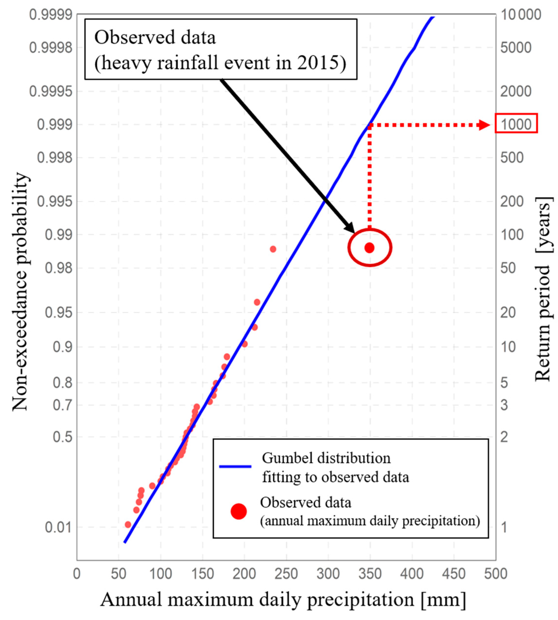Takara [11] pointed out that the observed data for torrential rainfalls deviate strongly from adopted probability distributions in river planning. In addition, the return period for these observed data calculated by the adopted probability distribution is thousands of years to tens of thousands of years, which can be orders of the magnitude longer than the observation data set length. For an example of this difficulty, Figure 1 shows observed data for the annual maximum daily rainfall for 36 years at Ikari observatory in the Tone river basin of Japan, along with a Gumbel distribution fitted to these observed data and an observed datum for a heavy rainfall event in 2015. Based on this figure, the observed datum of heavy rainfall event deviates strongly from the adopted Gumbel distribution, and the return period for this datum is 1000 years. Observed data with such a return period are often treated as outliers [12], because major river planning in Japan is designed based on hydrological values with return periods of about 100 to 200 years [11]. Design return periods in major river basins of various countries are shown in

Table 1. Design return periods in major river basins of various countries.

Country Name	Targeted River Basin	Planned Return Period
United States	Lower basin of Mississippi river	About 500 year
England	Thames river	1000 year (Tidal area including London)
The Netherlands	Primary flood defense	2000~10,000 year (Coastal area)
Japan	Ara river	200 year

[13,14,15,16,17,18]. These data make clear that each case of river planning involves difficulty in managing extreme hydrological events with return periods of several thousands of years, especially in Japan. Furthermore, the estimation error increases by extrapolation of the probability distribution when estimating probable hydrological quantities corresponding to long-term return periods exceeding the observation period. Especially, the flood control management of The Netherlands uses the traditional concept of return period, considering the effects of climate change and economic development as global warming proceeds [19]. Meanwhile, in recent years in Japan, rainfall events of heaviness exceeding recorded maximum have occurred frequently, causing severe damage to society. Therefore, it is necessary to formulate flood control management in the face of the intensification of heavy rainfall caused by climate change accompanied with global warming. Therefore, in this research, we propose evaluation method of uncertainty of design rainfall and prediction method for torrential rainfall. These methods are constructed by using the theory of probability limit method test [20] which can theoretically estimate the range where observed data could realize (acceptance region), including outliers in traditional hydrological frequency analysis. In addition, an application of these methods to future climate by incorporation of ensemble climate projection data using Markov Chain Monte Carlo method is shown in this paper.

In existing studies, to evaluate heavy rainfalls treated as outliers or record-breaking rainfall, occurrence probabilities of these rainfalls are often analyzed. For example, Itokawa et al. [21] calculated the distribution of the number of new records from each observatory in Japan and compared the derived distribution to the theoretical one, demonstrating a good accordance between the two distributions. Yamada et al. [22] investigated the number of annual maxima for daily and 3-day total precipitation measurements in Japan, discussing the effects of climate change. In addition, to manage torrential rainfall in future climate, a flood risk evaluation method using an ensemble climate projection database has been proposed to deal with the intensification of heavy rainfall accompanied by climate change [23,24,25,26]. An ensemble climate projection database contains numerous calculated results for meteorological values for past and future climate. Such database can be interpreted as rainfall data possibly experienced in the past and to be experienced in the future. Yamada et al. 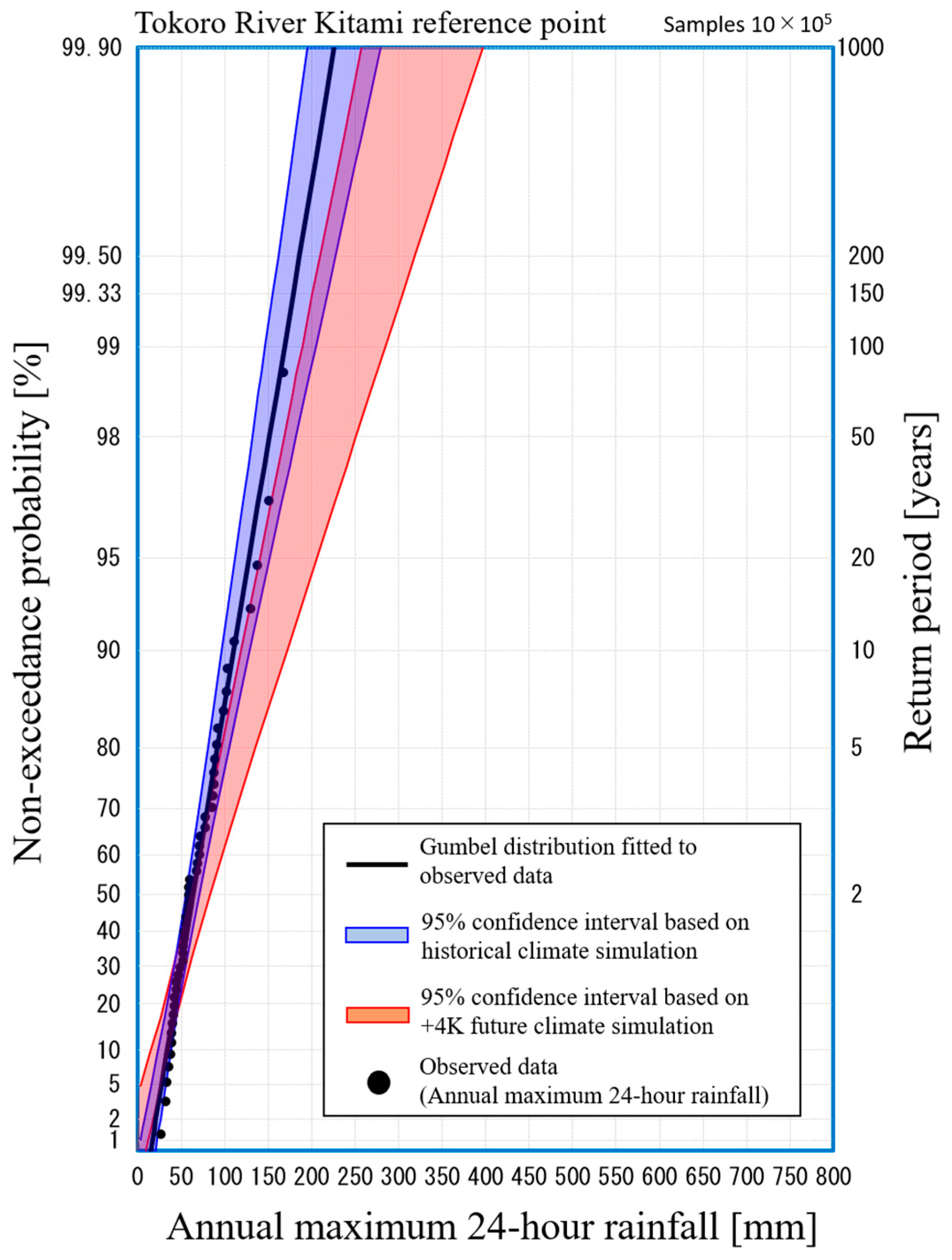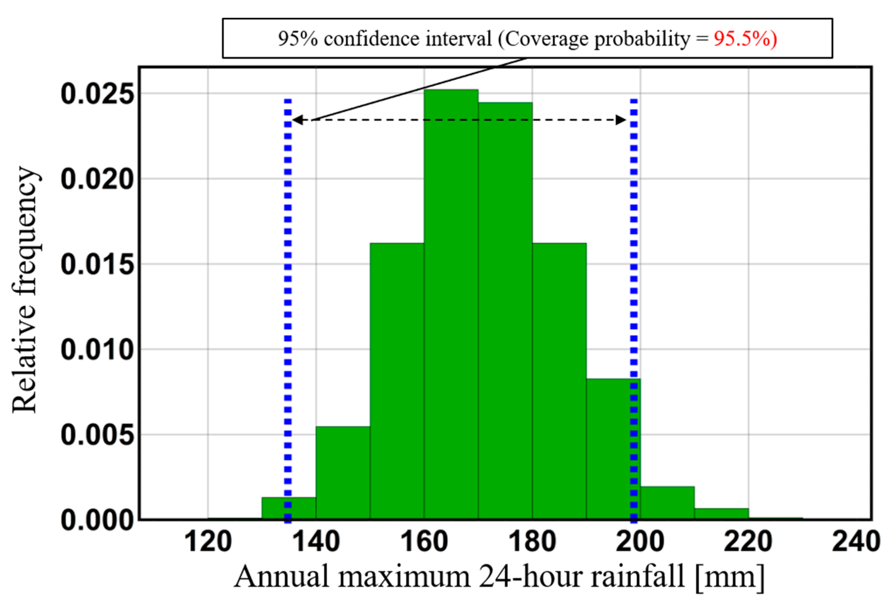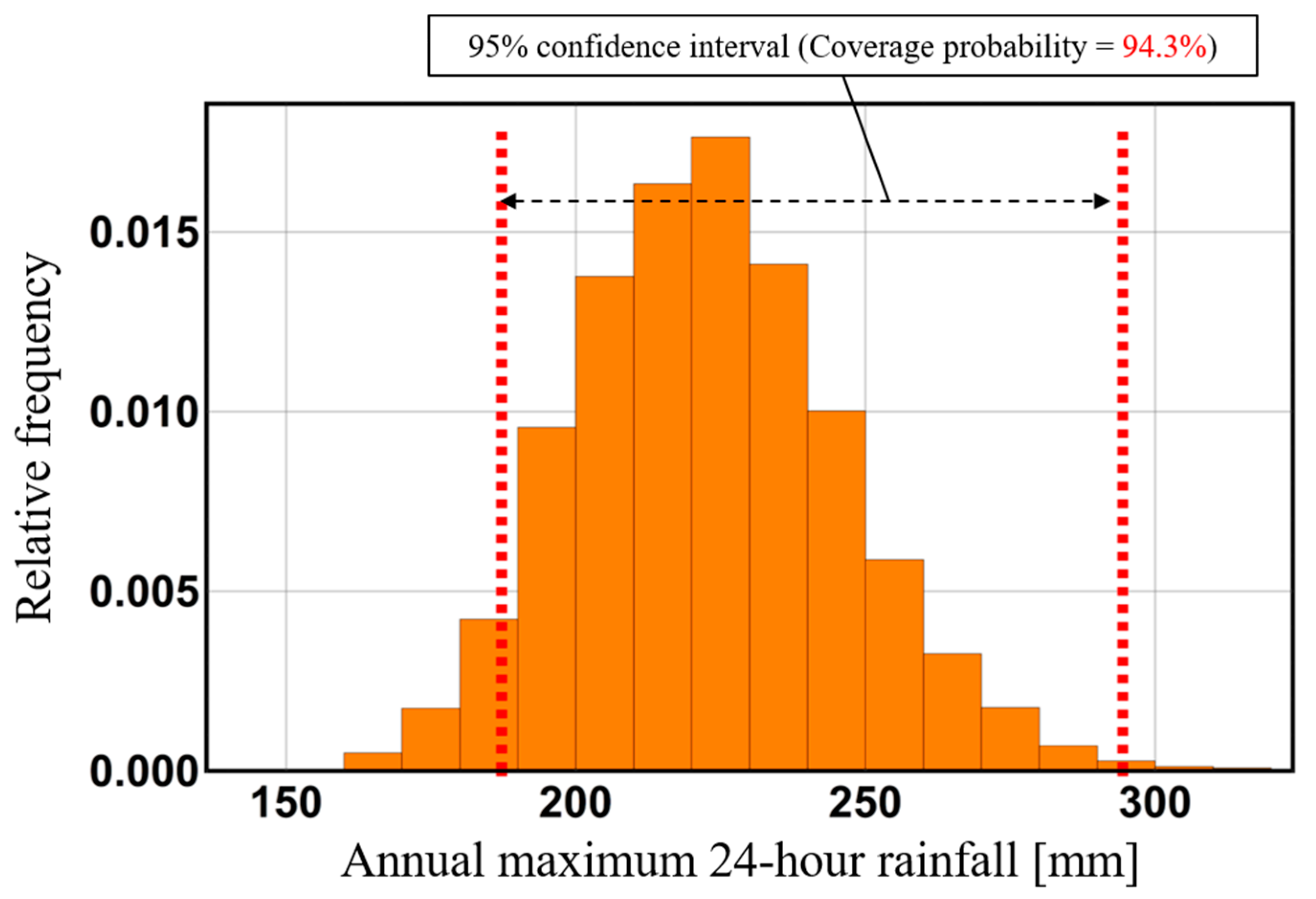[23,25,26] conducted downscale calculations of the ensemble climate projection database d4PDF and constructed a horizontal, high-resolution database of resolution high enough to evaluate future rainfall characteristics. Ensemble downscaling calculations makes it possible to intercorporate actual observed data and simulation data to compensate for the shortage of observed data when considering flood control management. In traditional flood control management, the design rainfall is decided using only a sample of the observed data available. On the other hand, this horizontal, high-resolution database allows for rational quantification of the design rainfall’s uncertainty caused by the shortage of observed data. The range of this design rainfall uncertainty is defined as a confidence interval. 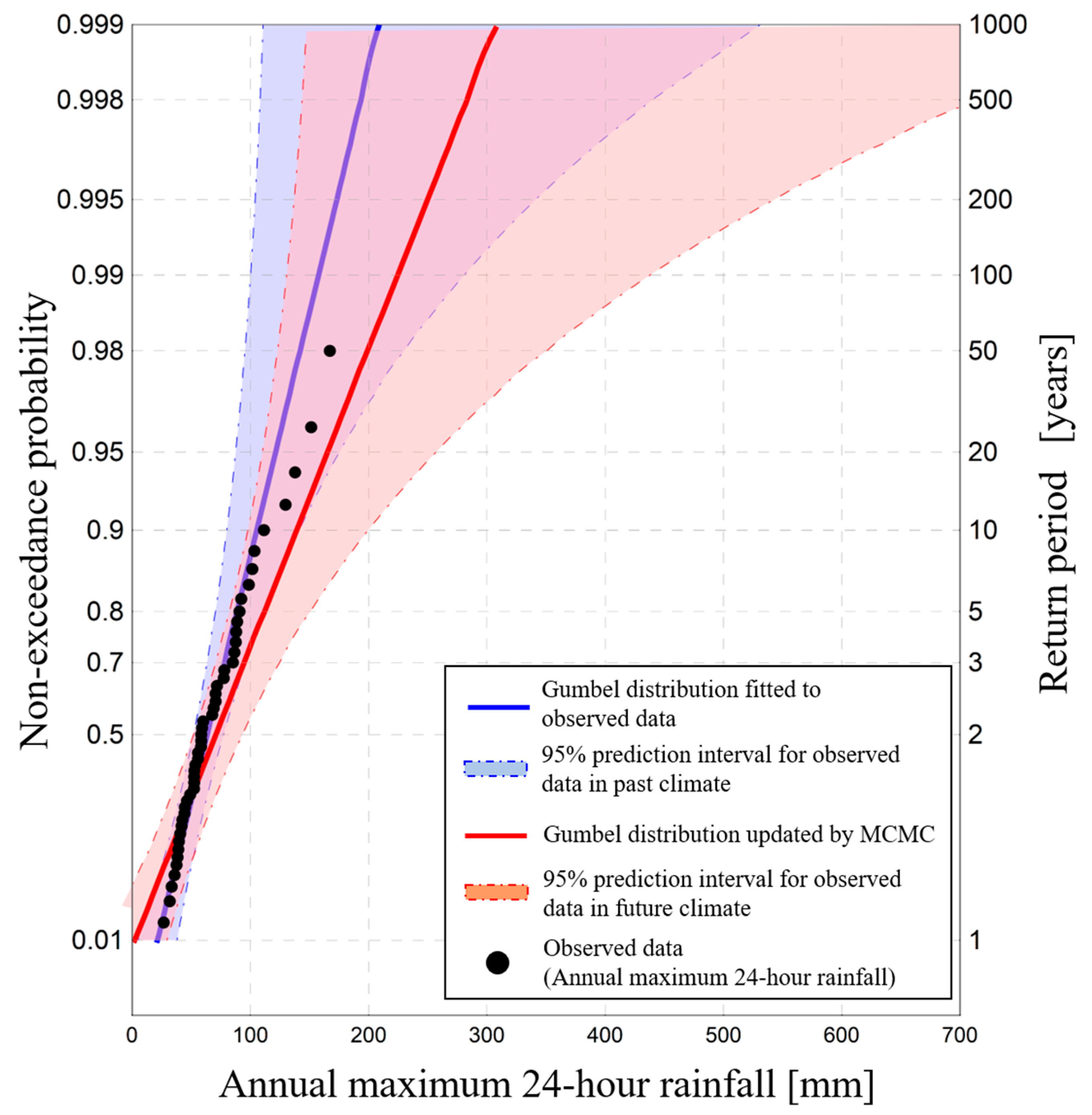As an example, Figure 2 shows observed data of annual maximum 24-h rainfall in the Tokoro river basin (black points), a Gumbel distribution fitted to the observed data (solid black line), a 95% confidence interval on past climate (blue range), and a 95% confidence interval on future climate in which average global temperature increases by 4K from the era of industrial revolution [23,25,26]. These confidence intervals can be derived from a physical Monte Carlo method using

Ensemble statistical samples from both the past and the +4K future of this horizontal, high-resolution database. In the field of conventional mathematical statistics or frequency analysis, confidence intervals are often expressed by numerical methods such as the jackknife or bootstrap method [27]. Many of these conventional methods use an assumption of normality based on the central limit theorem to estimate statistics. However, it can be difficult to treat a distribution of probable rainfall as a normal distribution. It can also be problematic to assume a normal distribution for T-year extreme rainfall given the limited extreme rainfall data available at present. Our proposed confidence interval does not use above mentioned assumptions. On the other, to handle unsteadiness caused by climate change, the nonstationary extreme value analysis is effective. Stationarity of rainfall is assumed in traditional hydrological frequency analysis but prevents consideration of unsteadiness caused by climate change [27]. Therefore, in general, probability distributions that dominate hydrological systems, such as rainfall, as modeled in traditional analysis, do not reflect real-world change. In nonstationary analysis method, nonstationary extreme value distribution model whose parameter is function of time is generally used. By this time-varying parameter, detecting of unsteadiness of natural phenomenon and expressing time variation of T-year extremes can be possible. However, increasing number of parameters concerning time might cause estimation error. Detailed explanation of theory and models in nonstational frequency analysis are shown by Coles [8] and Khaliq [28]. Recently, effectiveness of nonstationary analysis against climate change is shown in existing studies through derivation nonstational T-year annual monthly temperature [29] and future change of T-year annual maximum rainfall [30]. Moreover, large ensemble climate simulations enable estimation of design hydrological quantity by using thousands of samples to delete substantial uncertainty inherit estimated values. For example, Wiel et al. [31] simulates 2000 years by using global climate model and global hydrological model for a present-day and 2 K warmer climate in the Paris climate agreements [32] and evaluated T-year discharge by empirical distribution and stational extreme value distribution constructed of simulated discharges to quantify future change of T-year discharge. In addition, The Royal Netherlands Meteorological Institute [33] in the Netherlands has conducted future projection for flood discharge in Rhine river and estimated T-year discharge based on empirical distribution constructed of calculated discharge from large ensemble climate projections, according to global warming scenarios. Here, we assume there still exists uncertainty in estimation, because although ensemble climate projection data enable us to use thousands sample, initial conditions or boundary conditions are reflected on actual observed information. Therefore, it can be said that estimated values have uncertainty caused by finiteness of observed information. The frequency analysis based on probability limit method test we propose can express this kind of uncertainty as a form of acceptance region, for probability distribution constructed of a lot of data from ensemble climate projections. On the other hand, there is the effective concept of prediction interval which can evaluate observed data of torrential rainfall in future time. A prediction interval is defined as a range determined by observed data into which future data are expected to fall. Considering this definition, a prediction interval includes a distribution of a random variable expressing observed data for a future time with a given confidence coefficient. Many parts of the theoretical framework of prediction intervals are provided by Takeuchi [34]. On the other hand, little previous research has focused on prediction intervals for extreme values. In previous research, prediction intervals for extreme values have been constructed using the assumption of a normal distribution, a t-distribution, and so on, for extreme values. However, as Kitano [35] pointed out, it may be preferable to adopt extreme value distributions for probability distributions of extreme values, rather than a normal distribution or a t-distribution. Recently, a construction method for prediction intervals of extreme values was provided by Kitano [35]. The method proposed is superior to previous methods from the perspective that it does not need an assumption of normality. Coles [36] and Kitano [37] proposed construction methods for prediction distributions for extreme values by constructing a prior distribution for parameters of the extreme value distribution and applying a Markov Chain Monte Carlo method to update more rational prediction for extremes. In their research, outliers are considered as realized values in right tail of prediction distribution or interval. Based on this concept, prediction possibility of outliers is shown through prediction distribution or prediction interval constructed by MCMC which evaluates outliers in prior information by incorporation of each obtainment of newly observed data. Considering these previous studies, we newly incorporate ensemble climate projection data in MCMC method to make rational estimation for heavy rainfall in future climate.

For solution against uncertainty caused by finiteness of observed extreme rainfall data, prediction difficulty of torrential heavy rainfall in present and future situation, we used a probability limit method test [20] to construct a new hydrological frequency analysis based on confidence intervals and prediction interval that does not require any parametric assumptions as possible. The introduction of confidence intervals allows risk in flood control management to be expressed by considering where a given rainfall datum lies within the confidence interval. In addition, this research, based the construction methods for prediction intervals on the theory of the probability limit method test, provides a theoretical framework for the estimation of scale and occurrence risk of heavy rainfall in future. However, analysis based on confidence intervals and prediction intervals still requires an assumption of stationarity, meaning that the probability characteristics of hydrological events do not change as time proceeds. Therefore, confidence intervals and prediction intervals reflecting the effects of climate change can be constructed by incorporating information from future projection data into the updating of these intervals. This paper presents a method for deriving confidence intervals and prediction intervals under a situation of progressive global warming by incorporating climate projection data into extreme value distributions derived from past observed extreme rainfall data currently available. Based on this update of confidence interval and prediction interval, uncertainty of design rainfall and the magnitude of torrential rainfall itself in future climate is estimated.

The organization of this paper is as follows. Section 2 shows the mathematical theory of confidence interval and prediction interval. Section 3 shows the detail of probability limit method test and construction method of confidence interval and prediction interval based on this hypothesis test theory. Section 4 shows estimation methods to construct extreme value distribution in future climate, based on Markov Chain Monte Carlo method incorporating ensemble climate projection data. Section 5 shows the results of validity evaluation of confidence interval based on the theory of probability limit method test and the acceptance region of the theory through comparison of ensemble climate projection data. Section 6 summarizes the main results of this research.

2. Formulation of Confidence Interval and Prediction Interval

This section provides the method of statistical estimation and prediction. The concepts of confidence interval and prediction interval are also illustrated.

2.1. Method of Statistical Estimation

Statistical estimation is the estimation of characteristic values of populations based on an available sample X = {X₁, X₂, …, X_n}. Among statistical estimation methods are point estimation and interval estimation methods. Point estimation assigns parameter $\mathit{\theta }$ an estimated statistic $\widehat{\mathit{\theta }}$ derived from an available sample. On the other hand, interval estimation derives an interval constructed from a lower confidence limit value $L_{C.I.}\left(X\right)$and an upper confidence limit value $U_{C.I.}\left(X\right)$based on an available statistical sample. Interval estimation verifies that this interval includes true value of parameter with a probability of more than (1 − p), where p (0 < p < 1) is defined as a significance level. An interval [$L_{C.I.}\left(X\right)$, $U_{C.I.}\left(X\right)$] is defined as a 100(1 − p)% confidence interval for parameter $\mathit{\theta }$ as follows [38]:

$$P\left(L_{C.I.}\left(X\right)\le \mathit{\theta }\le U_{C.I.}\left(X\right)\right)\ge 1-p$$

(1)

where (1 − p) is a confidence coefficient.

We next illustrate in detail the definition and usage of confidence intervals for probability distributions. A confidence interval for a probability distribution D(X;$\widehat{\mathit{\theta }}$) is defined as follows. Here, X represents a random variable, $\mathit{\theta }$ expresses a parameter of the probability distribution of random variable X, and n expresses the total number of observations. The confidence interval of the probability distribution is then the range over which probability distributions fall when derived by fitting the same function to each of N ensemble samples and estimating the parameter, for N experiments or observations under the same conditions. Here, the sample size of each N-ensemble sample X ^j_ens. (where j = 1, 2…, N) is n, the same as the total number of observations. For example, a 95% confidence interval of probability distribution D(X;$\widehat{\mathit{\theta }}$) is the range on which about 95% of N probability distributions D(X;${\widehat{\mathit{\theta }}}^j$) (where j = 1, 2,…, N) fall. Here, j expresses the sample number, while F_X(x) expresses a cumulative density function of the probability distribution fitted to the observed data. The confidence interval for cumulative density function F_X(x) is shown in Equation (2).

$$P\left(L_{C.I.}\left(X\right)\le F_X\left(x\right)\le U_{C.I.}\left(X\right)\right)\ge 1-p$$

(2)

2.2. Method of Statistical Prediction

Statistical prediction predicts the future values of an unknown random variable Y. In hydrology, this method is used to predict extreme rainfall Y at a future time using past observed data X. Among statistical prediction methods are point prediction and interval prediction methods. Point prediction predicts future data Y by assigning one predicted value $\widehat{Y}$ derived from a sample X to an unknown random variable Y. On the other hand, interval prediction predicts by positing that future data exist with an arbitrary probability within an interval constructed from the lower prediction limit value $L_{P.I.}\left(X\right)$ and the upper prediction limit value $U_{P.I.}\left(X\right)$ derived from sample X. The prediction interval for future values of an unknown random variable Y is [34]

$$P\left(L_{P.I.}\left(X\right)\le Y\le U_{P.I.}\left(X\right)\right)\ge 1-p,$$

(3)

where interval [$L_{P.I.}\left(X\right)$, $U_{P.I.}\left(X\right)$] verifies that Y is included in this interval with a probability at least as great as (1 − p), called the 100(1 − p)% prediction interval. When estimating the range on which the adopted probability distribution derived from sample X falls, the confidence interval should be used. On the other hand, when prediction of future extremes themselves is needed, a prediction interval should instead be used.

3. Methodology

The probability limit method test [20] is a hypothesis test theory that improves the weak power of the Kolmogorov–Smirnov test [39,40] at the tail of an assumed probability distribution. In addition, Anderson–Daring test [41,42] gives more weight to the tails than does Kolmogorov–Smirnov test. Kolmogorov–Smirnov test is a nonparametric test in the sense that the distribution of test statistics is theoretically decided, without setting assumption of parametric distribution to test statistics. Anderson–Darling test makes use of the specific distribution in calculating critical values [43]. This has the advantage of allowing a more sensitive test and the disadvantage that critical values must be calculated for each distribution. In addition, probability limit method test has an advantage whose acceptance region can be constructed with no assumption of specific distribution concerning a variable in its region. The power of a test is the probability of rejecting a null hypothesis. The greater the power of the test of the adopted hypothesis, the narrower the confidence interval and prediction interval based on this test and the greater the accuracy of estimation and prediction. In the probability limit method test, a critical line of the probability limit method, called the probability limit line, is constructed on each side of an assumed probability representing function. Significant difference with the null hypothesis is found when observed data fall outside the interval defined by the limit lines. Here, the probability representing function is defined as the inverse function of the cumulative density function [44].

In the following, D(X;$\mathit{\theta }$) represents an assumed probability distribution, F_X(x) represents the cumulative density function of D(X;$\mathit{\theta }$), and χ_X(u) represents the probability representing function of D(X;$\mathit{\theta }$). As above, X represents a random variable, while random variable U (= F_X(x)) represents the cumulative probability of X. The forms of the cumulative density function (F_X(x)) and the probability representing function χ_X(u) are respectively shown in Equations (4) and (5).

$$u=F_X\left(x\right)$$

(4)

$$x={\chi }_X\left(u\right)$$

(5)

3.1. Kolmogorov–Smirnov Test

Kolmogorov [39] proposed a maximum difference between the “cumulative density function of an assumed distribution” and the “empirical cumulative density function” as test statistics. Smirnov [40] showed tables of realized values of the test statistics Kolmogorov proposed. Through these analyses, the theoretical framework of Kolmogorov–Smirnov test was developed. The Kolmogorov–Smirnov test is one of the hypothesis test theories for testing goodness-of-fit between an assumed cumulative density function F_X(x) and an observed sample X when a sample X (= {x₁,x₂,…, x_n}) is treated as an independent sample from an unknown population which has continuous cumulative density function F_T(x). In this context, null hypothesis H₀ and alternative hypothesis H₁ are described as follows.

$$H_0:F_T\left(x\right)=F_X\left(x\right)$$

(6)

$$H_1:F_T\left(x\right)\ne F_X\left(x\right)$$

(7)

The Kolmogorov–Smirnov test is a nonparametric goodness-of-fit test, so any continuous probability distribution can be assumed. In the Kolmogorov–Smirnov test, an empirical cumulative density function is constructed by order statistics derived from observed sample X (= {x₁,x₂,…, x_n}) that follows continuous independent and identically distribution. Here, order statistics are defined as a statistical sample constructed of observed data in ascending order. The empirical cumulative density function (F_n(x)) is expressed as

$$F_n\left(x\right)=\{\begin{array}{c}0\\ i/n\\ 1\end{array}\hspace{0.17em}\hspace{0.17em}\hspace{0.17em}\hspace{0.17em}\hspace{0.17em}\hspace{0.17em}\hspace{0.17em}\hspace{0.17em}\hspace{0.17em}\hspace{0.17em}\hspace{0.17em}\hspace{0.17em}\hspace{0.17em}\begin{array}{c}x<x_{\left(1\right)}\\ x_{\left(i\right)}\le x\le x_{\left(i+1\right)}\\ x_{\left(n\right)}\le x\end{array},$$

(8)

where n is sample size and i is the ascending order of each datum in observed sample X.

The Kolmogorov–Smirnov test statistic d_n in the case of a two-sided test expressed by Equation (9).

$$d_n=\underset{x}{\sup }\left|F_X\left(x\right)-F_n\left(x\right)\right|$$

(9)

For a sufficiently large sample size n, the limiting distribution of Kolmogorov–Smirnov test statistics is expressed by Equation (10) [39,40,45].

$$P\left(d_n\le z{n}^{-\frac{1}{2}}\right)\to 1-2{\displaystyle \sum _{r=1}^{\infty }{\left(-1\right)}^{r-1}\exp \left(-2r^2{z}^2\right)}$$

(10)

In the following, the critical value zn^−1/2 is alternatively described as ε_n. Massy [46], Birnbaum [47] and Miller [48] showed tables of critical values zn^−1/2 for rejection probabilities P(d_n ≤ zn^−1/2) in the case that sample size n is finite. When a Kolmogorov–Smirnov test with two-sided probability of p is conducted, an acceptance region of ith-order statistics X_(i) derived from the observed sample X is expressed by Equation (11). In Equation (11), the critical value is expressed as ε_n,(1−p). Here, p is a significance level, and (1 − p) is a confidence coefficient. In the Kolmogorov–Smirnov test, the hypothesis is rejected when observed order statistics x_(i) fall outside the range of this acceptance region.

$${\chi }_X\left(u-{\epsilon }_{n,\left(1-p\right)}\right)\le {\chi }_X\left(u\right)\le {\chi }_X\left(u+{\epsilon }_{n,\left(1-p\right)}\right)$$

(11)

Here, χ_X(u−ε_n,(1−p)) is the lower critical value, while χ_X(u + ε_n,(1−p)) is the upper critical value. By using plotting position formula, critical values can be plotted on both sides of an assumed probability distribution as critical points. Critical lines can be constructed by interpolating critical points for the lower and upper sides. This framing leads to a more concrete procedure for the Kolmogorov–Smirnov test: critical lines are constructed based on the significance level, and the hypothesis is rejected if observed data fall outside the range of the acceptance region.

We now explore the case of the Kolmogorov–Smirnov test for 5% two-sided probability. The critical value in the case of 5% two-sided probability is the 95%ile value of the Kolmogorov–Smirnov test statistic distribution. Here, Equation (12) embraces the critical value in the case of 5% probability, expressed as ε_n,0.95. The critical value ε_n,0.95 is expressed in turn by Equation (13) [47]. Therefore, in this case, an adopted X_(i) region is defined by Equation (14).

$$P\left(d_n\le {\epsilon }_{n,\hspace{0.17em}0.95}\right)=0.95$$

(12)

$${\epsilon }_{n,0.95}=1.3581\hspace{0.17em}{n}^{-1/2}$$

(13)

$${\chi }_X\left(u-1.3581n^{-1/2}\right)\le {\chi }_X\left(u\right)\le {\chi }_X\left(u+1.3581n^{-1/2}\right)$$

(14)

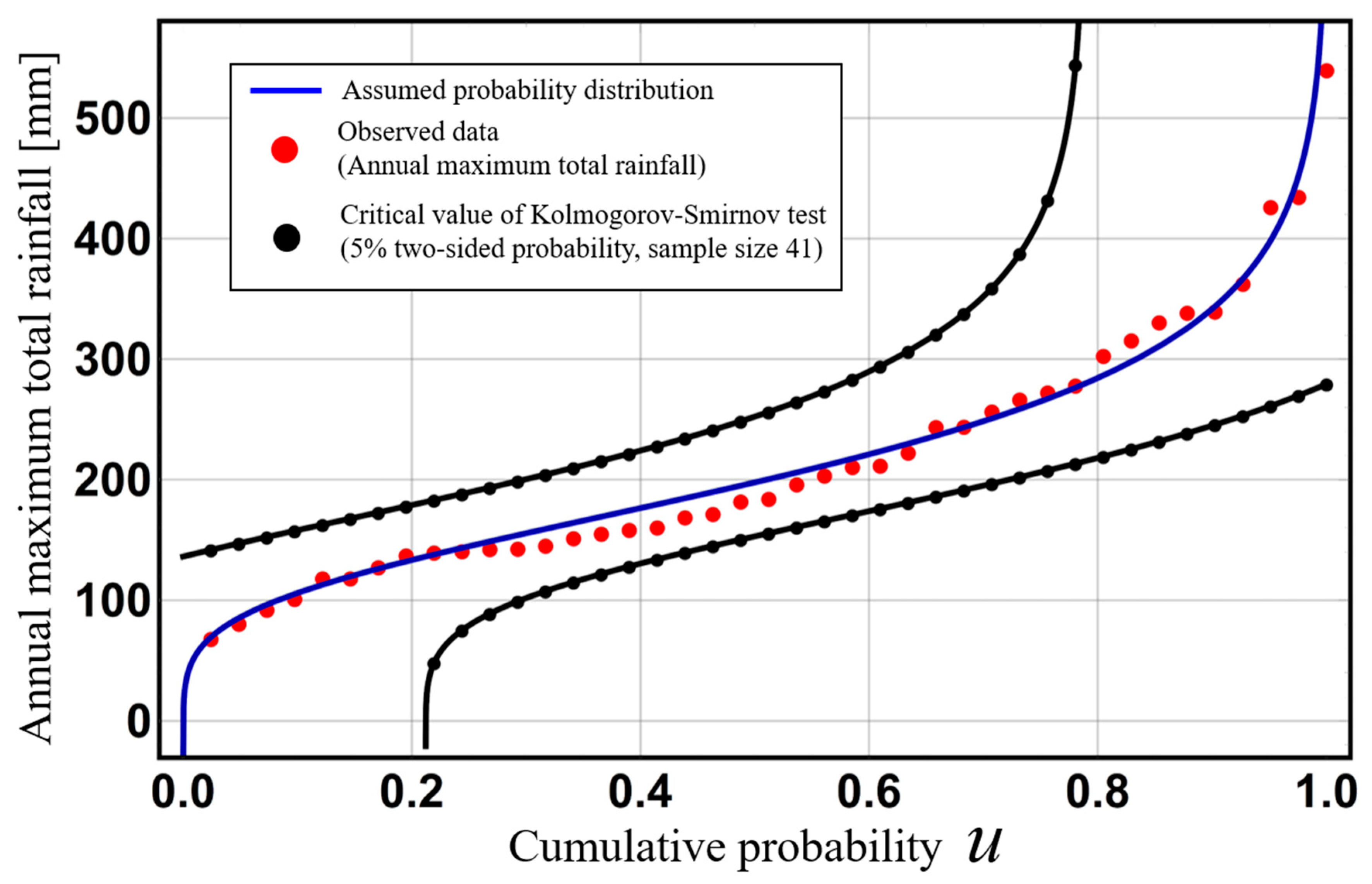
Next, we detail the power of test characteristics of the Kolmogorov–Smirnov test. Figure 3 shows observed data for annual maximum total rainfall for 41 years from 1977 to 2018 in the Kusaki dam basin, a Gumbel distribution that these observed data are assumed to follow, and critical lines in the case of a 5% two-sided probability Kolmogorov–Smirnov test. Here these annual maximum total rainfalls are defined as total rainfall during a 72-h period. In this figure, the acceptance region is narrow in the central part of an assumed distribution. This result illustrates the strong power of the Kolmogorov–Smirnov test at the central part of an assumed probability distribution and its weak power at the tail of the distribution.

3.2. Probability Limit Method Test

This section provides a detailed outline of the probability limit method test. Here, cumulative probability U (= F_X(x)) follows a uniform distribution on interval [0,1]; this uniform distribution is also described as a standard uniform distribution or U [0,1]. We also consider order statistics {u₍₁₎, u₍₂₎, …, u_(n)} constructed of realized values of random variable from U [0,1]. The probability distribution of ith-order statistics from standard uniform distribution becomes a beta distribution with parameter (i, n − i + 1). In Equation (15), F_U(i) (u) expresses the cumulative density function of ith-order statistics U_(i), I_u (i, n − i + 1) representing the cumulative density function of the beta distribution with parameter (i, n − i + 1):

$$\begin{array}{lll}{F}_{U\left(i\right)}\left(i\right)& =& P\left(U_{\left(i\right)}\le u\right)\\ & =& I_u\left(i,n-i+1\right)\end{array}$$

(15)

Here, probability α is defined as the probability used for derivation of probability limit values [20]. The occurrence probability of an extreme U_(i) value is the probability that U_(i) falls in the tail of the beta distribution with parameter (i, n − i + 1). Solution u of equation F_U(i)(u) = α is defined as the lower probability limit value z_L(i) under a standard uniform distribution, while solution u of equation F_U(i)(u) = 1 − α is defined as the upper probability limit value z_U(i) under a standard uniform distribution. Therefore, z_L(i) is the 100α%ile value of the beta distribution with parameter (i, n − i + 1), and z_U(i) is the 100(1 − α)%ile value of the beta distribution with parameter (i, n − i + 1). Probability α_min is defined as

$${\alpha }_{min}=\underset{1\le i\le n}{min}\left\{Min{\left[\begin{array}{c}{I}_u\left(i,n-i+1\right)\\ I_{1-u}\left(n-i+1,\hspace{0.17em}i\right)\end{array}\right]}_{u=u_{(i)}}\right\},$$

(16)

where I_u(i, n − i + 1)|_{u = u(i)} is the nonexceedance probability of ith-order statistics u_(i), and I_{1 − u} (n − i + 1, i)|_{u= u(i)} is the exceedance probability of ith-order statistics u_(i), following the beta distribution with parameter of (i, n − i + 1). Equation (16) expresses a mathematical process to derive probability α_min. The nonexceedance probability and exceedance probability of the order statistics {u₍₁₎, u₍₂₎, _…, u_(n)} are compared, and the smaller of the two probabilities is extracted. As a result, a set of n probabilities is obtained. Probability α_min is the minimum value of these n probabilities. Here, a set of n probabilities is described as {α’₁, α’₂,_…, α’_n}, so probability α_min can be described as α_min = Min{α’₁, α’₂,_…, α’_n}.

Next, the construction method and distributional characteristics of probability α_min are illustrated in detail. Firstly, a set of n random values under the standard uniform distribution are generated, and ensemble sample U_ens. ^j = {u ^j₁, u ^j₂, …, u ^j_n} is constructed from these random values. This procedure is repeated N times, obtaining N sets of samples {U_ens. ¹, U_ens. ², …, U_ens. ^N}. Here, j expresses the sample number (j = 1, 2,…, N). For a sample of U_ens. ^j, the ith-order statistics U^j_(i) under the standard uniform distribution follow a beta distribution with parameter (i, n − i + 1). In the below, the u ^j_(i) that occurs farthest down either tail of the beta distribution with parameter (i, n − i + 1) in a sample of U_ens. ^j is described as u ^j_(i)’ to help clarify the explanation. When u ^j_(i)’ falls in the left tail of the beta distribution with parameter (i, n − i + 1), the nonexceedance probability of u ^j_(i)’ is extracted, so this nonexceedance probability is defined as α_min (j). On the other hand, when u ^j_(i)’ falls in the right tail of beta distribution with parameter (i, n − i + 1), the exceedance probability of u ^j_(i)’ is extracted, and this exceedance probability is defined as α_min (j). The mathematical procedure shown in Equation (16) is applied to the set of N ensemble samples {U_ens. ¹, U_ens. ², …, U_ens. ^N}, obtaining a sample of α_min values {α_min(1), α_min(2), …, α_min(N)}. Here, the order of α_min is so small that α_min is converted to a form of −log₁₀(2α_min) for convenience. For example, the average order of α_min is about 10⁻². 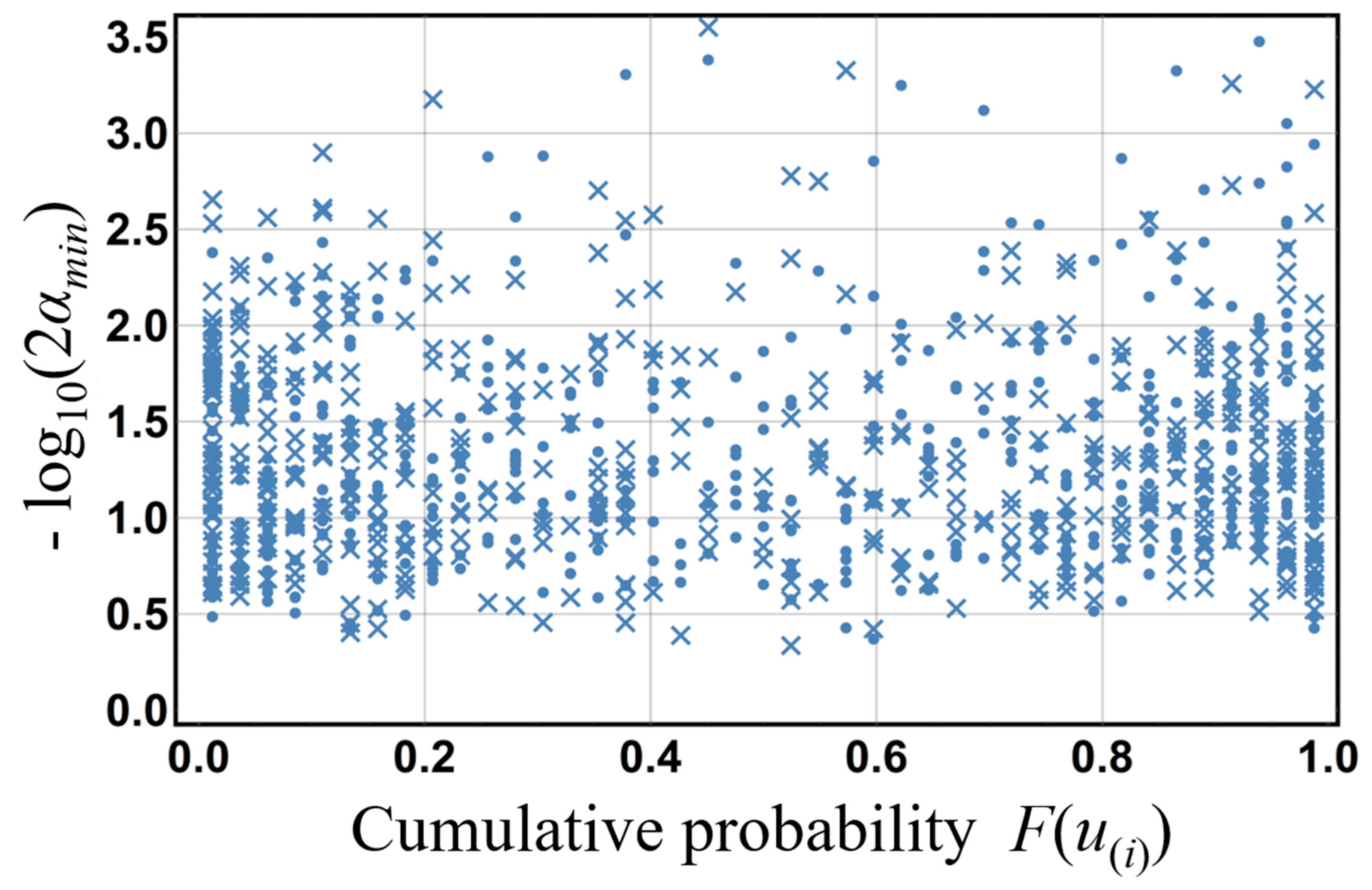Figure 4 shows a 1000-member set of −log₁₀(2α_min) values and the cumulative probability of u_(i) that gives α_min (F(u_(i)) ( = i/n)). In this figure, α_min, which is given by I_u(i, n−i + 1) and the nonexceedance probability, is shown as [×]; α_min, which is given by I_1−u(n−i + 1, i) and the exceedance probability, is shown as [O]. This figure makes clear that α_min is distributed uniformly, and that α_min takes on the value of the nonexceedance and exceedance probabilities with almost equal frequency. To describe probability α corresponding to arbitrary significance levels, empirical representing function χ_emp(u), i.e., the probability representing function of the empirical distribution, is constructed using N − log₁₀(2α_min). An example of this empirical representing function χ_emp(u) for N = 1000 is shown in Figure 5. In the empirical representing function shown in Figure 5, the probability α near the cumulative probability of 1.0 represents the nonexceedance probability or exceedance probability, whichever ith-order statistic occurs more farther down either tail of the beta distribution with parameter (i, n − i + 1). Here, probability α corresponds to a two-sided probability of p representing the elimination of 100(p/2)% from the smaller probability α_min of the nonexceedance probability or exceedance probability, since α_min takes on the value of the nonexceedance and exceedance probabilities with almost equal frequency.

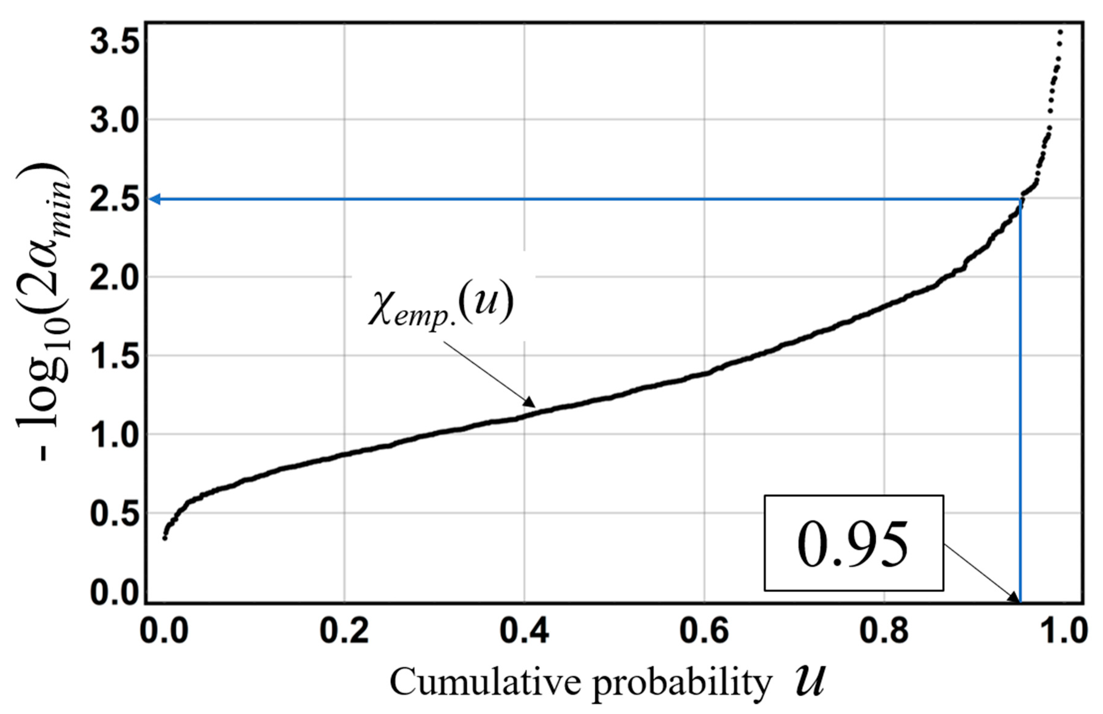
Next, we illustrate the derivation method of probability α corresponding to a 5% two-sided probability in the probability limit method test. Probability α corresponding to a 100(1−α)% two-sided probability is obtained by solving equation χ_emp. (p) = −log₁₀(2α) for α. For example, probability α corresponding to a 5% two-sided probability is derived by solving χ_emp.(0.95) = −log₁₀(2α) = 2.5, resulting in an α value of about 1.5 × 10⁻³ in Figure 5.

The lower probability limit and upper probability limit values under a standard uniform distribution can be derived by using probability α calculated by the method outlined above. Here, in Equation (15), the event (U_(i) ≤ u) means that a value less than u occurs more than i times. Therefore, Equation (17) provides an easier way to calculate the probability limit value in the probability limit method test:

$$F_{U(i)}\left(u\right)={\displaystyle \sum _{j=i}^n\left(\begin{array}{c}n\\ j\end{array}\right)}\hspace{0.17em}\hspace{0.17em}{u}^j{\left(1-u\right)}^{n-j}$$

(17)

The lower probability limit value corresponding to the two-sided probability of p is the one eliminating the occurrence probability of the more extreme (i.e., smaller) ith-order statistics in the beta distribution with parameter (i, n − i + 1). 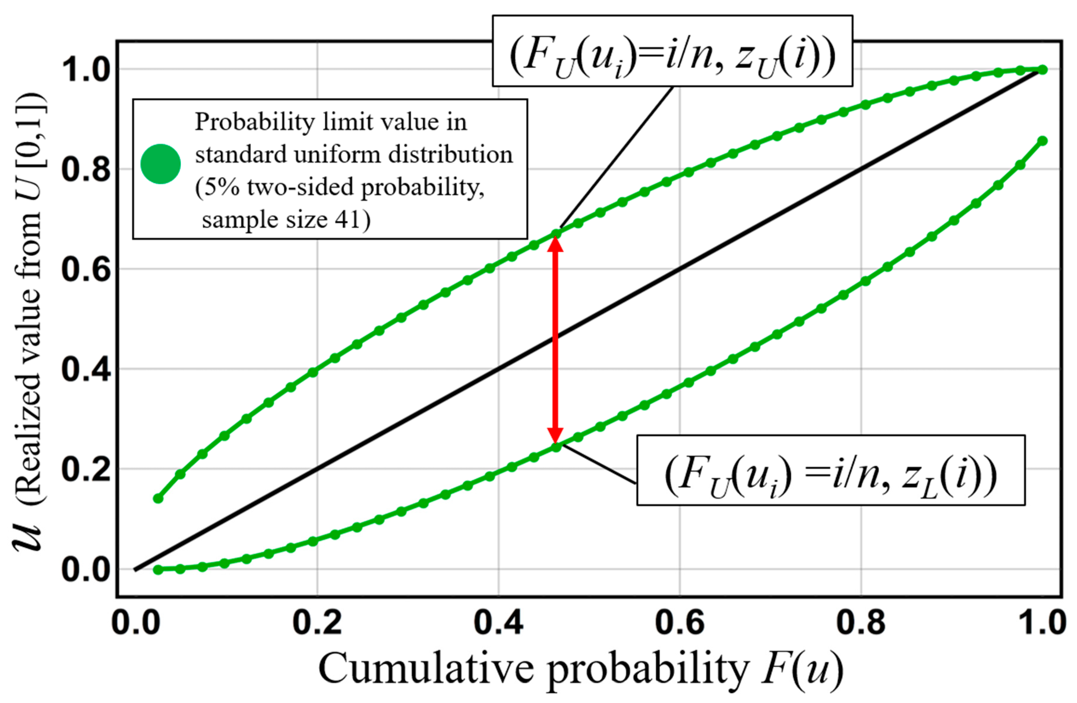Similarly, the upper probability limit value corresponding to the two-sided probability of p is the one eliminating the occurrence probability of the more extreme (i.e., larger) ith-order statistics in the beta distribution with parameter (i, n − i + 1). Values derived by applying the precise cumulative probability F_U(u_(i)) to the probability limit value are defined as the lower probability limit point (F_U(u_(i)), z_L(i)) and the upper probability limit value (F_U(u_(i)), z_U(i)) under the standard uniform distribution. Here, F_U(u_(i)) is defined as i/n. In the standard uniform distribution, the lower probability limit line is defined as an interpolated line of lower probability limit points, while the upper probability limit line is defined as an interpolated line of upper probability limit points for i = 1, 2, …, n. Figure 6 shows probability limit lines for a standard uniform distribution for a 5% two-sided probability and a sample size of 41. This figure shows the range that the ith-order cumulative probability U_(i)(= F_X(X_(i))) can take.

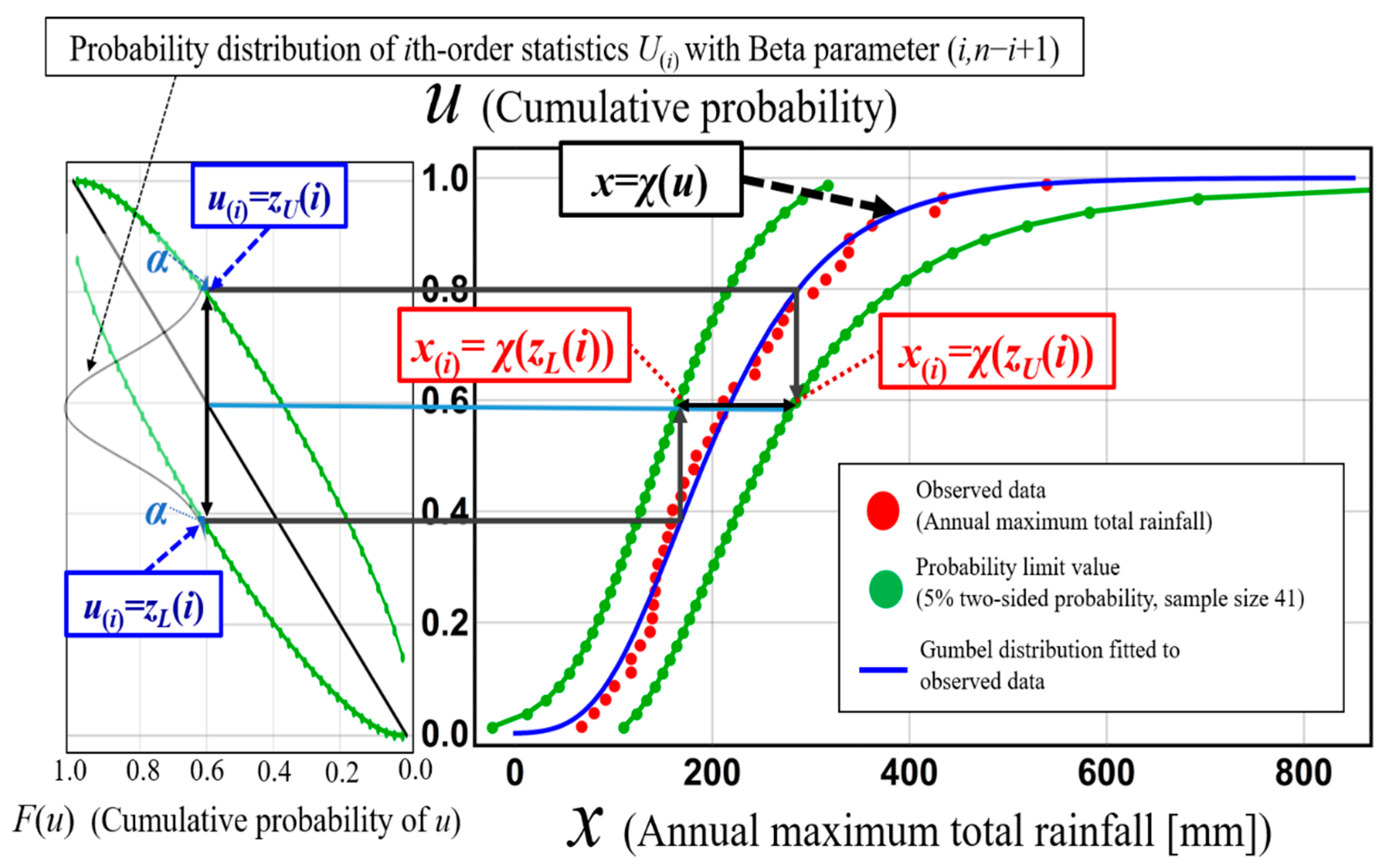
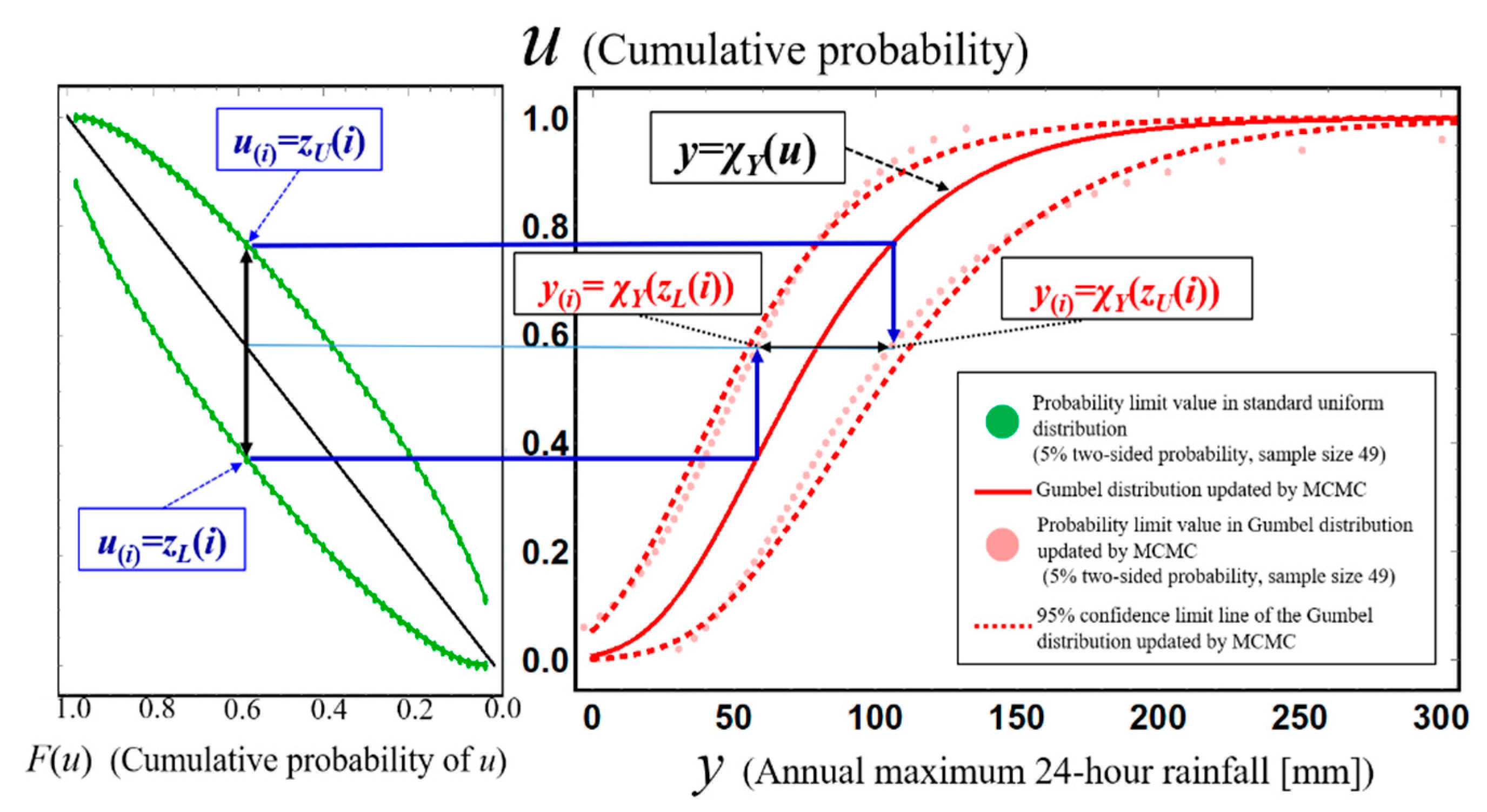
Next, we provide a derivation procedure for the probability limit values of the assumed probability distribution D(X;$\mathit{\theta }$). U follows a standard uniform distribution, and probability limit values are treated as cumulative probability. Therefore, the lower probability limit value in the assumed probability distribution is described by χ_X(z_L(i)), while the upper probability limit in assumed probability distribution is described by χ_X(z_U(i)). Figure 7 shows the construction process of the probability limit line for a 5% two-sided probability for an assumed Gumbel distribution of annual maximum total rainfall for 41 years from 1977 to 2018 in the Kusaki dam basin, Japan. This figure shows that acceptance regions [z_L(i), z_U(i)] for the ith cumulative probability are converted to acceptance regions [χ_X(z_L(i)), χ_X(z_U(i))] for ith-order annual maximum total rainfall X_(i) itself through the representing function of an assumed probability distribution.

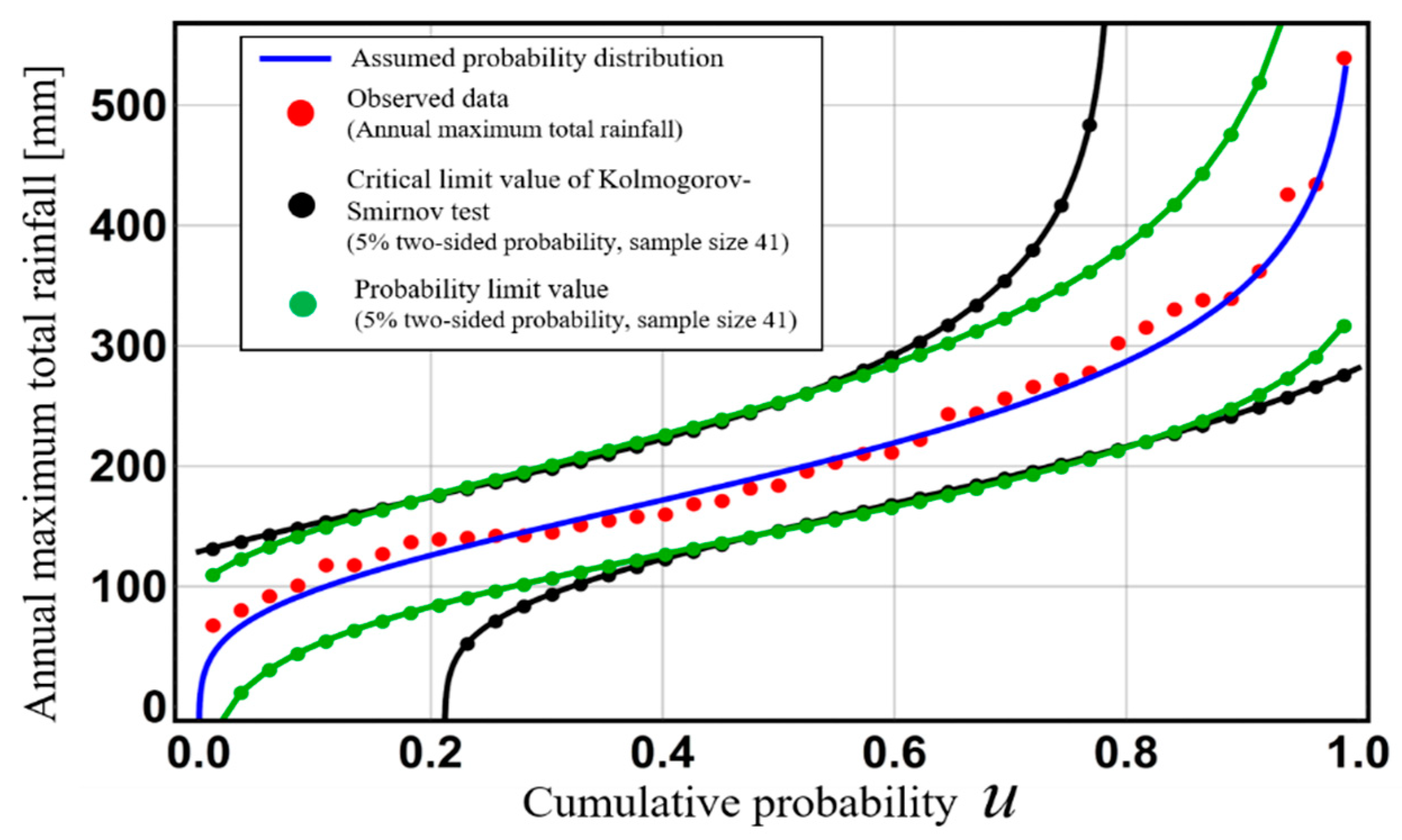
3.3. Power Comparison between Kolmogorov–Smirnov Test and Probability Limit Method Test

Figure 8 shows the critical lines of the Kolmogorov–Smirnov test and probability limit method tests for 5% two-sided probability using the same data. An acceptance region, i.e., the area between the limit lines, expresses how broadly the data are distributed under the adopted hypothesis-testing theory. Based on this figure, the range of the Kolmogorov–Smirnov test’s acceptance region is infinite at the tail of the assumed probability distribution. This means that infinite values of rainfall or river discharge are allowed under Kolmogorov–Smirnov test. The existence of infinite values of rainfall or river discharge does not accord with the real world. On the other hand, the acceptance region in the probability limit method test narrows at the tail of an assumed probability distribution. This means that extreme values corresponding to the tail of an assumed probability distribution can be estimated as an acceptance region with high accuracy. Thus, the power, confidence interval, and prediction interval are interrelated. In general, the greater power the adopted hypothesis-testing theory has, the more precise the confidence and prediction intervals based on the adopted hypothesis-testing theory. The design level for a given hydrological quantity fluctuates dramatically depending on the tail of the adopted distribution. Therefore, since the probability limit method test shows high accuracy at the distribution tails, confidence intervals and prediction intervals in this research are constructed based on probability limit method test to evaluate uncertainties in hydrological statistics.

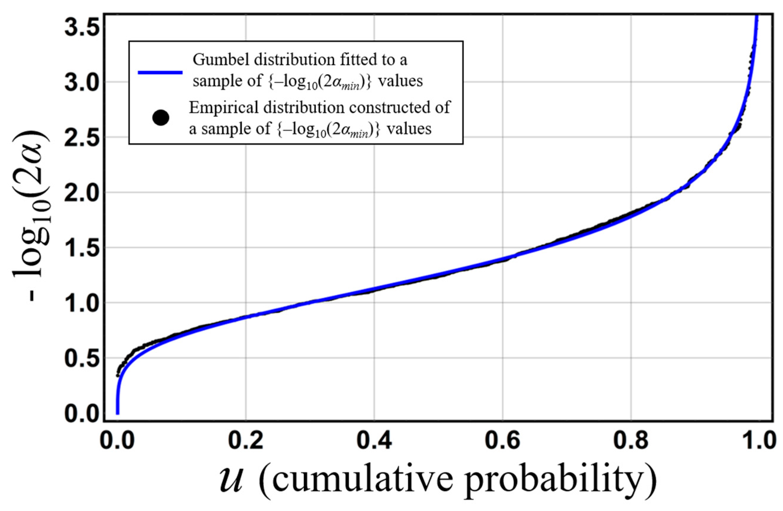
3.4. Construction of Confidence Intervals and Prediction Intervals Based on Probability Limit Method Test

In this section, the construction method for confidence intervals and prediction intervals based on probability limit method tests is illustrated in detail [49]. In this research, probability α is derived from the extreme value distribution fitted to N − log₁₀(2α_min). We note that probability α as used herein differs from that of Moriguti [20]. The reason to adopt an extreme value distribution for a sample of −log₁₀(2α_min) is as follows. Suppose that a sample {α’₁, α’₂,_…, α’_n} is converted to a sample {−log₁₀(2α’₁), −log₁₀(2α’₂), …, − log₁₀(2α’_n)}. In this case, the following relation holds: −log₁₀(2α_min) = Max{−log₁₀(2α’₁) −log₁₀(2α’₂)_…, − log₁₀(2α’_n)}. Then −log₁₀(2α_min) is the maximum value of any sample of the form {−log₁₀(2α’₁) − log₁₀(2α’₂)_…, −log₁₀(2α’_n)}. Maxima of a sample approximately follow an extreme value distribution as sample size increases. Therefore, it is rational to adopt an extreme value distribution for fitting of a sample of −log₁₀(2α_min) values. Figure 9 shows the probability representing function χ_α(u) fitted with a 1000-member set of −log₁₀(2α_min) values. As seen in this figure, χ_α(u) and χ_emp.(u) almost coincide. Therefore, by deriving χ_α(u), confidence intervals can be constructed for arbitrary significance levels. For example, In the case of 5% two-sided probability, probability α for construction of a 95% confidence interval can be obtained by solving χ_α(0.95) = −log₁₀(2α) = 2.5, resulting in an α value of about 1.5 × 10⁻³.

The interval [z_L(i), z_U(i)] is the mathematical range that the cumulative probability of the ith-order statistics derived from random variable series {X₁, X₂, …, X_n} takes. By substituting probability limit values under a standard uniform distribution into the probability representing function χ_X(u), the acceptance region of X _(i) can be constructed in the form [χ_X (z_L(i)), χ_X (z_U(i))]. Therefore, χ_X (z_L(i)) and χ_X (z_U(i)) are the lower and upper probability limit values, respectively, of X_(i), following an adopted probability distribution.

The construction procedure of the 100(1-p)% confidence limit line is as follows. The function form of the adopted probability distribution D(X;$\mathit{\theta }$) is applied to “sample X_L = {χ_X(z_L(1)), χ_X(z_L(2)), …, χ_X(z_L(n))}, constructed of lower probability limit values” and “sample X_U = {χ_X(z_U(1)), χ_X(z_U(2)), …, χ_X(z_U(n))}, constructed of upper probability limit values.” This procedure allows parameter $\mathit{\theta }$ to be estimated. Considering parameter ${\widehat{\mathit{\theta }}}_L$ derived from sample X_L and parameter ${\widehat{\mathit{\theta }}}_U$ derived from sample X_U, the probability distribution D(X;${\widehat{\mathit{\theta }}}_L$) derived from these estimated values is established as the lower confidence limit of D(X;$\mathit{\theta }$), and D(X;${\widehat{\mathit{\theta }}}_U$) is established as the upper confidence limit of D(X;$\mathit{\theta }$). Therefore, in this research, D(X;${\widehat{\mathit{\theta }}}_L$) is defined as the 100(1 − p)% lower confidence limit line, and D(X;${\widehat{\mathit{\theta }}}_U$) is defined as the 100(1 − p)% upper confidence limit line. In addition, the interval between these limit lines is defined as the 100(1 − p)% confidence interval of D(X;$\mathit{\theta }$). In traditional hydrological frequency analysis, the confidence interval is derived from profile likelihood, parametric method, etc. The profile likelihood method assumes that statistics constructed of profile log-likelihood follow a chi-square distribution [50]. Our proposed confidence intervals based on probability limit tests have the advantage of not requiring any assumption, relying instead on analytical construction as much as possible. In addition, hydrological frequency analysis using confidence intervals can be applied to runoff analysis regarding infiltration on a slope [51,52,53].

We next show the construction method for prediction intervals for probability distributions [54]. The acceptance region of the probability limit method test estimates with high accuracy the range of extreme rainfall that could possibly be experienced. Probability limit values can be interpreted as limit values of extreme rainfall at a given significance level. Therefore, when a probability distribution fitted with the greatest number of probability limit values is selected, this probability distribution gives the limiting range of observed data. In addition, it is possible to use this probability distribution to obtain the limit of data as a form of the extrapolated value. This use expresses the prediction of the limit of observed data in future observations, beyond the limits of past concrete observations. Therefore, the probability distribution with the highest goodness-of-fit to probability limit values is defined as the prediction limit line. When the value of the confidence coefficient is near 1.0, the exceedance probability of the upper probability limit value is approximated as p/2 [53]. Because prediction limit values are extrapolated values of probability limit values, it can be assumed that the exceedance probability of the upper prediction limit is almost p/2. Therefore, introducing the risk calculated by the above framework, it is possible to compare the occurrence risk of heavy rainfall to risk in some other fields. In addition, the occurrence risk of a heavy rainfall event can be quantified using the prediction interval. The risk is expressed as a product of the targeted return period and the one-sided probability of the prediction interval [54]. Here, Knight [55] defined risk as the phenomenon whose uncertainty is quantified as a form of the probability distribution. Considering this definition, risk is expressed as the occurrence risk of heavy rainfall that falls near any part of the upper prediction limit line with a high confidence coefficient and is evaluated as a phenomenon corresponding to the tail distribution of probable rainfall itself, which can be estimated using the prediction interval.

4. Update of Extreme Value Distribution Using Markov Chain Monte Carlo Method

This section presents a method for updating the extreme value distribution derived from the past observed data. The update provides an extreme value distribution for future climate and constructs its confidence interval and prediction interval by using a Markov Chain Monte Carlo method [56]. Here, Bayes’ theorem is used to express the posterior distribution f(θ|x) of parameter θ is expressed as

$$f\left(\mathit{\theta }|x\right)=\frac{f\left(x|\mathit{\theta }\right)f\left(\mathit{\theta }\right)}{{\displaystyle {\int }_{\Theta }f\left(x|\mathit{\theta }\right)f\left(\mathit{\theta }\right)d\mathit{\theta }}}\hspace{0.17em}\propto f\left(x|\mathit{\theta }\right)f\left(\mathit{\theta }\right)$$

(18)

where f(θ) is the prior distribution of θ, and f(x|θ) is the likelihood function. Equation (18) shows that a prior distribution, which expresses prior information, is updated to a posterior distribution as information for parameter θ accumulates as each additional datum is observed. In general, the posterior distribution of an extreme value distribution of parameter θ cannot be derived from its prior distribution analytically using Bayes’ theorem. Therefore, in this research, a Markov Chain Monte Carlo method is adopted to numerically derive posterior distributions of parameters. In addition, the posterior distribution of the parameter of the Gumbel distribution fitted to observed data is derived using the Metropolis method, one of the Markov Chain Monte Carlo methods [57]. Observed annual maximum 24-h rainfall data for the Tokoro river basin, Japan, over 49 years from 1962 to 2010 are used as the analytical data.

4.1. Outline of Metropolis Method

The Metropolis method procedure is as follows [57]:

(1)

Set initial value of parameter θ.

(2)

Select random value θ’ from proposed distribution q(θ), which provides candidate values for the parameter.

(3)

Calculate probability γ as expressed by

$$\gamma =Min\left\{\frac{f\left(\mathit{\theta }\hspace{0.17em}’|x\right)}{f\left(\mathit{\theta }|x\right)},\hspace{0.17em}\hspace{0.17em}1\right\}.$$

(19)

(4)

Transition θ to θ’ with probability γ, updating θ to θ’. This update is conducted with probability (1−γ).

(5)

Repeat steps (2) through (4), inclusive.

(6)

When convergence of sample series of θ is recognized, iterative calculation is stopped.

Here, θ is the parameter of interest, f(θ) is the prior distribution of θ, f(x|θ) is the likelihood function, and f(θ|x) is the posterior distribution.

4.2. Outline of Ensemble Climate Projection Data

In this research, dynamical downscaled data of the regional experiment from the database for Policy Decision making for Future climate change (d4PDF [58,59]) constructed by Yamada et al. are used [23,25,26]. This regional experiment of d4PDF was constructed of ensemble data calculated from a regional climate model with a horizontal resolution of 20 km. More precisely, this regional experiment was constructed from past experiments targeting the 60 years from 1951 to 2010 and the +4K experiment, which assumes a condition of increasing of global average temperature by 4K from the era of industrial revolution and targets the 60 years from 2051 to 2110. The past experiment included 50 ensemble members perturbing sea ice conditions, sea surface temperatures, and initial conditions, for a total of 60 years × 50 members = 3000 years. The +4K experiment included 6 sea surface temperature patterns and 15 ensemble members perturbing of these patterns of sea surface temperature, for a total of 60 years × 6 sea surface patterns × 15 members = 5400 years. The horizontal, high-resolution database this research used was composed of ensemble data derived by dynamical downscaling the regional experiment’s data of d4 PDF to a horizontal resolution, 5 km. In this research, the geographic subset corresponding to the position of the Tokoro river basin was extracted from the +4K experiment’s annual maximum 24-h rainfall data and used for Bayesian update of the Gumbel distribution fitted to past observed data. The 6 patterns of sea surface temperature were calculated by 6 main models used for Coupled Model Inter Comparison Project Phase 5 (CMIP5). In this research, observed data were treated as a sample of a population of past climate. Here

Table 2. Meaning of acronym.

Acronym	Meaning
d4PDF	a database for Policy Decision making for Future climate change
CMIP5	Coupled Model Inter-comparison Project Phase 5

shows meanings of acronyms in Section 4.

4.3. Results from Metropolis Method

Initial values of parameters in the Metropolis method, estimated by maximum likelihood, were derived by fitting a Gumbel distribution to observed data. The prior distributions for each parameter are assigned as noninformative uniform distribution. This research assumes that initial value of MCMC is decided reliably from past observed data as most likelihood estimated value, although detailed information of prior distribution is unknown. Figure 10 shows the results of the Metropolis method. Here, 5400 years of annual maximum 24-h rainfall data from the +4K experiment were substituted into the likelihood function. Figure 10 shows a sample series of posterior distributions of parameters becoming almost stable, with very few rejection values to be deleted from the calculation (burn-in). Therefore, verification of the application of the Metropolis method is shown. In the future research, identification of prior distribution will be analyzed in the perspective of past observed information. More concretely, ensemble climate simulations are conducted for past climate, and prior distribution could be estimated by using parameters from a lot of simulated rainfalls in the past experiment.

4.4. Construction of Predicted Distribution for Future Climate

The predicted distribution for extreme values can be expressed as

$$P\left(Y\le y|\mathit{x}\right)={\displaystyle {\int }_{\Theta }F\left(Y\le y|\mathit{\theta }\right)f\left(\mathit{\theta }|\mathit{x}\right)d\hspace{0.17em}\mathit{\theta }},$$

(20)

where Y is a random variable which representing extremes in future climate, P(Y ≤ y|x) represents the cumulative density function of the predicted distribution for extreme values, F(Y ≤ y|θ) represents the cumulative density function of random variable Y given θ, f(θ|x) represents the posterior density of the parameter derived from observed data, and χ_Y(u) represents the probability representing function of the predicted distribution for extreme values. When sample series of the parameter are derived using the MCMC method, a predicted distribution for extreme values is expressed by Equation (21).

$$P\left(Y\le y|\mathit{x}\right)\approx \frac{1}{s}{\displaystyle \sum _{i=1}^s{F}_Y\left(y|{\mathit{\theta }}_i\right)}$$

(21)

Here F_Y(y) is an assumed probability distribution of a population of unknown future data. Equation (21) shows that the cumulative density function P(Y ≤ y|x) of the predicted distribution for extreme values can be derived from approximately the average of cumulative probability of future observed data y. More precisely, the average can be obtained by dividing the summation of each cumulative probability of future observed data F_Y(y|θ_i) with total number of adopted parameters. Here, θ_i is a generated parameter by MCMC, s is the number derived by subtracting the number of rejected samples from the total number of MCMC trials.

In this research, a Gumbel distribution was adopted as the population distribution of unknown future data. The MCMC iteration number was 41,000, and the total number of burn-in intervals was 1000. Therefore, s was 40,000, which is the number derived by subtracting 1000 from 41,000. The confidence interval of the Bayesian probability distribution updated by MCMC (i.e., the predicted distribution of probability distribution fitted to past observed data) can be also constructed by the method based on the probability limit method test shown in Section 4. Figure 11 shows the construction process of the 95% confidence interval of the Gumbel distribution, which is Bayesian-updated by MCMC, incorporating the +4K annual maximum 24-h rainfall data. In this figure, probability limit values under the standard uniform distribution are green points, while those of the +4K experiment are light red points. The Gumbel distribution, which is Bayesian-updated by applying the MCMC method to the +4K experiment, is a solid red line, and the 95% confidence limit line of this Gumbel distribution is a dotted red line. The probability limit values under the standard uniform distribution were determined based on the total number of observed data points. Therefore, probability limit values under the standard uniform distribution were subject to the same conditions under past climate and future climate.

5. Results and Discussion

5.1. Update of Confidence Interval Based on Bayesian Method Using Ensemble Climate Projection Data

Figure 12 shows the analytical data (black points), Gumbel distribution fitted to the observed data (blue solid line), 95% confidence interval of this Gumbel distribution for past climate (blue range), Bayesian-updated Gumbel distribution, and 95% confidence interval of this Bayesian-updated Gumbel distribution. From the overlapping range of the past and future climate intervals’ distributions, it is probable that rainfall maxima observed in past climate could occur in future climate. Notably, the confidence interval of future climate is wider than that of past climate, and probable rainfall will increase in future climate. Moreover, considering the return period of 100 years, which is often used as the design level in Japan, the 100-year annual maximum 24-h rainfall in future climate (224.6 mm) is about 42% greater than in past climate (157.7 mm). In addition, the 95% upper confidence limit value in future climate (294.4 mm) is an about 48% greater than in past climate (198.8 mm). By quantifying the future change ratio for the design level rainfall, it becomes clear that by updating the confidence interval, we can improve the feasibility of future rainfall predictions under climate change accompanied by global warming.

Moreover, the uncertainty of T-year rainfall is quantified in river planning of a return period of T years, and record rainfall, which cannot be meaningfully evaluated using traditional methods, is interpreted as a phenomenon within the confidence interval. In other words, the confidence interval can rationally evaluate the return period of heavy rainfall. Furthermore, the exceedance probability of the upper confidence limit value is expressed as the product of the targeted return period and the exceedance probability of confidence limit value [49]. In river plannings, whose design level is T-year, the risk of rainfall exceeding a 100(1 − p)% upper confidence limit value is quantified as [(1/T) × (p/2)] [49]. For example, the probability of exceedance of the 95% upper confidence limit value of a 100-year annual maximum total rainfall is 1/100 × 2.5% = 0.025%. Like this framework of confidence interval, the risk of occurrence of heavy rainfall which cannot be evaluated in the traditional way is quantified. In addition, the risk derived from the above mentioned framework can be compared with risk in another fields because the order of risk derived from above mentioned risk is almost the same order of risk in other fields such as death by traffic accident, airplane accident, etc. This result proposes a feasibility of relative evaluation in river planning corresponding to climate change.

5.2. Goodness-of-Fit Evaluation of Both Confidence Intervals Based on Probability Limit Method Test and Physical Monte Carlo Method

To clarify the uncertainty of probable rainfall, histograms of probable rainfall value in both past climate and future climates were used. To compare the goodness-of-fit of confidence intervals for both past and future climate, statistical resampling was conducted to both the past experiment data and the future data. More precisely, 5000 resampled samples were generated by the following process. For the past data, annual maximum 24-h rainfall data for 3000 years were resampled into 49-year timelines, equal in length to the total number of observed years. Five thousand such resampled samples were generated. The same process was conducted on the future data. Next, by fitting a Gumbel distribution to these resampled samples for both past and future climate, a probability evaluation was conducted. Figure 13 shows the Gumbel distribution fitted to observed data (solid blue line), the 95% confidence interval of this Gumbel distribution in past climate (interval between dotted blue lines), and Gumbel distributions fitted to each of the 5000 resampled samples for past climate (thin green lines). Figure 14 also shows the Bayesian-updated Gumbel distribution for future climate (solid red line), the 95% confidence interval of this Bayesian-updated Gumbel distribution (interval between dotted red lines), and Gumbel distributions fitted to each of the 5000 resampled samples for future climate (thin orange lines).

Based on Figure 13 and Figure 14, the uncertainty of probable rainfall is clarified as a range, and this range fits a theoretical confidence interval derived by applying the probability limit method test. In particular, the confidence interval for past climate was derived by a completely theoretical method of the probability limit method test and does not use the information from the horizontal, high-resolution database [23,25,26]. Therefore, the good fit between the confidence interval based on the probability limit method test and that based on the physical Monte Carlo method suggests the usefulness of this test. Here, the confidence interval based on the physical Monte Carlo method is constructed from the lower confidence limit 100(p/2) %ile value and the upper confidence limit 100(1 − p/2) %ile value. These confidence limit values are derived from an empirical distribution of quantiles of probability distributions fitted to the abovementioned resampled samples. Next, goodness-of-fit for each confidence interval was evaluated in terms of coverage probability. Coverage probability is defined as the proportion of targeted estimated statistics falling within the confidence interval. Therefore, coverage probability as used here was the proportion of the distribution of probable rainfall that fell within the confidence interval based on the probability limit method test. The accuracy of the confidence interval could be quantified by calculating the coverage probability. More precisely, a confidence interval with a rational coverage probability whose value is close to an adopted confidence coefficient is desirable [60]. For example, when a 95% confidence interval is constructed, and its coverage probability is about 95%, then the accuracy of this confidence interval is quite good. Figure 15 shows the empirical probability distribution of 100-year probable annual maximum 24-h rainfall derived from resampled samples of past data vs. the 95% confidence interval based on the probability limit method test for past climate using actual observed data. The coverage probability of the 95% confidence interval (the range between the two blue dotted lines) in Figure 15 is 95.5%. Figure 16 shows the empirical probability distribution of 100-year probable annual maximum 24-h rainfall derived from resampled samples of future projected data vs. the 95% confidence interval based on the probability limit method test for future climate. For future climate, the coverage probability is 94.3%. Moreover, in the cases of other return periods, confidence intervals based on the probability limit method test included distributions of probable rainfall derived with high accuracy from the physically based Monte Carlo method using the horizontal high-resolution database [23,25,26].

5.3. Update of Prediction Interval Based on a Bayesian Method Using Ensemble Climate Projection Data

To construct the prediction interval, it is necessary to adopt probability distribution with the best goodness-of-fit for the sample of probability limit values. For that reason, the relation between probability limit values, past experiment data, and future experiment data were analyzed. The validity of the prediction interval proposed herein can be demonstrated by showing that the acceptance region estimating the degree of instability of ith-order statistics of extreme rainfall as a range based on the probability limit method test fit the distribution of calculated order statistics derived from the ensemble database.

The comparison between probability limit values derived from observed data and the regional experiment’s past experiment data was conducted via a probability plot. Figure 17 shows a Gumbel distribution fitted to observed data (blue line), probability limit values with 5% two-sided probability for past climate (blue points), and empirical distributions of resampled samples of the regional experiment’s past data (green points; 500 examples are shown). Figure 18 shows a Bayesian-updated Gumbel distribution for future climate (solid red line), probability limit values for 5% two-sided probability for past climate (blue points), probability limit values for 5% two-sided probability for future climate (red points), and empirical distributions of resampled samples of regional experiment’s future data (brown points; 500 examples are shown). Figure 17 shows that most of the instability derived from the regional experiment’s past data is included in the acceptance region constructed from both lower and upper probability limit values. In addition, based on Figure 18, the degree of instability derived from the regional experiment’s future data almost coincides with the acceptance region of the probability limit method test with 5% two-sided probability. For that reason, the range of distribution of order statistics derived from the physical Monte Carlo method and from the acceptance region of the probability limit method test are almost identical. These results mean that the magnitude of outliers which we could have experienced in the past or will experience in the future are estimated by the theory of probability limit method.

To clarify the goodness-of-fit between the two ranges, the coverage probability of distribution of order statistics within an acceptance region for 5% two-sided probability was calculated. When coverage probability of an acceptance region for 5% two-sided probability was near 95%, the goodness-of-fit between the two ranges was high. Figure 19 shows an acceptance region for 5% two-sided probability derived from a Gumbel distribution fitted to observed data vs. a frequency distribution of 49th-order statistics derived from 5000 resampled samples of the regional past experiment’s data. In this case, the coverage probability was 99.9%, showing the usefulness of the probability limit method test. Furthermore, Figure 20 shows an acceptance region for 5% two-sided probability derived from a Bayesian-updated Gumbel distribution vs. the frequency distribution of 49th-order statistics derived from 5000 resampled samples of the regional experiment’s future data. The coverage probability of the acceptance region for 5% two-sided probability derived from the Bayesian-updated Gumbel distribution was 98.7%, again showing the usefulness of the probability limit method test even for future climate. These findings demonstrate that an acceptance region of probability limit method can estimate the degree of instability with high accuracy. For that reason, it is possible to construct the degree of instability of probable rainfall beyond the observation period; this is defined as the prediction limit line in this research by extrapolation of the probability distribution that shows the best goodness-of-fit for probability limit values.

Here, Figure 21 provides the construction process for the 95% prediction interval for future climate. This figure shows, the probability limit values (green points), the Gumbel distribution that has been Bayesian-updated by applying the MCMC method to the +4K experiment (solid red line), and the 95% limit line for future observed data (a dot-dashed red line). From this figure, it is clear that the prediction limit lines constructed by fitting probability distributions coincide well with probability limit values.

Next, we estimate prediction interval in future climate and analyze characteristics of it. Figure 22 shows observed data (black points), a Gumbel distribution fitted to observed data (blue line), a 95% prediction interval based on the probability limit method test for past climate (blue range), a Bayesian-updated Gumbel distribution derived by applying the MCMC method to a Gumbel distribution fitted to observed data (solid red line), and a 95% prediction interval based on the probability limit method test for future climate (red range). From the overlapping range of the two prediction intervals, it can be recognized that annual maximum 24-h rainfall values from past climate could well occur in future climate with some probability. In addition, the prediction interval for future climate takes on a wider range than that of past climate, showing the occurrence risk of heavy rainfall increases in future climate. Moreover, considering the return period of 100 years, the 95% upper prediction limit value for future climate (437.9 mm) is about 56% greater than for past climate (280.7 mm). By updating the prediction interval, we can evaluate the future scale and occurrence risk of heavy rainfall while accounting for continuing global warming.

6. Summary

Confidence intervals quantify the degree of instability of the adopted probability distribution, and risks in river planning can be expressed by considering confidence interval ranges. Prediction intervals quantify the range that future observed data could take, making it possible to estimate the future occurrence risk and scale of heavy rainfall. This paper provided a construction method for confidence intervals and prediction intervals based on the probability limit method test, illustrating its actual application. This research also showed harmonic relation between confidence intervals based on a physical Monte Carlo method using high-resolution database and confidence intervals based on mathematical theory, namely the probability limit method test. This result suggests the validity of results of ensemble climate simulations from the perspective of theory. It also implies the feasibility of introducing ensemble climate projection data into flood control management.

The main results of this research are as follows.

(1)

A construction method of confidence intervals and prediction intervals based on the probability limit method test is shown. This method has the advantage of constructing both intervals analytically as much as possible, rather than from parametric assumptions.

(2)

In traditional hydrological frequency analysis, probable rainfall is calculated deterministically. On the other hand, by introducing confidence intervals and prediction intervals proposed herein, it becomes possible to estimate the range of probable rainfall and the occurrence probability of heavy rainfall that would otherwise be treated as unexpected in traditional analysis.

(3)

Confidence intervals and prediction intervals make it possible to evaluate the risk of heavy rainfall and compare it meaningfully to risks in other fields.

References

1. Stedinger, J.R.; Vogel, R.M.; Foufoula-Georgiou, E. Frequency analysis of extreme events. In Handbook of Hydrology; Maidment, D., Ed.; McGraw-Hill Professional: New York, NY, USA, 1993; Chapter 18; pp. 18.1–18.66. [Google Scholar]
2. Fisher, R.A.; Tippett, L.H.C. Limiting forms of the frequency distribution of the largest or smallest member of a sample. Proc. Camb. Philos. Soc. 1928, 24, 180–190. [Google Scholar] [CrossRef]
3. Gumbel, E.J. The return period of flood flows. Ann. Math. Stat. 1941, 12, 163–190. [Google Scholar] [CrossRef]
4. Gnedenko, B.V. Sur La Distribution Limite Du Terme Maximum D’Une Serie Aleatoire. Ann. Math. Second Ser. 1943, 44, 423–453. [Google Scholar] [CrossRef]
5. Von Mises, R. La distribution de la plus grande de n values. Rev. Math. Union Interbalkanieque 1936, 1, 141–160. [Google Scholar]
6. Jenkinson, A.F. The frequency distribution of the annual maximum (or minimum) values of meteorological elements. Quart. J. R. Meteorol. Soc. 1955, 81, 158–171. [Google Scholar] [CrossRef]
7. Gumbel, E.J. Statistics of Extremes; Columbia University Press: New York, NY, USA, 1958. [Google Scholar]
8. Coles, S. An Introduction to Statistical Modeling of Extreme Values; Springer: London, UK, 2001. [Google Scholar]
9. de Haan, L.; Ferreira, A. Extreme Value Theory: An Introduction; Springer: New York, NY, USA, 2006. [Google Scholar]
10. Takara, K.; Takasao, T. Criteria for Evaluating Probability Distribution Models in Hydrologic Frequency Analysis. J. Jpn. Soc. Civ. Eng. 1988, 393, 151–160. [Google Scholar]
11. Takara, K. Recent advancement and perspectives of hydrologic frequency analysis. J. Jpn. Soc. Hydrol. Water Resour. 1998, 11, 740–756. [Google Scholar] [CrossRef]
12. David, M.H. On the probability of extreme rainfall events. Bull. Am. Meteor. Soc. 1973, 54, 1013–1018. [Google Scholar]
13. The Federal Interagency Floodplain Management Task Force. Floodplain Management in the United States: An Assessment Report, Volume 2: Full Report. 1992. Available online: https://www.hsdl.org/?abstract&did=456501 (accessed on 31 August 2020).
14. Interagency Floodplain Management Review Committee (U.S.). Sharing the Challenge, Floodplain Management into the 21st Century, Report of the Interagency Floodplain Management Review Committee to the Administration Floodplain Management Task Force. 1994. Available online: https://fas.org/irp/agency/dhs/fema/sharing.pdf (accessed on 31 August 2020).
15. United States Army Corps of Engineer; United States Office of the Assistant Secretary of the Army (Civil Works). Annual Report of Fiscal Year 2011 of the Secretary of the Army on Civil Works Activities (1 October 2010–30 September 2011). 2011. Available online: https://cdm16021.contentdm.oclc.org/digital/collection/p16021coll6/id/2125 (accessed on 31 August 2020).
16. Environment Agency (United Kingdom). Planning for Flood Risk Management in the Thames Estuary, Technical Scoping Report. 2003. Available online: http://www.espace-project.org/part1/publications/reading/espace/docs/Techncial%20Scoping%20Report-March2003.pdf (accessed on 31 August 2020).
17. Ministry of Transport and Water Management (Netherlands). National Water Plan 2009–2015. 2009. Available online: http://publicaties.minienm.nl/documenten/national-water-plan-2009-2015#:~:text=This%20National%20Water%20Plan%20outlines,various%20types%20of%20water%20use (accessed on 31 August 2020).
18. Ministry of Transport, Public Works and Water Management, Directorate-General of Public Works and Water Management (Netherlands). Annual Report Rijkswaterstaat 2013, 2014. Available online: http://publicaties.minienm.nl/documenten/annual-report-rijkswaterstaat (accessed on 31 August 2020).
19. Kind, J.M. Economically efficient flood protection standards for the Netherlands. J. Flood Risk Manag. 2012, 7, 103–117. [Google Scholar] [CrossRef]
20. Moriguti, S. Testing Hypothesis on Probability Representing Function—Kolmogorov–Smirnov Test Reconsidered. Jpn. J. Stat. Data Sci. 1995, 25, 233–244. [Google Scholar]
21. Itokawa, K.; Arakawa, T.; Okabe, M.; Yamada, T. A study on periodicity and frequency of occurrence of extreme value rainfall. J. Inst. Sci. Eng. 2011, 23, 51–57. [Google Scholar]
22. Yamada, T.J.; Seang, C.N.; Hoshino, T. Influence of the long-term temperature trend on the number of new records for annual maximum daily precipitation in Japan. Atmosphere 2020, 11, 371. [Google Scholar] [CrossRef] [Green Version]
23. Yamada, T.J.; Hoshino, T.; Masuya, S.; Uemura, F.; Yoshida, T.; Omura, N.; Yamamoto, T.; Chiba, M.; Tomura, S.; Tokioka, S.; et al. The influence of climate change on flood risk in Hokkaido. Adv. River Eng. 2018, 24, 391–396. [Google Scholar]
24. Hoshino, T.; Yamada, T.J.; Kawase, H. Evaluation for Characteristics of Tropical Cyclone Induced Heavy Rainfall over the Sub-basins in The Central Hokkaido, Northern Japan by 5-km Large Ensemble Experiments. Atmosphere 2020, 11, 435. [Google Scholar] [CrossRef]
25. Ministry of Land, Infrastructure, Transport, and Tourism (MLIT). Flood Control Technology Review Meeting Considering the Climate Change in Hokkaido Region. Available online: https://www.hkd.mlit.go.jp/ky/kn/kawa_kei/splaat000001offi.html (accessed on 31 August 2020).
26. Yamada, T.J. Adaptation Measures for Extreme Floods Using Huge Ensemble of High-Resolution Climate Model Simulation in Japan. Summary Report on the Eleventh Meeting of the Research Dialogue 2019, 28–30, UNFCCC Bonn Climate Change Conference, Bonn, Germany (19 June 2019). Available online: https://unfccc.int/documents/197307 (accessed on 31 August 2020).
27. Efron, B. The Jackknife, the Bootstrap, and Other Resampling Plans; Society for Industrial and Applied Mathematics: Philadelphia, PA, USA, 1982. [Google Scholar]
28. Khaliq, M.N.; Ourada, T.B.M.J.; Ondo, J.C.; Gachon, P.; Bobee, B. Frequency analysis of a sequence of dependent and/or non-stationary hydrometeorological observations: A review. J. Hydrol. 2006, 329, 534–552. [Google Scholar] [CrossRef]
29. Linyin, C.; Amir, A.; Eric, G.; Richard, W.K. Non-stationary extreme value analysis in a changing climate. Clim. Chang. 2014, 127, 353–369. [Google Scholar]
30. Hayashi, H.; Tachikawa, Y.; Shiiba, M. Non-stationary hydrologic frequency analysis using time dependent parameters and its model selection. J. Jpn. Soc. Civ. Eng. (Hydraul. Eng.) 2015, 71, I_28–I_42. [Google Scholar]
31. Wiel, K.; Wanders, N.; Selten, F.M.; Bierkens, M.F.P. Added value of large ensemble simulations for assessing extreme river discharge in a 2 °C warmer world. Geophys. Res. Lett. 2019, 46, 2093–2102. [Google Scholar] [CrossRef] [Green Version]
32. United Nations Framework Convention on Climate Change. Adoption of the Paris Agreement (Report No. FCCC/CP/2015/L.9/Rev.1). 2015. Available online: https://unfccc.int/resource/docs/2015/cop21/eng/l09r01.pdf (accessed on 4 September 2020).
33. KNMI, Deltares. Wat Betekenen de Nieuwe Klimaatscenario’s voor de Rivierafvoeren van Rijn en Maas? 2015, p. 15. Available online: http://publications.deltares.nl/1220042_004.pdf (accessed on 4 September 2020).
34. Takeuchi, K. Contributions on Theory of Mathematical Statistics; Springer: Tokyo, Japan, 2020. [Google Scholar]
35. Kitano, K.; Takahashi, R.; Tanaka, S. Prediction interval for the largest extreme encountered in the future time, distinguished from the confidence interval for a certain level given by return period. J. Jpn. Soc. Civ. Eng. (Hydraul. Eng.) 2013, 69, I_271–I_276. [Google Scholar]
36. Coles, S. Anticipating catastrophes through extreme value modelling. Appl. Statist. 2003, 52, 405–416. [Google Scholar] [CrossRef]
37. Kitano, T.; Takahashi, R.; Tanaka, S. Bayesian Prediction for Extremes of Precipitation in a Mutually Complementary Manner with Information by Maximum Likelihood Estimation. J. Jpn. Soc. Civ. Eng. (Hydraul. Eng.) 2016, 72, I_463–I_468. [Google Scholar]
38. Neyman, J. Outline of a Theory of Statistical Estimation Based on the Classical Theory of Probability. Philos. Trans. R. Soc. A 1937, 236, 333–380. [Google Scholar]
39. Kolmogorov, A. Sulla Determinazione Empiri-ca di una Legge di Distribuzione. Inst. Ital. Attuari Giorn. 1933, 4, 83–91. [Google Scholar]
40. Smirnov, N. Ob uklonenijah empiriceskoi krivoi raspredelenija. Recl. Math. (Mathmaticeskii Sb.) 1939, 6, 3–26. [Google Scholar]
41. Anderson, T.W.; Darling, D.A. Asymptotic theory of certain “goodness-of-fit” criteria based on stochastic processes. Ann. Math. Stat. 1952, 23, 193–212. [Google Scholar] [CrossRef]
42. Stephens, M.A. EDF Statistics for Goodness of Fit and Some Comparisons. J. Am. Stat. Assoc. 1974, 69, 730–737. [Google Scholar] [CrossRef]
43. NIST/SEMATECH. e-Handbook of Statistical Methods. Anderson-Darling Test. Available online: https://www.itl.nist.gov/div898/handbook/eda/section3/eda35e.htm (accessed on 31 August 2020).
44. Moriguti, S. Probability Representing Function; Tokyo University Press: Tokyo, Japan, 1995. [Google Scholar]
45. Feller, W. On the Kolmogorov–Smirnov limit theorems for empirical distributions. Ann. Math. Stat. 1948, 19, 177–189. [Google Scholar] [CrossRef]
46. Massey, F.J., Jr. A note on the estimation of a distribution function by confidence limits. Ann. Math. Stat. 1950, 21, 116–119. [Google Scholar] [CrossRef]
47. Birnbaum, Z.W. Numerical tabulation of the distribution of Kolmogorov’s statistic for finite sample size. J. Amer. Statist. Assoc. 1952, 47, 425–441. [Google Scholar] [CrossRef]
48. Miller, L.H. Table of Percentage Points of Kolmogorov Statistics. J. Am. Stat. Assoc. 1956, 51, 111–121. [Google Scholar] [CrossRef]
49. Shimizu, K.; Yamada, T.; Yamada, T.J. New Hydrological Frequency Analysis Introducing Confidence Interval of Probability Distribution Models Based on Probability Limit Method Test. J. Jpn. Soc. Civ. Eng. (Hydraul. Eng.) 2018, 74, I_331–I_336. [Google Scholar] [CrossRef]
50. Patrick, R. Profile likelihood for estimation and confidence intervals. Stata J. 2007, 7, 376–387. [Google Scholar]
51. Yamada, T. Studies on Nonlinear Runoff in Mountainous Basins. Annu. J. Hydraul. Eng. 2003, 47, 259–264. [Google Scholar] [CrossRef]
52. Yoshimi, K.; Yamada, T. Application of Runoff Analysis Model Considering Vertical Infiltraion to Long- and Short-term Runoff. J. Jpn. Soc. Civ. Eng. (Hydraul. Eng.) 2018, 74, I_331–I_336. [Google Scholar]
53. Shimizu, K.; Yamada, T.; Yamada, T.J. Uncertainty Evaluation of Probable Flood Peak Discharge Using Confidence Interval Based on Probability Limit Method Test. J. Jpn. Soc. Civ. Eng. G (Environ. Res.) 2018, 74, I_293–I_302. [Google Scholar] [CrossRef]
54. Shimizu, K.; Yamada, T.; Yamada, T.J. Uncertainty Evaluation of Hydrological Frequency Analysis Based on Confidence Interval and Prediction Interval. Adv. River Eng. 2019, 25, 13–18. [Google Scholar]
55. Knight, F.H. Risk, Uncertainty and Profit; Houghton Mifflin Co.: Boston, MA, USA; New York, NY, USA, 1921. [Google Scholar]
56. Shimizu, K.; Yamada, T.; Yamada, T.J. Projection for Future Change of Confidence Interval Based on Bayesian Statistics Using A Large Ensemble Dataset. J. Jpn. Soc. Civ. Eng. (Hydraul. Eng.) 2019, 75, I_301–I_306. [Google Scholar]
57. Hastings, W.K. Monte Carlo Sampling Methods Using Markov Chains and Their Applications. Biometrika 1970, 57, 97–109. [Google Scholar] [CrossRef]
58. Mizuta, R.; Murata, A.; Ishii, M. Over 5000 Years of Ensemble Future Climate Simulations by 60-km Global and 20-km Regional Atmospheric Models. Bull. Am. Meteorol. Soc. 2016, 98, 1383–1393. [Google Scholar] [CrossRef]
59. Fujita, M.; Mizuta, R.; Ishii, M.; Endo, H.; Sato, T.; Okada, Y.; Kawazoe, S.; Sugimoto, S.; Ishihara, K.; Watanabe, S. Precipitation changes in a climate with 2 K surface warming from large ensemble simulations using 60 km global and 20 km regional atmospheric models. Geophys. Res. Lett. 2018, 45, 435–442. [Google Scholar] [CrossRef] [Green Version]
60. Peter, H. On the number of bootstrap simulations required to construct a confidence interval. Ann. Stat. 1986, 14, 1453–1462. [Google Scholar]
Figure 1. Observed data for annual maximum daily precipitation for 36 years at Ikari observatory in the Tone river basin, with a Gumbel distribution fitted to these observed data and an observed datum for a heavy rainfall event in 2015.
Water 12 02554 g001
Figure 2. Observed data for annual maximum 24-h rainfall in the Tokoro river basin (black points), Gumbel distribution fitted to observed data (solid black line), 95% confidence interval on past climate (blue range), and 95% confidence interval on future climate, based on downscale calculation. Data and rendering based on previously published research [23,25,26].
Water 12 02554 g002
Figure 3. Observed data for annual maximum total rainfall from 1977 to 2018 in the Kusaki dam basin, with a Gumbel distribution that these observed data are assumed to follow and a critical line for the case of 5% two-sided probability in the Kolmogorov–Smirnov test.
Water 12 02554 g003
Figure 4. Relation between −log10(2αmin) and cumulative probability F(ui) of ith-order statistics ui yielding probability αmin.
Water 12 02554 g004
Figure 5. Empirical representing function χemp(u) constructed from 1000-datum set of −log10(2αmin) values.
Water 12 02554 g005
Figure 6. Probability limit line of probability limit method test for standard uniform distribution in the case of 5% two-sided probability and sample size 41.
Water 12 02554 g006
Figure 7. Construction process of probability limit line for probability limit method test for an assumed probability distribution in the case of 5% two-sided probability and sample size 41.
Water 12 02554 g007
Figure 8. Critical lines of probability limit method test and Kolmogorov–Smirnov test in the case of 5% two-sided probability and sample size 41.
Water 12 02554 g008
Figure 9. Empirical representing function constructed from a 1000-member set of −log10(2αmin) values and a probability representing function of a Gumbel distribution fitted to a 1000-member set of −log10(2αmin) values.
Water 12 02554 g009
Figure 10. Sample parameter series of posterior distribution of Gumbel distribution fitted to the analytical data generated by the Metropolis method. (a) Location parameter μ; (b) Scale parameter σ.
Water 12 02554 g010
Figure 11. Construction process of 95% confidence interval for Bayesian-updated probability distribution based on probability limit method test for future climate. Y is the probability variable expressing Annual maximum 24-h rainfall in future climate.
Water 12 02554 g011
Figure 12. Update of confidence interval using Bayesian method that assimilates ensemble high-resolution climate projection database.
Water 12 02554 g012
Figure 13. 95% confidence interval based on probability limit method test for past climate and Gumbel distributions fitted to each of the 5000 resampled samples of past experiment.
Water 12 02554 g013
Figure 14. 95% confidence interval based on probability limit method test for future climate and Gumbel distributions fitted to each of the 5000 resampled samples of future experiment.
Water 12 02554 g014
Figure 15. 95% confidence interval of 100-year annual maximum 24-h rainfall based on probability limit method test for past climate vs. histogram of 100-year annual maximum 24-h rainfall generated by resampling of past experiment data.
Water 12 02554 g015
Figure 16. 95% confidence interval of 100-year annual maximum 24-h rainfall based on probability limit method test for future climate vs. histogram of 100-year annual maximum 24-h rainfall generated by resampling projected future experiment data.
Water 12 02554 g016
Figure 17. Gumbel distribution fitted to analytical data (observed data), with probability limit values of this Gumbel distribution with 5% two-sided probability and 500 empirical distributions constructed of resampled samples of past experiment data.
Water 12 02554 g017
Figure 18. Gumbel distribution for future climate (predicted distribution of Gumbel distribution fitted to analytical data), with probability limit values of this Gumbel distribution with 5% two-sided probability and 500 empirical distributions constructed from resampled samples of future experiment data.
Water 12 02554 g018
Figure 19. Acceptance region based on probability limit method test with 5% two-sided probability for Gumbel distribution fitted to analytical data vs. a histogram of 49th-order statistics constructed from 5000 resampled samples from past experiment data.
Water 12 02554 g019
Figure 20. Acceptance region based on probability limit method test with 5% two-sided probability for Bayesian updated Gumbel distribution fitted to analytical data vs. a histogram of 49th-order statistics constructed from 5000 resampled samples from future experiment data.
Water 12 02554 g020
Figure 21. Construction process of 95% prediction interval based on probability limit method test for future climate. y is the probability variable expressing future extremes.
Water 12 02554 g021
Figure 22. Update of prediction interval using Bayesian method assimilating ensemble high-resolution climate projection database.
Water 12 02554 g022