Bed Roughness Effects on the Turbulence Characteristics of Flows through Emergent Rigid Vegetation

Abstract

During floods, the riparian vegetation in a watercourse significantly changes the velocity distribution and the turbulence structures of the flow. However, a certain influence on them is always exerted by the bed sediments. The aim of the present work is to study the bed roughness effects on the turbulence characteristics in an open-channel flow with rigid and emergent vegetation. Toward this end, an experimental campaign was conducted and consisted of three runs with different bed roughness conditions. The study is based on the analysis of the velocity, Reynolds shear stress, and viscous stress distributions. The results show that, in the region below the free surface region, the flow is strongly influenced by the vegetation. However, moving toward the bed, the flow is affected by a combined effect of vegetation, firstly, and bed roughness, secondly. This flow zone becomes more extended, as the size of the bed sediments increases. The shear stress distributions confirm the distinction between the two flow regions. In fact, the shear stresses are practically negligible in the upper zone of the water depth influenced by vegetation, whereas, owing to the bed roughness, they reach the maximum value near the bed surface. Finally, the analysis of the turbulent kinetic energy (TKE) revealed high values below the crest level and in the near-bed flow zone in the streamwise direction, whereas a strong lateral variation of TKE from the flume centerline to the cylinder occurred in the intermediate region.

1. Introduction

Vegetation on river banks and floodplains plays an extremely important role in mitigating the adverse anthropogenic effects on the environment [1,2,3,4,5], especially in the areas most affected by human alterations (presence of bridge piers and abutments, pipelines, etc.) [6,7,8]. However, vegetation can have a significant impact on the flow hydrodynamics, influencing the exchange of mass and momentum across the river section [4,9,10,11], as well as on fluvial geomorphology, water quality, and biodiversity (e.g., [12,13]).

From the engineering viewpoint, vegetation is an important issue for bank stability of rivers and natural channels [14], since plant roots reinforce bank soil and increase its strength for the stability [15]. At the same time, the presence of vegetation implies the increase of flow resistance and, therefore, of the water depth, with a reduction of flow velocity, bed-shear stress [16,17], and maximum flow discharge that can be conveyed with the same water depth. As a consequence, flow deceleration promotes local sediment deposits [18], with a further decrease of flow conveyance and increase of river flooding [13].

It must be pointed out that riparian vegetation is very varied and may be broadly divided into rigid/flexible, depending on the mechanical properties of the plant, and emergent/submergent, if the flow depth exceeds the height of vegetation or does not, respectively (e.g., [13,19,20,21,22,23,24,25,26]). Much research has been devoted to the study of flow–plant interaction in recent years, as demonstrated by the growth of scientific publications dealing with this topic. Several flume experiments have been performed with natural vegetation (e.g., [27,28,29,30,31,32,33,34,35]), plant prototypes (e.g., [11,20,36,37]), or regular/staggered arrays of rigid cylinders (e.g., [9,10,38,39,40,41,42,43,44,45]). Specifically, rigid cylinders neglect the dynamic plant motions exhibited by real vegetation [21]; however, they can simulate rigid reeds or trees in riparian environments [43,46], when the flow does not hit the foliage.

Concentrating on emergent vegetation, very recently, Maji et al. [26] compiled a comprehensive state-of-the-art, highlighting important research contributions on flow hydrodynamics, including complex interactions between turbulence and vortex structures. Most of the studies have been focused on the investigation of the interaction between flow and vegetation, considering experimental or numerical tests, on a smooth channel bed with staggered-arranged vegetation stems [47,48] or fully and uniformly covered by artificial flexible grass [49,50]. Actually, the river bed is characterized by other roughness elements, i.e., sediments, rocks, and pebbles, which should be considered in the study of flow turbulent structures through vegetation, since their presence has implications for mass and momentum exchange across the flow-roughness interface. On the other hand, the knowledge of the interactions between flow, vegetation, and sediments permits achieving a better understanding of the mechanisms of sediment transport through vegetation. In fact, although few studies have been carried out [51,52], the direct relation between the sediment transport and instantaneous coherent flow structures in vegetated flows are to be probed further [26].

Generally, the vertical structure of flows within rigid emergent vegetation can be divided in three layers: (1) the near bed region, where the flow is highly 3D, owing to the interaction with the bed; (2) the free surface region, which is affected by the oscillations of the free surface; and (3) the intermediate region, where the flow is controlled by the vegetation [26]. As a consequence, the driving idea of the present study was the analysis of the effects induced by the flow–vegetation-roughness interaction, continuing on the emerging avenue of research related to the characterization of vegetated flows. Indeed, for the first time, the velocity distribution and turbulence characteristics within the layer close to the bottom and in the intermediate layer were analyzed varying the bed sediment size. Specifically, time-averaged velocities, Reynolds stresses, and viscous stresses were investigated, as well as the energy spectra of velocity fluctuations and the turbulent kinetic energy (TKE), in different locations surrounding a vegetation stem. The aim was to characterize the whole flow area affected by both the bed roughness and the vegetation. As a benchmark, we considered the findings of Liu et al. [53], Ricardo et al. [43], and De Serio et al. [35].

Specifically, Liu et al. [53] performed a series of experimental tests in which vegetation was simulated by thin acrylic dowels (6.35 mm in diameter) and the bed roughness by sand with a median grain size diameter (d₅₀) of 0.7 mm glued to the entire bed (much finer than the sediments used in the present study). Their results showed that the changes in the longitudinal velocity profiles, with respect to a smooth bed, consist of a more pronounced velocity spike near the bed immediately downstream of a dowel and a higher velocity in the free stream region. Bed roughness creates also a strong upward movement near the bed because of a larger velocity differential. At the same time, a rough bed lowers the turbulence intensity near the base of the dowel and in the region near the bed, but does not have any effect above it. However, when both the bed and the dowels are rough, there is a slight increase in turbulence intensity.

Ricardo et al. [43] used arrays of rigid and vertical cylinders (thinner than those used in the present study) randomly placed along a flume, simulating emergent vegetation conditions. The bed was made of a 2.5 cm thick layer of non-uniform sediments (a mixture of gravel and sand). As a result, it was demonstrated that the streamwise velocity presents a constant distribution in the region where the flow is mainly controlled by the vertical stems. Then, it decreases logarithmically from the maximum value toward zero when approaching the bed. Regarding the vertical velocity, it exhibits small values except close to the bottom, where the flow can have downward and upward movements due to the interaction with the bed. Moreover, the authors showed that the Reynolds shear stresses exhibit very small magnitudes, almost vanishing in the region controlled by the stems. In what concerns the vertical distribution, longitudinal-normal Reynolds stresses show a nearly constant profile over the water column, as well as the vertical-normal Reynolds stresses, which however decrease to zero close to the bed and to the free surface.

The findings of De Serio et al. [35] were considered in the present study to highlight the differences in the hydrodynamic structures induced only by bed roughness. In fact, De Serio et al. [35] carried out an experimental campaign in a smooth horizontal rectangular channel. The vegetation array was simulated with very thin and rigid circular steel cylinders (3 mm in diameter), with threaded lateral surfaces, considered as rough cylinders. The results showed that, in presence of vegetation, a reduction of the time-averaged streamwise velocity and an increase of TKE is experienced.

The paper is structured as follows: In the next section, the experimental setup and the procedures adopted for the velocity measurements are described, along with the methodology used for the data analysis. The hydraulic characteristics of the approaching flow are also provided for each run. Thus, in the subsequent sections, the results are analyzed and discussed comparing the experimental runs. Finally, in the last section, the results of this study are summarized along with concluding remarks.

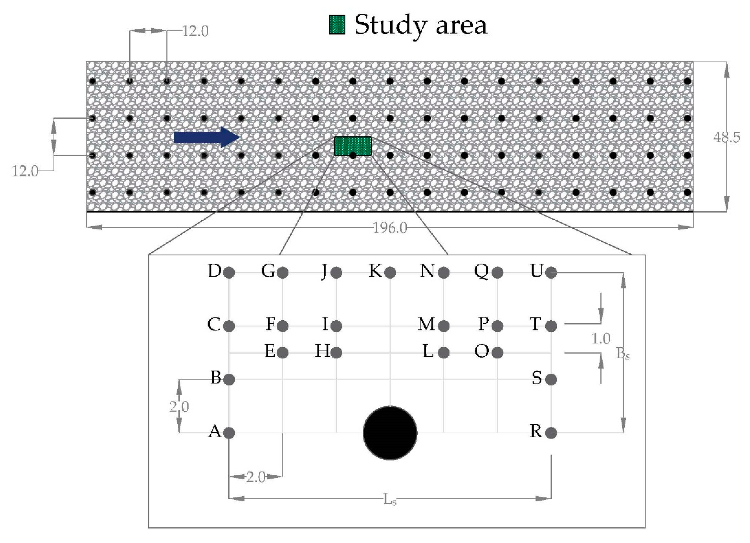
2. Experimental Set-Up

The experimental runs were carried out in a 9.6 m long, 0.485 m wide, and 0.5 m deep tilting flume at the Laboratorio “Grandi Modelli Idraulici” (GMI), Università della Calabria, Italy. The flume side walls are made of glass in order to visualize the flow. The inlet of the flume includes a stilling tank, an uphill slipway, and honeycombs (10 mm in diameter) in order to dampen the flow disturbances at the entrance. A downstream tailgate regulates the flow depth h inside the flume. All the runs were performed with h ≈ 0.14 m, which was measured 50 cm upstream to the vegetation array by a point gauge with a decimal Vernier (accuracy of 0.1 mm). The outflow is collected downstream in a tank equipped with a calibrated sharp-crested V notch weir to measure the flow discharge Q, which was set equal to 19.73 L/s, with a cross-section average flow velocity U of 0.30 m s⁻¹, where U = Q/(Bh), B being the flume width. A hydraulic jack was operated to set the bottom slope of the flume i_f at 1.5‰.

The vegetation array was simulated with vertical, rigid, and circular wooden cylinders, whose surface was made waterproof. The cylinder diameter and the height were d = 0.02 m and h_c = 0.40 m, respectively. Cylinders were inserted into a 1.96 m long, 0.485 m wide, and 0.015 m thick Plexiglas panel, which in turn was fixed to the channel bottom. Cylinders were arranged regularly with an axis-to-axis distance ΔS = 0.12 m in both the streamwise and spanwise directions (Figure 1). Therefore, the frontal area per canopy volume was a = d/ΔS² = 1.4 m⁻¹, while the solid volume fraction occupied by the canopy elements was ϕ = (π/4)ad = 0.02. Following Nepf [23], this vegetation can be considered as dense.

Three different bed roughness conditions were tested during the experimental campaign, employing very coarse sand (d₅₀ = 1.53 mm), fine gravel (d₅₀ = 6.49 mm), and coarse gravel (d₅₀ = 17.98 mm), respectively. In all the cases, the sediments were relatively uniform since the geometric standard deviation σ_g = (d₈₄/d₁₆)^0.5 was less than 1.5 [54], where d₁₆ and d₈₄ are the 16% and 84% (by weight) finer sizes of sediments, respectively. To prepare the bed, sediments were initially spread within the flume and screeded to create a bed with the same longitudinal slope of the channel. Figure 2 shows the laboratory flume after this preliminary phase, for each experimental run.

Table 1. Hydraulic parameters of the experimental runs for the approaching flow.

Parameter (Units)	Run 1	Run 2	Run 3
d50 (mm)	1.53	6.49	17.98
h (m)	0.137	0.137	0.136
Q (L/s)	19.73	19.73	19.73
U (m/s)	0.30	0.30	0.30
u* (m/s)	0.017	0.022	0.028
Uc (m/s)	0.46	0.75	1.05
if (‰)	1.50	1.50	1.50
T (°C)	21.70	21.44	20.80
ν (m2/s)	9.63 × 10−7	9.69 × 10−7	9.83 × 10−7
Fr	0.26	0.26	0.26
Re*	54	295	1024
Red	6231	6192	6104

shows the hydraulic characteristics of the experimental runs for the approaching flow, where u* is the shear velocity, U_c is the threshold flow velocity for the incipient sediment motion, T is the water temperature, measured with an integrated thermometer with an accuracy of 0.1 °C, and ν is the water kinematic viscosity, determined as a function of the water temperature [55]. Accurate estimation of the shear velocity can be achieved by extending the Reynolds stress distribution linearly to the roughness crest (e.g., [56]). Thus, the u* was estimated at the maximum sediment crest level, 50 cm upstream to the vegetation array, as ${\left(-\rho \overline{u^{\prime }{w}^{\prime }}/\rho \right)}^{0.5}$, where $\rho$ is the density of water, $u^{\prime }$ and $w^{\prime }$ are the temporal velocity fluctuations in the streamwise and vertical directions, respectively, and the symbol $\overline{·}$ indicates the time average. The flow velocity U_c was determined, still 50 cm upstream to the vegetation array, using Neill’s formula [57] as:

$$U_c=\sqrt{2.5{\left(\frac{h}{d_{50}}\right)}^{0.2}g\Delta d_{50}},$$

(1)

where g is the gravitational acceleration and Δ $=\left({\rho }_s-\rho \right)/\rho$ (where ${\rho }_s$ is the grain density) is the relative submerged grain density.

Furthermore, 50 cm upstream to the vegetation array, the flow Froude number Fr = U/(gh)^0.5, the Reynolds number of the sediments Re* = u*ε/ν (where ε is the equivalent sand roughness height, equal to about 2d₅₀) and the Reynolds number of the vegetation stems Re_d = Ud/ν were calculated. Note that the experimental runs were conducted in a clear-water condition, which was confirmed from the direct observation and from the flow condition that U < U_c.

3. Methodology and Reference Hydraulic Conditions

A down-looking acoustic Doppler velocimeter (ADV) probe (Nortek Vectrino), with an accuracy of 5% (assessed in previous works), installed on a motorized 3-axis traverse system (HR Wallingford), was used to measure the 3D instantaneous velocity components (streamwise u, spanwise v, and vertical w). The traverse system allowed an easy movement of the ADV probe in the study area during the experimental run with a spatial coordinate accuracy of 0.1 mm. The Vectrino transmitting length was 0.3 mm, and the sampling volume was a cylinder with a diameter of 6 mm and a height of 1 mm. The data acquisition was performed at a sampling frequency of F_s = 100 Hz over a period of 180 s, which was found to be adequate to have time-averaged velocities and turbulence quantities being statistically time-independent. The transmitted acoustic beams converged at 5 cm below the probe. Hence, the measurements were not feasible within the flow zone 5 cm below the free surface. This includes the free surface region, which is affected by the oscillations of the free surface [26]. Figure 3 shows the mean local water levels h_l measured within the study area for each experimental run. Owing to the free-surface waves, the water levels varied, both in space and in time, in the portion of the flume populated by the vegetation stems, and also around the single stem [45].

Prior to the use of the ADV data for the analysis, spikes were detected by the phase-space thresholding method and replaced by a third-order polynomial through 12 points on both sides of the spike, as suggested by Goring and Nikora [58].

For each experimental run, 21 vertical profiles were measured at the points shown in the x-y plane represented in Figure 1 and identified with the letters from A to U; z is the vertical axis above the maximum crest level in the study area. The vertical resolutions were 3 mm for $z\le 15 \mathrm{mm}$ and 5 mm above.

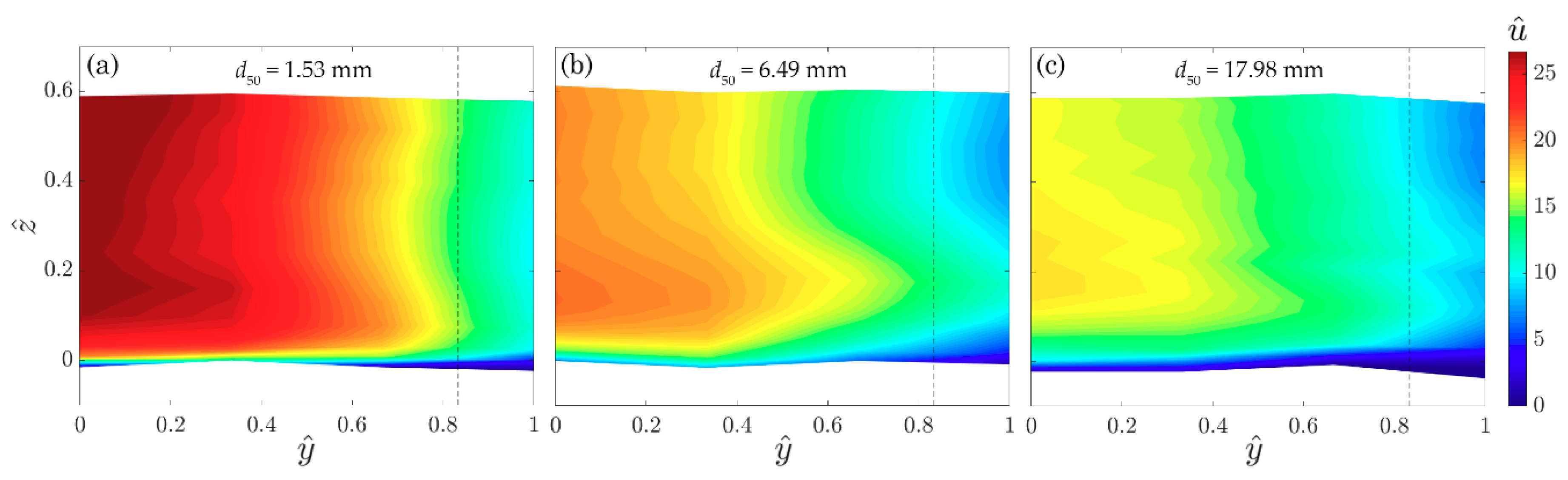
To characterize the undisturbed flow condition 50 cm upstream to the vegetation array, another vertical profile was measured at the flume centerline (y = 0) during each experimental run. Figure 4a shows the undisturbed vertical distributions of dimensionless time-averaged streamwise velocity $\widehat{u}$ $=\overline{u}/u_{*}$ (where $\overline{u}$ is the time-averaged streamwise velocity) for the three runs. The vertical axis, represented by $\widehat{z}$, was made dimensionless, dividing z by h_l. Note that for the undisturbed flow condition, the h_l coincides with the flow depth h reported in Table 1. As usually observed in an open-channel flow, the flow velocity u increases as the vertical distance z increases, and in the roughness sublayer (the flow layer where the effects of roughness elements are predominant), it tends to become zero owing to the bed roughness [56]. However, the most relevant aspect is the variation of $\widehat{u}$ between the three runs owing to the different bed roughness condition, which leads to an increase of the shear velocity (Table 1) and, therefore, to a decrease of $\widehat{u}$ as d₅₀ increases. The variation of the dimensionless Reynolds shear stress ${\widehat{\tau }}_{uw}$ $=-\overline{u^{\prime }{w}^{\prime }}/u_{*}^2$ and of the dimensionless viscous shear stress ${\widehat{\tau }}_{\nu }$ $=\nu \left(\mathrm{d}\overline{u}/\mathrm{d}z\right)/u_{*}^2$ along the vertical axis are depicted in Figure 4b,c, respectively. These latter are referred to the buffer layer, since the height of the ADV sampling volume did not allow measurements below 0.5 mm from the bed surface, where the viscous sublayer should lie. Specifically, the predominance of the Reynolds shear stress above the roughness sublayer can be observed; conversely, ${\widehat{\tau }}_{\nu }$ is negligible above the roughness sublayer, as the vertical distance z increases, with respect to ${\widehat{\tau }}_{uw}$. The viscous shear stress reaches the peak approximately at the maximum crest level for each experimental run. Instead, the Reynolds shear stress reaches the maximum value above the maximum crest level and then it diminishes as the vertical distance z increases.

The measured velocity data were analyzed through the second-order statistics of turbulence, that is the energy spectra E_u(f) of the velocity fluctuations. Here, f is the frequency, with a resolution defined as F_s/N, where N is the number of samples that, for a total duration of 180 s, equals 18,000. The estimation of energy spectra was carried out applying the discrete fast Fourier transform of the autocorrelation function. As an example, Figure 5 shows the energy spectra calculated for the three runs at two different elevations: Figure 5a refers to z = 0.05 h for the near-bed region, and Figure 5b to z = 0.4 h for the intermediate region.

The results were presented in terms of the wave number k, given by $k=2\pi f/\left[\overline{u}\left(z\right)\right]$, obtained by using the Taylor frozen-turbulence hypothesis [59]. Therefore, the wavenumber energy spectrum was estimated as $E_u\left(k\right)=E_u\left(f\right)·\left[\overline{u}\left(z\right)\right]/\left(2\pi \right)$ and it represents the contribution to TKE by wave numbers.

For both the intermediate and near-bed flow regions, for k ≤ 10 rad m⁻¹, associated with large scale, the spectral peaks are prominent, revealing the energy production range. Instead, the signals in the range 10 rad m⁻¹ ≤ k ≤ 2 × 10² rad m⁻¹ suggest the meso-scale motions [60]. Here, the inertial subrange is obtained, where the energy spectra follow a constant slope being in agreement with Kolmogorov’s 5/3-law. Furthermore, for k > 2 × 10² rad m⁻¹, the energy spectra indicate the presence of the so-called viscous-convective range, in which viscosity prevails on the diffusion [61]. This may be attributed to the concentration of the tracer used for the ADV measurements, which determined an increase in fluid viscosity at the expense of diffusion. In this case, the diffusivity becomes effective at much smaller scales than those at which viscosity prevails, which, however, cannot be detected at the ADV frequencies [62].

4. Time-Averaged Velocity, Reynolds Stress, and Viscous Stress

The contours of the dimensionless time-averaged streamwise velocities on the vertical central plane (identified with the letters from D to U in the streamwise direction) are shown in Figure 6 for each experimental run. Here, the horizontal axis, represented as $\widehat{x}$, was made non-dimensional by dividing x by the length of the study area (L_s = 12 cm), where x = 0 represents the streamwise location of the lateral plane where the vertical profiles A, B, C, and D were acquired. It is evident that the flow velocity increases with the vertical distance. However, a streamwise variation of the velocity field is detected. In the intermediate region below the free surface region ($z>0.1h_l$), the flow is strongly influenced by the vegetation. Specifically, in correspondence to the cylinder ($0.42L_s<x<0.59L_s$), $\widehat{u}$ increases with respect to the areas upstream to and downstream of the cylinder. This is a zone in which the flow converges, showing maximum velocity values [35]. These low/high velocity patterns are usually observed independently of the density and distribution of the vegetation elements [26]. A limited streamwise velocity variation is also visible in the roughness sublayer, in this case owing to the different bed features that characterize the three experimental runs.

The lateral variation of the dimensionless time-averaged streamwise velocities (vertical plane from D to A in the spanwise direction) is shown in Figure 7 for each experimental run. Here, the horizontal axis, represented as $\widehat{y}$, was made non-dimensional by dividing y by the width of the study area (B_s = 6 cm). It is possible to note a strong lateral variation of $\widehat{u}$ from the central plane (convergent flow) to the cylinder (divergent flow inducing the typical wake [35]). In correspondence to the cylinder ($0.83B_s<y<B_s$), referring to Run 1, the $\widehat{u}$-distribution assumes a quite constant value equal to 10, which indicates a reduction in the streamwise velocity of about 65% in the intermediate region and of 58% in the near-bed region. At the same location for Run 2, the reduction in $\overline{u}$ is of about 65% for $z>0.25h_l$, 50% for $0.1h_l<z<0.25h_l,$ and 61% for $z<0.1h_l$. Besides, for Run 3, the reduction in $\overline{u}$ is of about 55% for $z>0.35h_l$, 50% for $0.1h_l<z<0.35h_l,$ and 59% for $z<0.1h_l$. Therefore, in the intermediate region, the flow field is highly influenced by the vegetation regardless of the bed roughness. Moving toward the bed, the flow velocity is affected by both vegetation and bed roughness. As d₅₀ increases, this zone becomes more extended. However, in the near-bed flow, the flow field results to be still influenced by vegetation and bed roughness, with a predominance of this latter, owing to the interactions with the bed.

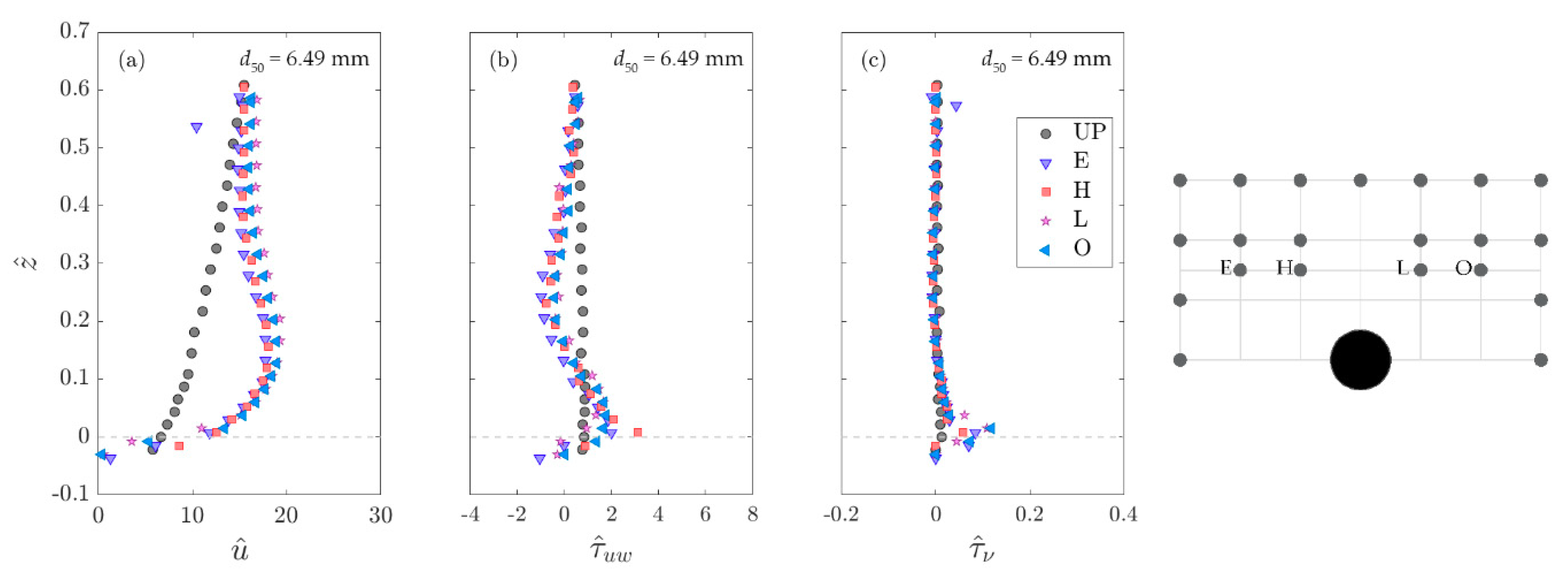
To examine the changes in the flow field induced by the presence of rigid vegetation, Figure 8, Figure 9, Figure 10, Figure 11, Figure 12, Figure 13, Figure 14, Figure 15 and Figure 16 show the vertical profiles of the (a) dimensionless time-averaged streamwise velocity component, (b) dimensionless Reynolds shear stress, and (c) dimensionless viscous shear stress, measured in the whole study area for each experimental run. Specifically, Figure 8, Figure 9 and Figure 10 refer to the vertical profiles measured at the flume centerline ($y=0$, that is 6 cm distant from the cylinder axis). Figure 11, Figure 12 and Figure 13 show the vertical profiles at $y=0.5B_s$, that is 3 cm far from the cylinder axis. Finally, the lateral variation of the vertical profiles is shown in Figure 14, Figure 15 and Figure 16, which correspond to the plane at $x=0$. Note that in Figure 8, Figure 9, Figure 10, Figure 11, Figure 12, Figure 13, Figure 14, Figure 15 and Figure 16, the profiles indicated as UP (undisturbed profile) correspond to the approaching flow measured at y = 0.

From the analysis of Figure 8a, Figure 9a and Figure 10a, it is evident that the presence of vegetation has a very noticeable effect on the velocity profiles at the flume centerline: it causes higher streamwise velocities than in the undisturbed flow conditions along the whole water depth. At each measurement location, the cylinders cause the velocity profile to collapse on a nearly vertical line (for $z>0.1h_l$). Here, the flow velocity is at least 1.2 to 2 times higher than that of the UP at $z=0.1h_l$. These results agree with those obtained by several researchers, including Liu et al. [53], Ricardo et al. [43], and De Serio et al. [35]. Approaching the bed, the influence of vegetation decreases and the streamwise velocities drop down toward zero, owing to the interaction with the bed. Specifically, the bed roughness causes a very large decrease in velocity (about 30–50%), which is higher for Run 3 than for Run 1. As regards the Reynolds shear stresses shown in Figure 8b, Figure 9b and Figure 10b, each profile measured at the flume centerline exhibits small and similar magnitudes in the region controlled by the vegetation. This behavior was already found by Ricardo et al. [43], who stated that the Reynolds shear stresses exhibit very small magnitudes, almost vanishing in the region controlled by the stems. However, near the bed, the roughness causes a pronounced peak in the vertical distribution. It is also evident that the maximum value of ${\widehat{\tau }}_{uw}$ is higher than that in the UP for each experimental run, but it is not influenced by the change in bed roughness, since ${\widehat{\tau }}_{uw}$ assumes a comparable value in all the runs. The viscous shear stresses do not reveal differences between the two cases (absence and presence of rigid vegetation) at the flume centerline, except for the reached maximum value, which is higher in the presence of vegetation (Figure 8c, Figure 9c and Figure 10c). Furthermore, as the roughness decreases, the viscous shear stress increases.

The spatial variation of the time-averaged velocity, Reynolds shear stress, and viscous shear stress profiles was investigated considering another longitudinal section (closer to the cylinder in the study area) and a lateral section (upstream to the cylinder).

In the immediate vicinity of the cylinder, the streamwise velocity decreases: it is lower than that measured along the centerline. Furthermore, analyzing the vertical distribution, $\widehat{u}$ reaches approximately the same intensity of that in the undisturbed condition in the upper part of the intermediate region ($z>0.5h_l$). This occurs in all the runs (Figure 11a, Figure 12a and Figure 13a), confirming the presence of a strong horizontal velocity gradient. However, for $0.1h_l<z<0.5h_l$, the velocity profile is again nearly vertical and, for $z<0.1h_l$, rapidly decreases, until becomes null owing to the interaction with the bed. Regarding both the Reynolds shear stress (Figure 11b, Figure 12b and Figure 13b) and the viscous shear stress (Figure 11c, Figure 12c and Figure 13c), they assume small values along the water depth, except for an increase in the vicinity of the bed. At the same time, it is noticeable that the maximum Reynolds shear stresses are lower than those measured at the centerline, highlighting a predominance of the effects induced by the vegetation on those related to the bed roughness in the vicinity of the cylinder.

Looking at the vertical distributions shown in Figure 14a, Figure 15a and Figure 16a, it is possible to note the increase of the streamwise velocity from A to D, that is from the point in line with the cylinders to the point laying on the flume centerline. Interestingly, for Run 1 at the point A, the velocity is always lower than that of the UP. This zone between two consecutive cylinders is characterized by a strong velocity reduction caused by the wake vortexes. However, for Runs 2 and 3, the velocity at the measurement point A is close to that of the UP for $z<0.15h_l$. This means that, as d₅₀ increases, the effect of the bed roughness is such as to control the near-bed flow, despite the presence of vegetation and the wake vortexes. Moving toward the flume centerline, this effect is added to that provoked by the vegetation, resulting in higher $\widehat{u}$ than those of the UP. In particular, at the point B, the velocity assumes similar values to those of the UP for $z>0.3h_l$. Furthermore, the differences between the profiles C and D (the furthest profiles from the vegetation stem) disappear for $z<0.15h_l$, indicating again the great influence of the bed roughness in the near-bed flow, at the expense of the vegetation effects. A limited lateral variation of the Reynolds shear stresses (Figure 14b, Figure 15b and Figure 16b) and of the viscous shear stresses (Figure 14c, Figure 15c and Figure 16c) is observed. This is confined in the near-bed region, owing to the bed roughness effects. Specifically, moving from the profile D to A, a decrease of the corresponding maximum values is found.

5. Energy Spectra

The estimation of energy spectra was carried out for the three experimental runs, at several elevations from the bed surface and different locations within the study area. Specifically, Figure 17 shows the energy spectra at the measurement points A and K for Runs 1, 2, and 3 at z = 0.05 h and 0.4 h, respectively.

Looking at Figure 17, in the intermediate region (z = 0.4 h), the two spectra referred to the measurement points A and K (Figure 17a–c) differ from those measured for the undisturbed profile in all the experimental runs. In fact, the macro-turbulence can be associated to k ≤ 3 × 10 rad m⁻¹ (for the UP this limit was k ≤ 10 rad m⁻¹). This is the region in which the vegetation stems have a predominant effect on the flow. The discrepancies are more evident between the UP and A signals, regardless of the bed roughness, since the point A lies between two consecutive cylinders in the region of wake vortexes. The inertial subrange is obtained for k > 3 × 10 rad m⁻¹, suggesting the presence of meso-scale turbulence.

In the near-bed flow region (z = 0.05 h), for Run 3 (Figure 17f) at low wave numbers (large scale), all spectra tend to the same constant values, indicating that macro-turbulence is governed by the bed roughness, regardless of the measurement point location within the study area. These spectral peaks are prominent for k ≤ 10 rad m⁻¹ at the measurement point K and k ≤ 10² rad m⁻¹ at the measurement point A. This implies that the energy production range is extended to smaller scales at point A than at point K, suggesting that the influence of the vegetation stems can be appreciated at small scales in the region of wake vortexes. The same trend is visible in Runs 1 and 2 (Figure 17d,e). Note that all the signals, also in the near-bed flow region, compare well with Kolmogorov’s 5/3 scaling law in the inertial subrange.

6. Turbulent Kinetic Energy (TKE)

The determination of the spatial variations of TKE is of great importance in the evaluation of the dispersion process that occurs in open-channel flows. The mechanical dispersion is the consequence of the time-averaged spatial fluctuations [63], which, in the presence of rigid emergent vegetation and bed roughness, may be influenced by both the stems and d₅₀ in the near-bed flow. The TKE can be written as follows:

$$\mathrm{TKE}=\frac{1}{2}\left(\overline{u^{\prime }{u}^{\prime }}+\overline{{\nu }^{\prime }{\nu }^{\prime }}+\overline{w^{\prime }{w}^{\prime }}\right),$$

(2)

where ${\nu }^{\prime }$ is the temporal velocity fluctuation in the spanwise direction.

The contours of the dimensionless TKE ($=TKE/u_{*}^2$) on the vertical central plane (identified with the letters from D to U in the streamwise direction) are shown in Figure 18 for each experimental run. High values of TKE are found below the maximum crest level and up to $z<0.05h_l$ in the near-bed flow zone, where the bed roughness provokes the turbulence. It implies that the velocity fluctuations get excited by the sediments, causing an enhanced turbulence level in the vicinity of the crests. However, it decreases gradually, moving upwards from $z>0.05h_l$ to $z<0.1h_l$, owing to the damping in $u^{\prime }$, ${\nu }^{\prime }$, and $w^{\prime }$. The TKE is somewhat spatially nonuniform for all the experimental runs. The possible reason is accredited to the randomly composed surface sediments [64]. For $z>0.1h_l$, a slight recovery of TKE occurs, this time owing to the vegetation effect. Furthermore, a feeble streamwise variation of the TKE is detected: in correspondence to the cylinder ($0.42L_s<x<0.59L_s$), the TKE increases with respect to the areas upstream to and downstream of the cylinder, being a zone in which the flow converges and subsequently diverges (similar results were obtained by De Serio et al. [35]).

The lateral variation of the dimensionless TKE (vertical plane from D to A in the spanwise direction) is shown in Figure 19 for each experimental run. The TKE values in this figure are associated to the same colorbar used in Figure 18 but with different extreme values, owing to the necessity of highlighting the spatial variation of the TKE in the vertical central plane. It is possible to note a strong lateral variation of TKE from the flume centerline to the cylinder. In fact, high values of TKE are found within the wake region, as a consequence of the distribution of $u^{\prime }$ and ${\nu }^{\prime }$, that are highest on the von Kármán vortex street. In essence, in correspondence to the cylinder ($0.83B_s<y<B_s$), in the intermediate region, the TKE is highly influenced by the vegetation regardless of the bed roughness. However, as d₅₀ increases, the zone in which the TKE is maximum moves toward the bed. It suggests that the TKE results are affected by both vegetation and bed roughness, causing an increase in the velocity fluctuations. In the near-bed flow, the TKE is still influenced by the vegetation and bed roughness, with a predominance of this latter, which reduces the effect induced by ${\nu }^{\prime }$.

7. Concluding Remarks

This study examines the bed roughness effects on the turbulence characteristics of flows through emergent rigid vegetation, performing three experimental runs with relatively uniform bed sediments (ranging from coarse sand to coarse gravel) and under the same hydraulic conditions. The experimental data were also compared to highlight the differences between the absence and the presence of vegetation. The principal findings are summarized next.

With reference to the time-averaged velocity field, in the intermediate region, the flow velocity is strongly influenced by the vegetation regardless of the bed roughness. Specifically, at the flume centerline, the streamwise velocity increases with respect to the areas upstream to and downstream of the vegetation stem. At the same time, a strong variation of the time-averaged streamwise velocity occurs laterally from the flume centerline to the vegetation stem. This causes a reduction in flow velocity of more than 50%. However, moving toward the bed, the flow velocity is affected by a combined effect of vegetation, firstly, and bed roughness, secondly. As d₅₀ increases, this zone becomes more extended. Furthermore, the presence of vegetation has a very noticeable effect on the velocity profiles at the flume centerline, since it causes higher streamwise velocities than in the undisturbed flow conditions along the whole water depth.

The behavior observed from the time-averaged streamwise velocity is confirmed by the shear stresses distributions, which reach their maximum values near the bed surface, owing to the bed roughness. The peak observed in the vertical distribution of the Reynolds shear stress is higher than that of the undisturbed conditions for each experimental run. At the same time, the viscous shear stresses do not reveal differences between the absence and presence of rigid vegetation at the flume centerline, except for the reached maximum value, which is higher in the presence of vegetation. As the bed roughness decreases, the viscous shear stress increases.

The analysis of the energy spectra of velocity fluctuations revealed that in the intermediate region the macro-turbulence is associated to smaller scales than those observed in the absence of vegetation. This is more evident in the region of wake vortexes. Instead, in the near-bed flow region, at low wave numbers (large scale), all spectra tend to the same constant values, indicating that the macro-turbulence is governed by the bed roughness, regardless of the measurement point location within the study area. However, in the region of wake vortexes, the macro-turbulence is extended at smaller scales, implying again the influence of the vegetation stems.

Finally, the analysis of the TKE revealed high values below the maximum crest level and in the near-bed flow zone in the streamwise direction. This implies that the velocity fluctuations get excited by the sediments, causing an enhanced turbulence level in the vicinity of the crests. Mowing toward the free surface, this effect vanishes, inducing a reduction in TKE. However, owing to the presence of vegetation, a slight recovery of TKE occurs. A strong lateral variation of TKE from the flume centerline to the cylinder in the intermediate region was found as a consequence of the distribution of the velocity fluctuations that are highest on the von Kármán vortex street.

Additional work is required to characterize the turbulence structures in the different flow layers, giving much more importance to the near-bed flow layer, being a zone influenced by both vegetation and bed roughness. For example, this can be addressed analyzing the degree of departure from the idealized isotropic turbulence, i.e., the turbulence anisotropy.