Article

Influence of Scour Development on Turbulent Flow Field in Front of a Bridge Pier

1
College of Transportation, Shandong University of Science and Technology, Qingdao 266590, China
2
School of Civil Engineering, Beijing Jiaotong University, Beijing 100044, China
3
National Engineering Laboratory of Port Hydraulic Construction Technology, Tianjin Research Institute of Water Transport Engineering, Tianjin 300456, China
*
Authors to whom correspondence should be addressed.
Water 2020, 12(9), 2370; https://doi.org/10.3390/w12092370
Submission received: 5 July 2020 / Revised: 21 August 2020 / Accepted: 21 August 2020 / Published: 24 August 2020
(This article belongs to the Section Hydraulics and Hydrodynamics)

Abstract

:
This study concerns the turbulent flow field influenced by the scour development around a bridge pier. The scour hole evolution as well as the temporal variation of scour depth around the pier were firstly analyzed. Subsequently, the flow fields in front of the pier at different instants during the scour process were measured using particle image velocimetry (PIV). It shows that the scour depth at the pier front exceeds that of the pier side at the later scouring stage. The temporal development of scour depth can be well predicted by a simple practical engineering model based on an exponential function with a change in the two adjustable coefficients. The flow field indicates that with the development of scour hole, the downward flow in front of the pier becomes more prominent, meanwhile the flow becomes more turbulent. The variation tendency for both velocities and turbulence intensities along the streamwise direction in front the pier shows similarity. The Reynolds shear stress generally increases with developing scour hole, and the region with large value enlarges and moves upstream of the scour hole.

1. Introduction

Local scour around bridge piers is resulted from the interaction of local flow field with riverbed sediment, which is one of concerned issues in hydraulic engineering [1]. The severe scour will undermine the structure and even give rise to the failure of bridge [2]. It is therefore essential to accurately estimate the scour depth around piers to guarantee the safety of bridges.
In the past several decades, numerous studies on pier scour have been conducted focusing on the equilibrium scour depth, that is the maximum scour depth when it reaches to the equilibrium state [3,4]. However, in reality, natural flood duration is usually far shorter than what is needed to reach the equilibrium scour depth [5]. Hence, in order to predict the scour depth reasonably and accurately from the viewpoints of both the safe and economical design of bridge pier, it is necessary to study and identify the variation of scour depth with time during the pier scouring process.
In engineering practice, simple models (e.g., empirical equations) are normally used to predict the scour process. Compared with large number of equations to predict the equilibrium scour depth, fewer predictive equations are available on the temporal variation of scour depth (see the review [6,7]). The widely-used predictor for the temporal scour depth is normally given by an exponential expression [7,8]. However, there are two empirical coefficients c1 and c2 included in the equations, of which the value is usually ad-hoc and needs to be further clearly determined based on a solid physical explanation. For example, Sumer and Fredsøe (2002) [7] simply used c1 = c2 = 1 for convenience. Simarro and Martin (2004) [9] noted that the value of c1 controls the scour rate, that is the curve of scour development is shifted to the left by increasing c1 [9]. The value of c2 is usually considered as a constant [9], while it can vary under different flow conditions. Cheng et al. (2016) [8] pointed out that c1 and c2 are dependent on sediment coarseness. Ben and Mossa (2020, 2006) [10,11] applied this exponential function into predicting the temporal scour evolution downstream of a sloped grade-control structure. They found that compared to the scour evolution at the initial and equilibrium phases, the scour evolution during the intermediate phase under different conditions shows different trend and specifically different value of the two empirical coefficients c1 and c2. This indicates that the scour evolution at the intermediate stage is more influenced by the structural and hydraulic conditions. In the current study, the two adjustable coefficients were thoroughly discussed from both theoretical and experimental points of view.
The pier scour is a time-dependent process, and the flow fields around the pier is correspondingly changed with time during the bed scouring process [12,13,14]. The presence of scour hole radically alters the turbulent flow field, and the hydrodynamic characteristics (e.g., bed shear stress and turbulence quantities) are strengthened, which induces further sediment transport and scour development around pier [15]. For instance, the horseshoe vortex as well as the turbulent energy are enhanced with the development of scour hole [16,17], indicating that the flow mechanism effected by the presence of scour hole is different from the flatbed cases without scour hole, which needs to be further explored to deepen the understanding of the pier scouring process. Recently, Ben et al. (2020) [18] experimentally investigate the flow field within the scour hole downstream of bed sills, and further obtain a new scaling of the equilibrium scour depth based on the phenomenological theory of turbulence. Their results also indicates that the in depth understanding of the flow and turbulence influenced by the scour hole is essential to improve the prediction of scour depth.
Particle image velocimetry (PIV) is a type of non-intrusive velocity measurement technique which is capable of measuring the instantaneous velocity field in the defined flow region. Some scholars have utilized PIV to study the flow field for the pier on the fixed flatbed, e.g., Lin et al. (2003) [19], Huang et al. (2014, 2018) [20,21], Schanderl et al. (2014) [22], Ozturk et al. (2007) [23]. Recently, Li et al. (2018) [24] used the high-resolution PIV system to study the flow characteristics induced by the horseshoe vortex in front of the pier. Similar experimental studies can be found by Chen et al. (2019) [25] who systematically analyzed the transient evolution process of horseshoe vortex. The previous relevant PIV studies are mainly confined on the flow of a pier mounted on a flatbed without scour hole, which can be regarded as the initial scour state. The limited and valuable study on the flow affected by the pier scour hole can be found from Unger and Hager (2007) [26] who investigated the temporal evolution of the vertical deflected flow in front of the pier with increasing scour hole by PIV. Overall, the study on the flow field influenced by the development of scour hole at a pier by the high-resolution PIV measurement is rather limited so far.
To our knowledge, a comprehensive understanding of the flow field around piers affected by the scour development is still deficient. The purpose of the present study is twofold: (1) Obtain a simple practical model to predict the temporal scour depth; and (2) study the effect of scour development on turbulent flow field based on a high-resolution PIV system. The paper is organized as follows: The experimental setup and PIV measurement are described in Section 2. In Section 3 we discuss the scour development around the pier, involving the scour hole evolution and the temporal variation of scour depth, and a simple practical model to predict the temporal scour depth is developed and validated. In Section 4 the turbulent flow fields in front of the pier were investigated in terms of the time-averaged velocities, turbulence intensities, Reynolds shear stress and turbulent kinetic energy. Finally, summary and conclusions are drawn in Section 5. The present experimental results provide not only new insight into the complex flow fields around piers but also valuable experimental data to validate and verify numerical models.

2. Experimental Setup and Methodology

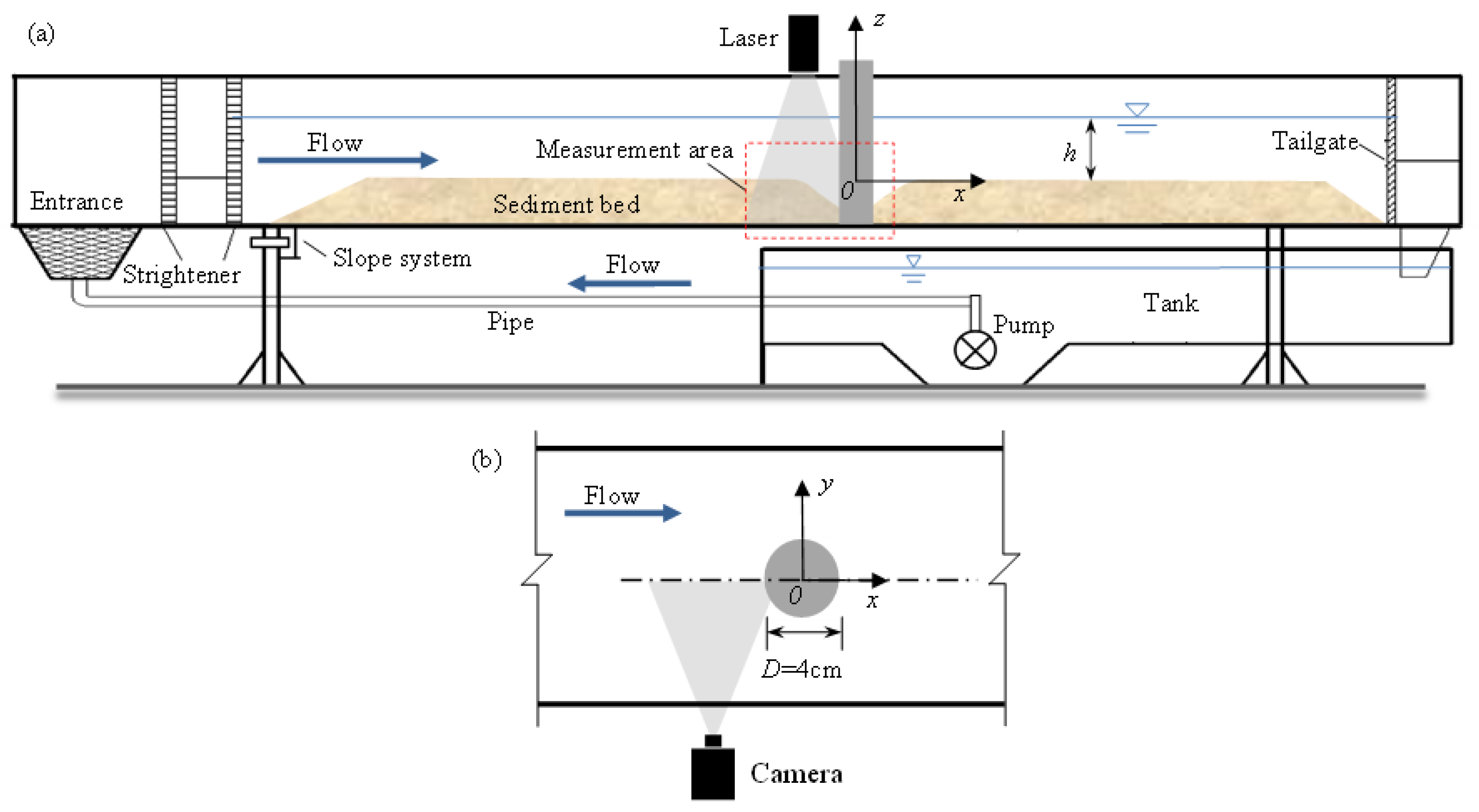
The present experiment was conducted in a water-recirculating and glass-walled flume with 6 m length, 0.25 m width and 0.25 m depth, at Bejing Jiaotong University. The Flow straightener was set at the entrance of the flume to calm the turbulence of flow, and a tailgate was set at the outlet of the flume to adjust the water depth. As depicted in Figure 1, a circular cylinder with diameter D = 4 cm was used to model the bridge pier, and mounted vertically on the bed at 4 m downstream of the flume entrance to ensure the fully developed flow occurred [27]. The sediment bed was set up on the bottom with median diameter d50 = 0.6 mm and specific mass ρs = 2650 kg/m3. The blockage ratio (i.e., flume width to pier diameter) in the present test is 6.25, which is in the proposed acceptable range [12,28,29]. The origin of the coordinate system is defined at the bottom center of the cylinder, with the longitudinal x-axis parallel to the flume bed, the y-axis normal to the side wall of the flume, and the z-axis vertical to the flume bottom.
The experiment was performed under a steady-flow condition, i.e., the incoming discharge from the inlet of the flume is constant. The flow depth h = 5 cm and the approaching depth-averaged flow velocity U0 = 0.233 m/s, the Reynolds number based on pier diameter (ReD) was 9400, and the Froude number based on water depth (Fr) was 0.28. The present Shields number was calculated as Θ0 = u2/[(ρs − ρ)/ρ]gd50 = 0.029, where u (=0.016 m/s) is the bed friction velocity obtained from the best fitting of a log-law profile of the approaching velocity, and ρ is the fluid density. In this test, the critical Shields number for incipient sediment motion on flat planar bed Θcr can be determined by the well-known diagram of Shields curve. Here, for convenience, Θcr = 0.033 is given by the method outlined in Soulsby and Whitehouse [30], and thus the test was performed in a clear-water scour condition (i.e., Θ0 < Θcr).
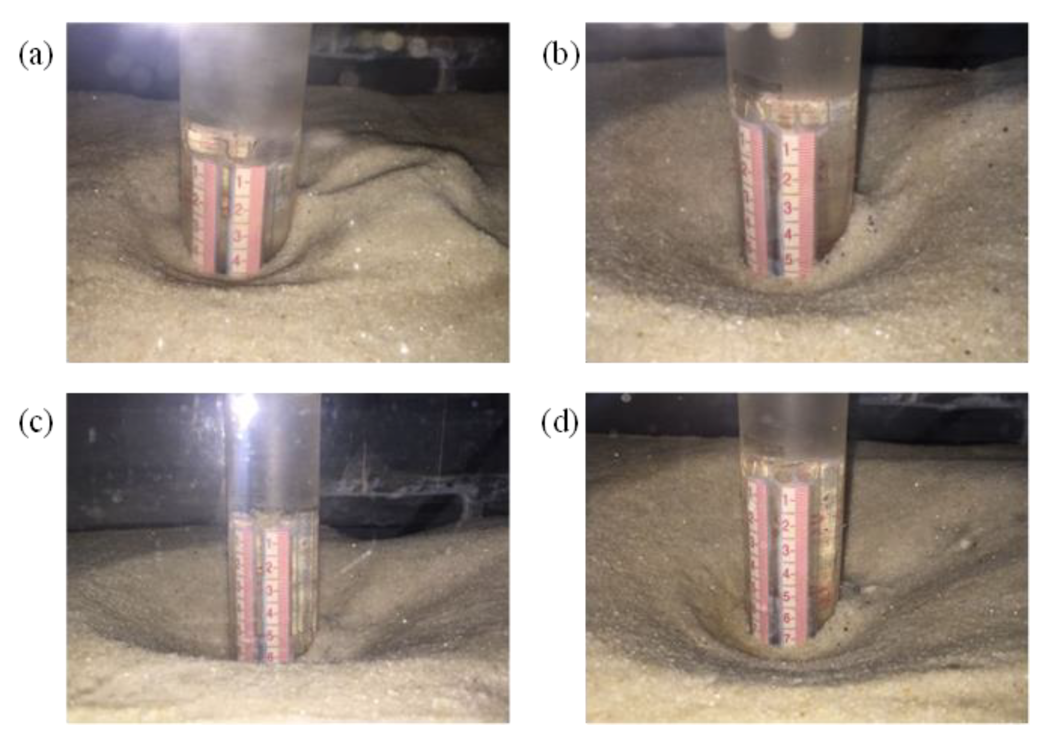
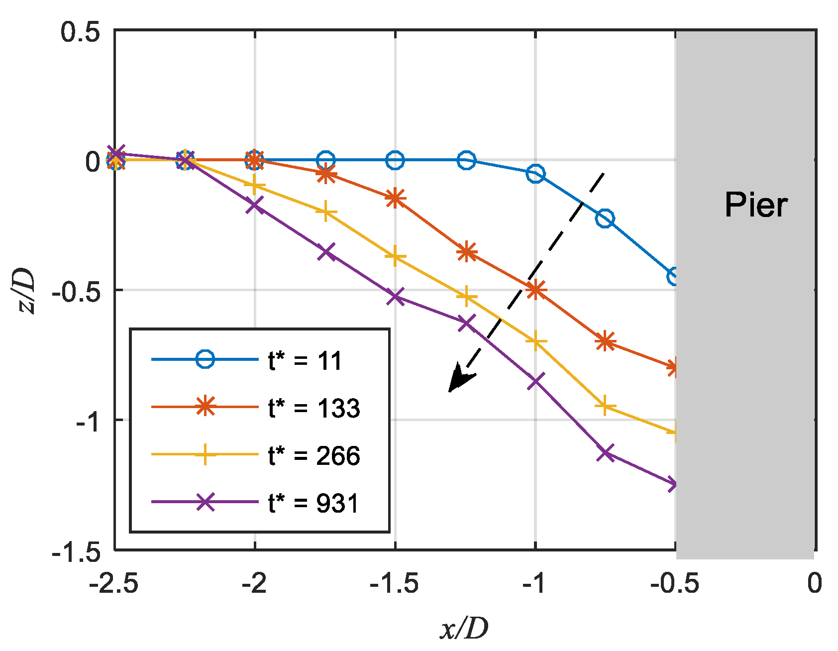
During the scouring process, the temporal variation of scour depth around the pier has been measured. A scale label was marked on the surface of the pier to facilitate the direct observation of the scour depths. The scour hole morphology was measured by a bed profiler, with space resolution of 2 mm. Since the geometry of the scour hole was observed symmetric about the symmetry plane of the pier, only half of the scour hole was measured.
The two-dimensional instantaneous flow fields in the symmetry plane in front of the pier were measured using a time-resolved PIV system, which consists of a high-speed camera, a pulse laser, tracer particles and post-processing software. It is worth noting that the scour holes that typically develop are, in fact, reasonably symmetric about the symmetry plane, and thus the time-averaged flow field on the symmetry plane can be regarded as two-dimensional in principle. The laser was placed directly above the flume and produced a 1 mm-thick light sheet illuminating the field of view. In order to perform PIV measurements, the flow was seeded with micro-spheres with mean diameters of 10 μm and specific gravity of 1.06. A high-speed digital CMOS camera with a Nikkor AF 50 mm f/1.4D lens was placed on one side of the flume to capture the high-resolution particle images. The camera has a maximum frame rate of 500 fps at full spatial resolution of 1280 × 1024 pixels, and the exposure time between two consecutive frames is 2 ms. The size of the camera viewing area is 52 × 42 mm such that the spatial resolution is 24.5 pixels/mm. Due to the limited memory of camera (2 GB), a sequence of 2000 frames was captured for each case, and we used 2000 frames to calculate the time-averaged flow field. It should be noted that since the cameras were positioned parallel to the test section and due to the presence of the sand bed, the field of view of the cameras was blocked. Hence, the measurements inside the scour hole greater than 1 cm could not be acquired.
The solution of instantaneous velocity vectors between two consecutive frames was achieved by using the iterative multigrid image deformation algorithm [31]. For the present application, the final interrogation window size was 32 × 32 pixels which have an overlap of 50%, that is the adjacent velocity vector interval is 16 pixels. Based on the flow velocity in our experiment, the interval time of 2 ms assured that the maximum particle displacement between two consecutive frames is 5 pixels, which satisfies the one-quarter rule for PIV correlation analysis [32,33]. The accuracy of the velocity vectors is approximately 0.1 pixels, which corresponds to approximately 0.7% of the full-scale velocity in the present measurement. For more specific details on the PIV setup, the readers can refer the previously published paper by the authors [24,
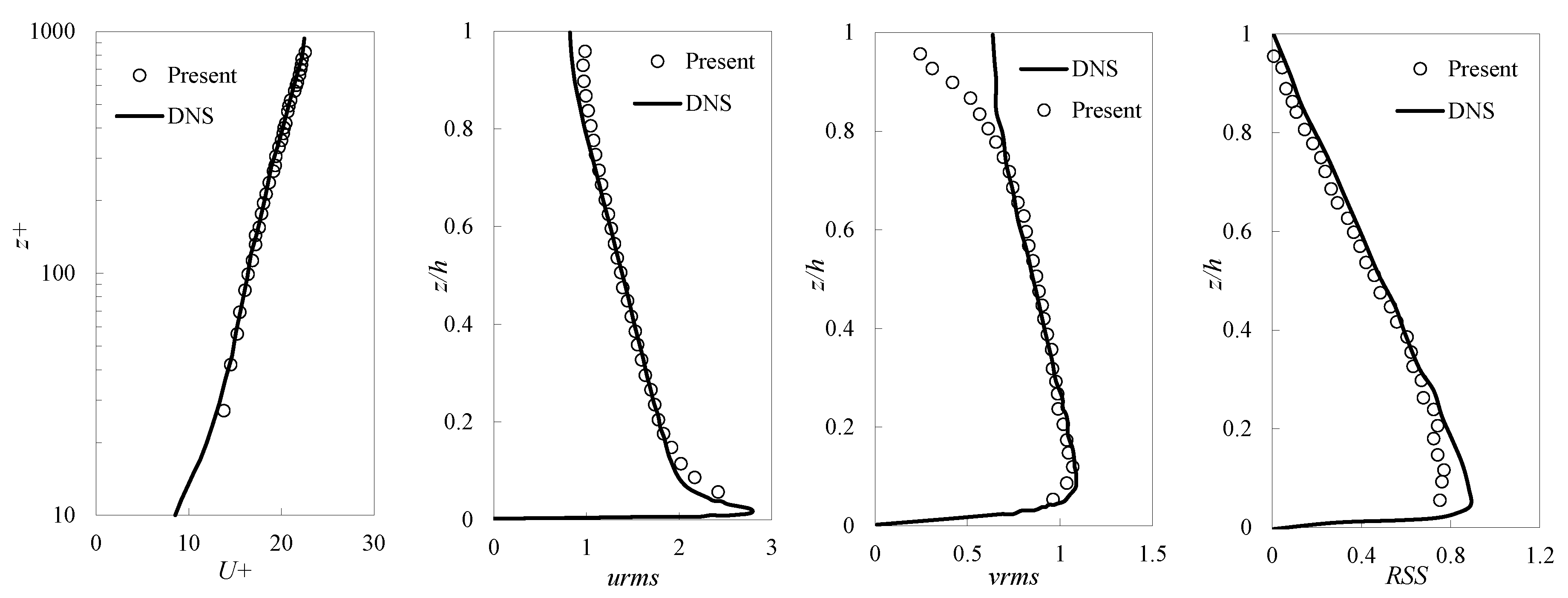
34]. The validation of the PIV measurement can be seen as the Appendix A.

3. Scour Development Around the Pier

3.1. Scour Hole Evolution

Figure 2 presents the photographs of local scour hole around the pier at four different instants during the scour process. In the figure, the approaching flow is from the left to right. The time t is normalized by:
t * = g ( s 1 ) d 50 3 D 2 t
As can be seen from the scale label on the pier surface, the scour hole around the pier becomes larger (i.e., deeper and broader) gradually with time, and eventually the equilibrium scour is almost attained. In fact, the duration to reach equilibrium in the laboratory can be very long, usually 1–2 weeks [35]. Hence, the present scour experiment with duration of 420 min is far shorter to reach the equilibrium. However, it can be seen from the experimental observation that the scour depth seems to be gradually approaching the equilibrium as the variation of scour depth at later stage is small and the scouring process is very slow with time. Hence it can be regarded as a quasi-equilibrium scour state. Here some of the characteristic features of the steady current scour around a pier can be observed. Upstream of the pier the expected semicircular shape of the scour hole is clearly visible, whereas the shape of scour hole downstream cannot be characterized as semicircular. Additionally, the scour depth behind the pier is obviously smaller than the scour depth in front of the pier, and downstream of the pier bed material is deposited along the edges of the scour. In the present study, we mainly focus on the region in front of the pier where the maximum scour depth is normally occurred and the influence of turbulent horseshoe vortex is most pronounced [24].
Figure 3 shows the scour morphology around the pier at different time of the scour process, in which the scoured bed elevation is normalized by the pier diameter D. As the scour profile is symmetrical along the spanwise (y−) direction, only half of region is plotted. It clearly illustrates the evolution of the scour hole around the pier, both the scour depth and scour area become larger with time. The maximum scour depth at the final equilibrium stage is located at the front of the pier. Furthermore, the evolution of scour profile along the centerline in front of the pier is specifically plotted in Figure 4. It can be seen that the bed slope at different time keeps almost same, which is approximately equal to the angle of repose. This visible finding is consistent with the previous studies [36,37].

3.2. Temporal Development of Scour Depth

The measured time series of the scour depth taken at both the front and back face of the pier are plotted in Figure 5. As can be seen, at the early stage, the scour depth at the side of the pier is clearly larger than that of the front of the pier, and the scouring rate is comparatively higher. At the later scouring stage, the scour depth at the front of the pier exceeds that of the pier side, and the final maximum scour depth occurs at the pier front. In fact, it is observed that scour starts from the sides of the pier due to the separation of flow creating a large amplification of bed shear stress at the side of the pier. As the scour develops with time, the bed shear stress at the side of the pier is decreased and the scour mechanism is mainly related to the turbulent horseshoe vortex at the pier front rather than the contracted streamlines, which results in the maximum scour depth occurred at the front position of the pier.
In engineering practice, simple models (e.g., empirical equations) are normally used to predict the scour process. The widely-used predictor for the temporal development of the scour depth is given by the following exponential expression [9]:
S S e = 1 exp [ c 1 ( t T s ) c 2 ]
where S is the scour depth, Se is the equilibrium scour depth, c1 and c2 are fitting coefficients which can be determined by the experimental data, and Ts is the time scale of scour calculated by integrating the scour curve [38]:
T s = 0 t m S m S S m d t
where Sm is the maximum scour depth at any given time and tm is the time at which the maximum scour occurs.
Figure 6 provides the comparison between the predicted and measured temporal development of scour depth at the side and front faces of the pier. For comparison, the predicted results by the equations with c1 = c2 = 1 (Sumer and Fredsøe, 2002) [7] and the current fitted value are both included in Figure 6. It clearly indicates that the results predicted by the current equation (blue solid line) with adjustable c1 and c2 fit better. The equation of Sumer and Fredsøe (2002) [7] under-predicts the scour depth during the early stage at which the scour rate is very high, especially for the side position of the pier. By inspection of Equation (1), when t is small, c1 represents the slope of the function which means the scour rate. Therefore, to improve the fitting degree with experimental data at the early scour stage, the value of c1 should be increased larger than 1 to increase the scour rate at the initial stage. As for the exponent c2, it characterizes the dependence of the scour hole volume (V) on the scour depth (S) from the physical meaning of pier scour, and c2 = 1/3 if the rate of change of V is the same as that of S3 [8]. Combining the above-mentioned analysis on the scour hole evolution, the scour hole deepens meanwhile extends horizontally, and the slope of the scour hole remains almost constant. If the scour hole is idealized and can be assumed as an inverted pyramid, then S is proportional to V1/3, and thus the exponent c2 is equal to 1/3, which is consistent to the value of 0.33 proposed by Simarro and Martin (2004) [9]. Based on the present experimental data, the value of c2 is smaller than 1, especially for the c2 at the side of the pier is 0.329, which is very close to the theoretical value of 1/3.
In order to further validate the simple predictive model proposed above, other previously experimental data from literature is collected [6,39,40], and the comparisons are plotted in the Figure 7 and Figure 8. In these experiments, the test duration for a single run lasted longer than 40 h, which is much longer than those reported in many other studies. The detailed experimental conditions for those tests are listed in the Table 1. Figure 7 presents the comparison of temporal scour depth at the pier front, in which the subplots (a)–(j) correspond to Test 1–10 listed in Table 1. The value of the two empirical constants c1 and c2 included in the exponential equation is given by the present proposed value, i.e., 1.046 and 0.510, respectively. It demonstrates that the present simple model fit well with the experimental data from other previous studies. Apart from the scour depth at the pier front which is always concerned, the scour depth at the pier side is also compared as plotted in Figure 8, for which the predicted results are based on c1 = 1.243 and c2 = 0.329. As can be seen, the present simple model does a good job of predicting the scour depth observed at both pier front and side. It needs to be noted that the limitation of our present study is only based on the experiments listed in Table 1, which is also the application condition for the current proposed model.

4. Turbulent Flow Fields

To identify the physics of the flow disturbed by the generation of the scour hole around the pier, the flow and turbulence characteristics at different scour stages (t* = 2, 11, 133, 266, 931) were analyzed and presented in this section. The flow fields at the symmetry plane in front of the pier were obtained as well as the typical flow and turbulence characteristics are described in detail, in terms of the time-averaged velocities, turbulence intensities, Reynolds shear stress, and turbulent kinetic energy. Moreover, the space-averaged quantities (can be regarded as the representative of the focused area) were obtained to clarify the influence of scour development on the flow and turbulence characteristics.
The instantaneous velocity components were denoted as u for the streamwise and v for the vertical direction along the x- and z-axes, respectively. Such instantaneous flow velocities could be separated into time-averaged (U, V) and fluctuating (u’, v’) components according to Reynolds decomposition (i.e., u = U + u’). The time-averaged velocity is obtained by averaging the instantaneous velocity. The streamwise and vertical turbulence intensities are calculated by urms ( = u 2 ¯ ) and vrms ( = v 2 ¯ ), respectively. The Reynolds shear stress (RSS) is calculated as RSS = ρ u v ¯ , and the turbulent kinetic energy (TKE) is calculated as TKE = 0.65 ( u 2 ¯ + v 2 ¯ ) [41].

4.1. Time-Averaged Velocities

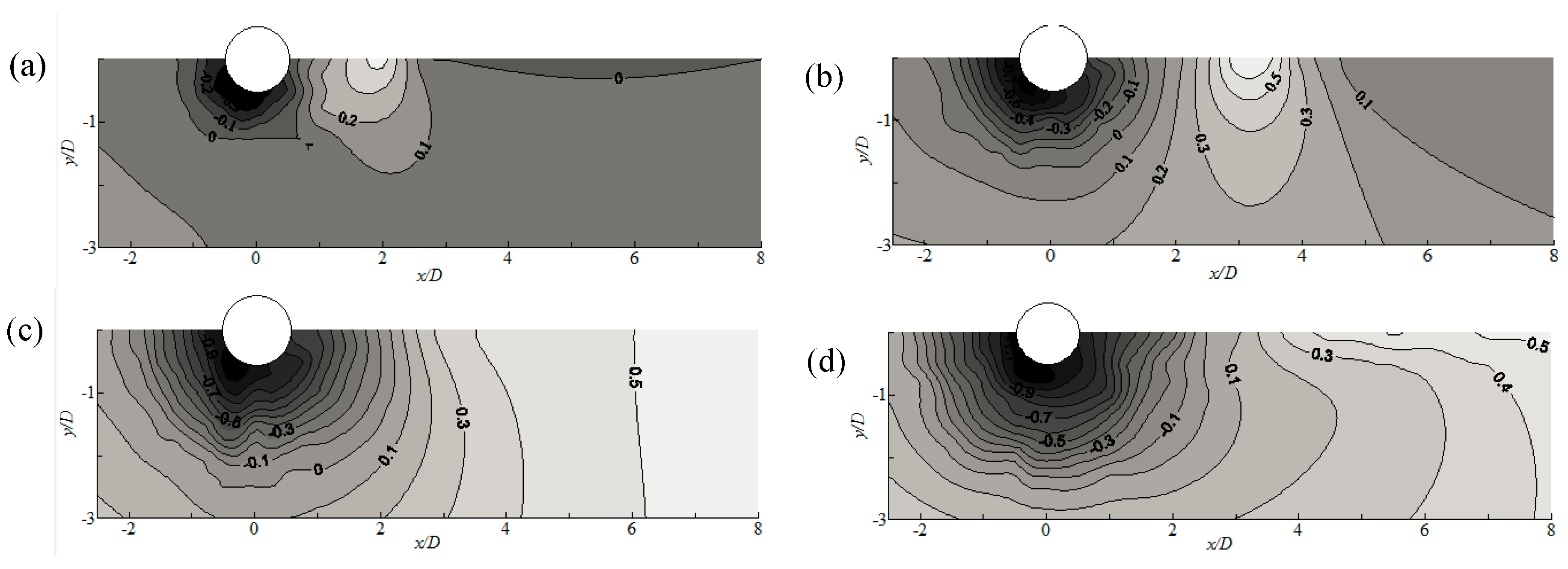
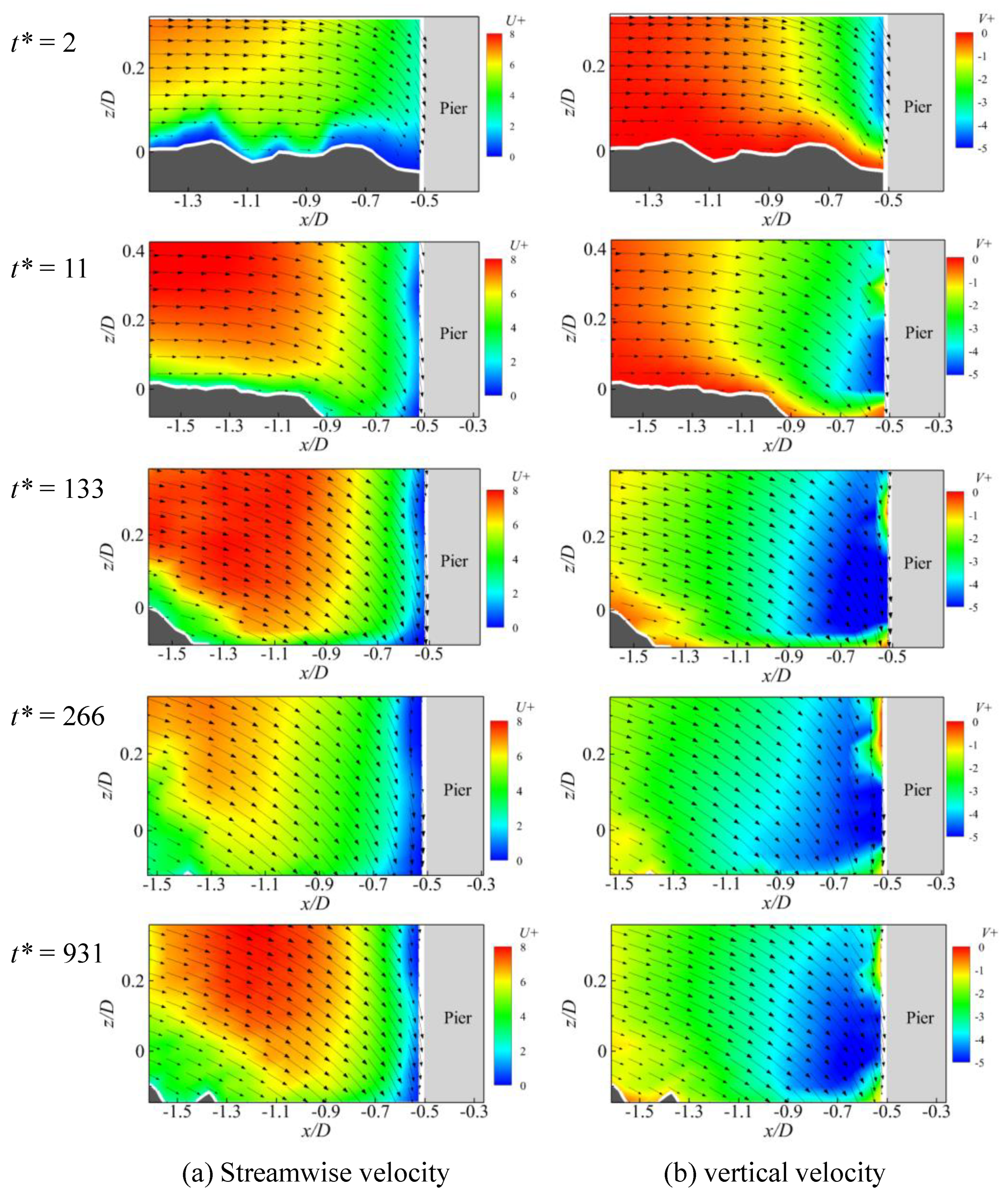
Figure 9 shows the velocity vectors superimposed on the velocity contours at different time during the scouring process. The velocity components, including the streamwise and vertical velocities are made non-dimensional with the friction velocity (U+ = U/u*, V+ = V/u*). It is worth noting that the results within the scour hole (i.e., below the initial bed) was not available because the sand bed at the lateral side blocks the optical access of the field view inside the scour hole. The vectors clearly illustrate the downward movement of flow (downflow) in front of the pier, and the downflow is more visible with the scour hole development. The streamwise velocity decreases when flow approaching to the pier due to its blocking effect. The contours of V+ show that the area with negative value of V+ in front of the pier expands, indicating that the downflow extends with developing scour hole. Moreover, the region with large value of V+ moves downward along the vertical direction as the scour depth increases.
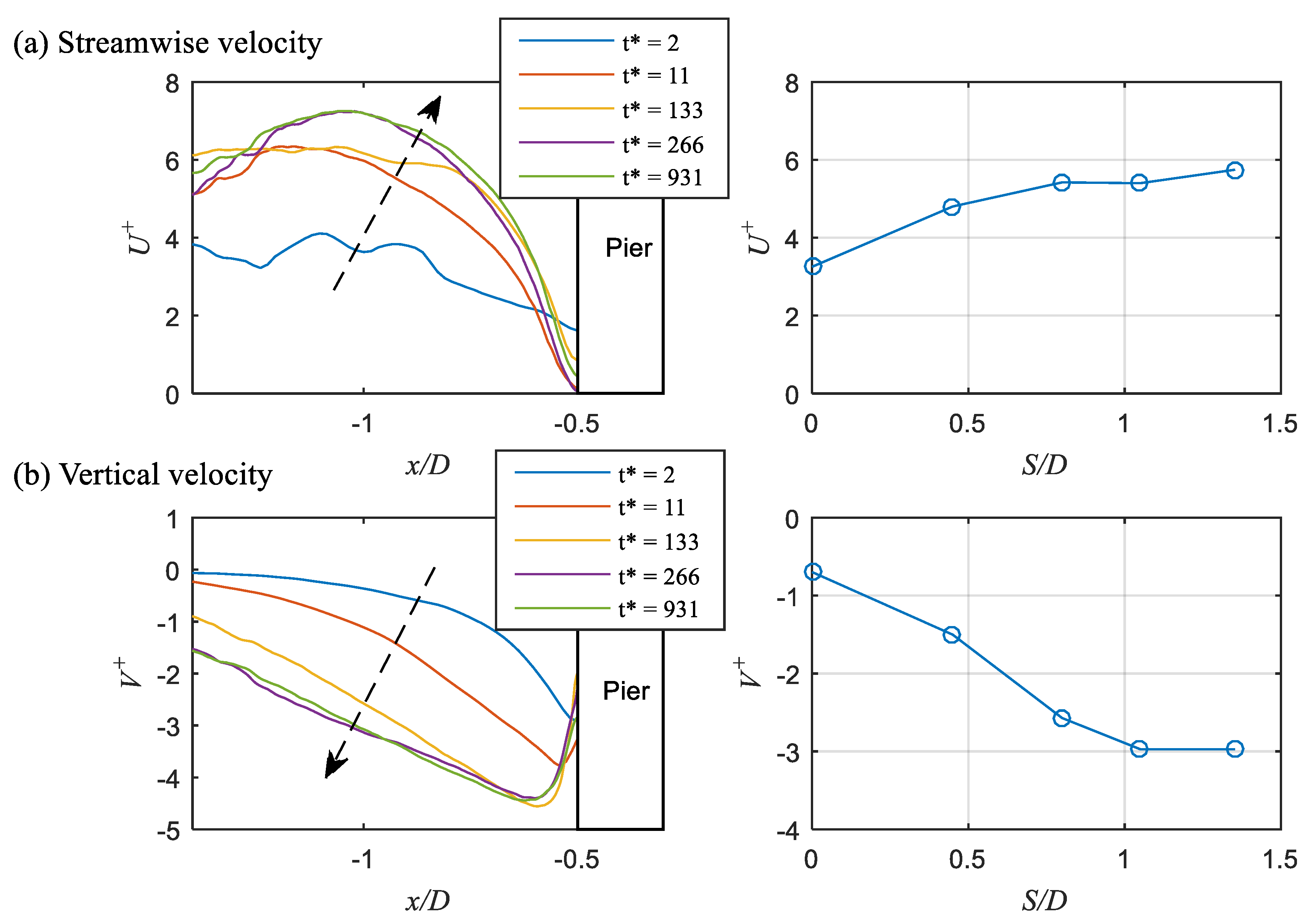
To further compare the variation of velocity under different scour depth, the space-averaged velocities were obtained and plotted in Figure 10. The left subplot is the velocity variation along the center line for which the value was obtained by averaging the velocities over vertical direction. To clearly show the influence of scoured bed on the velocity, the corresponding space-averaged results (i.e., by averaging the data in the measured area) versus scour depth were presented in the right subplot. That can be regarded as the double-averaged results obtained by both time and space averaging the instantaneous flow field data. The distribution of U+ (Figure 10a) along x direction exhibits that it is reduced significantly close to the upstream face of the pier. The magnitude of U+ generally increases with increasing scour depth. This can be explained that as the scour evolves upstream, the bed slope increases due to the formation of the scour hole, and the flow velocity is correspondingly increased. Figure 10b indicates that the value of negative V+ increases near the pier due to the formation of downflow, and the magnitude of V+ increases with increasing scour depth, especially for the early scouring stage with high scour rate. Combining the velocity contour analyzed above, it further indicates that with the increase of scour depth the downflow in front of the pier becomes more prominent, and both the extent and strength of the downflow increase with the development of scour hole. This finding is consistent with the results from the acoustic Doppler velocimeter (ADV) measurement by Dey and Raikar (2007) [12].

4.2. Turbulence Intensities

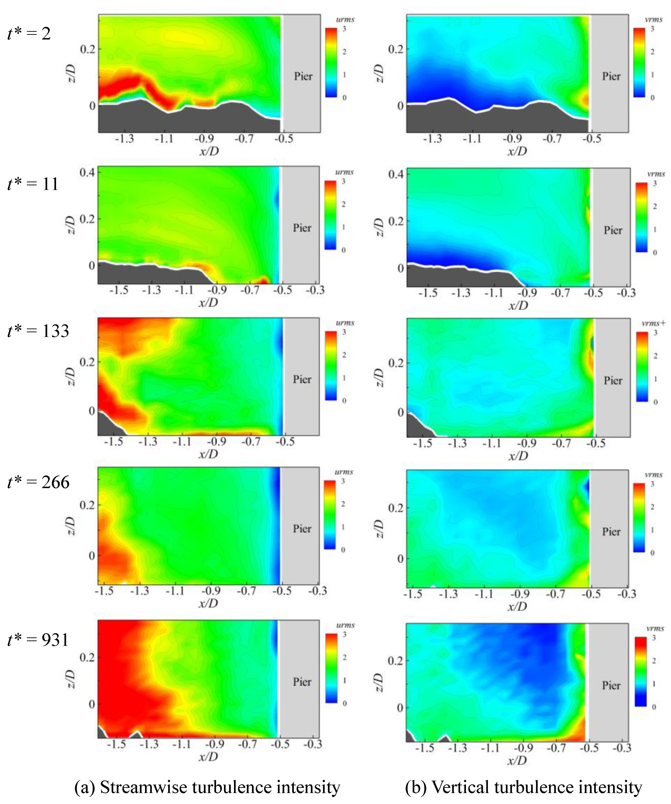
The contours of turbulence intensities at different time during the pier scouring process are depicted as Figure 11, in which the streamwise and vertical turbulence intensities (urms and vrms) are normalized by the friction velocity. Figure 11a shows that at the initial scour stage (e.g., t* = 2) the region with high value of urms is near the bed outside of the scour hole. With the development of scour, the region with large urms moves towards the inside of the scour hole meanwhile the extent with large urms becomes more significant. This is related to the horseshoe vortex within the scour hole, which was also observed by Dey and Raikar (2007) [12]. As the scour hole size increases, the strength and size of the horseshoe vortex increase, resulting in the associated turbulence intensity increases correspondingly. Figure 11b shows that the maximum value of vrms is located close to the upstream face of the pier, which can be further illustrated by the following Figure 12.
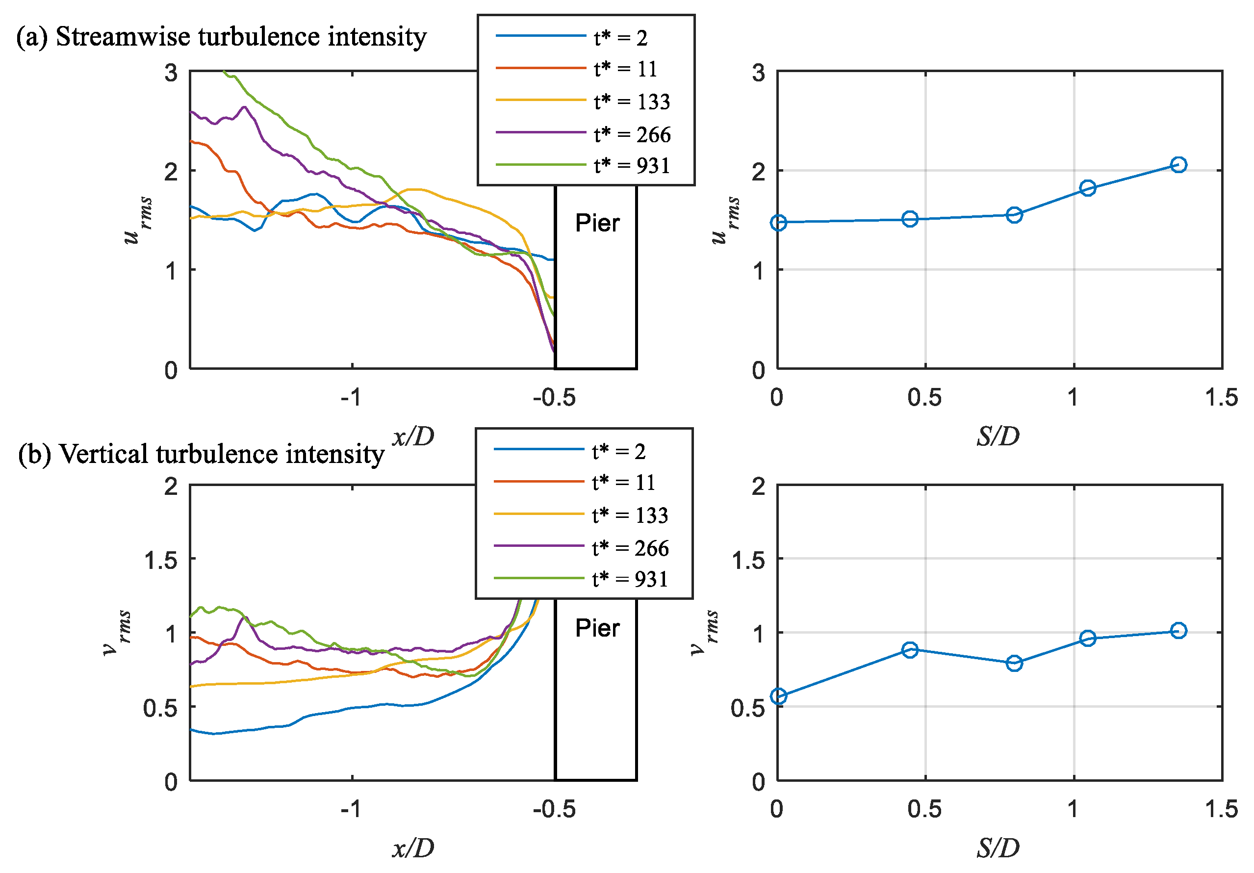
Figure 12 presents the distributions of turbulence intensities along the center line at different time during the pier scouring process, and the corresponding space-averaged value versus dimensionless pier scour depth is also plotted in the right subplot. It can be seen that the streamwise turbulence intensity is decreased close to the pier, while the vertical turbulence intensity is increased and reached the maximum just near the upstream face of the pier. This variation tendency is reasonably similar to the distribution of flow velocity as shown in the left subplot of Figure 10. The space-averaged value for both urms and vrms increase with increasing scour depth, and vrms is comparatively smaller than urms. Overall, the flow in front of the pier becomes more turbulent with the development of scour due to the effect of horseshoe vortex. This implies that the influence of turbulence on sediment transport becomes more prominent, which should be considered in the numerical computation of pier scour [24].

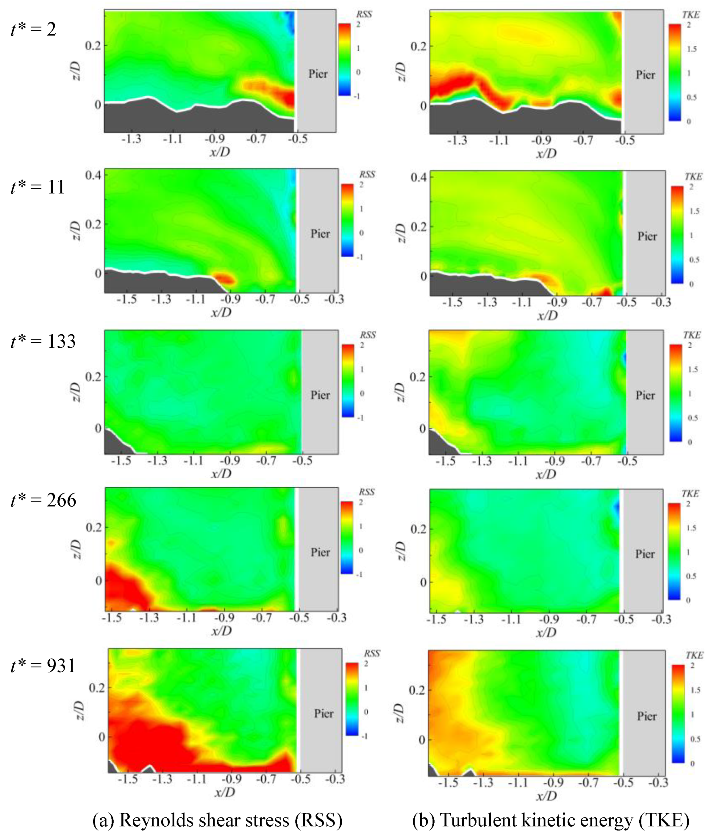
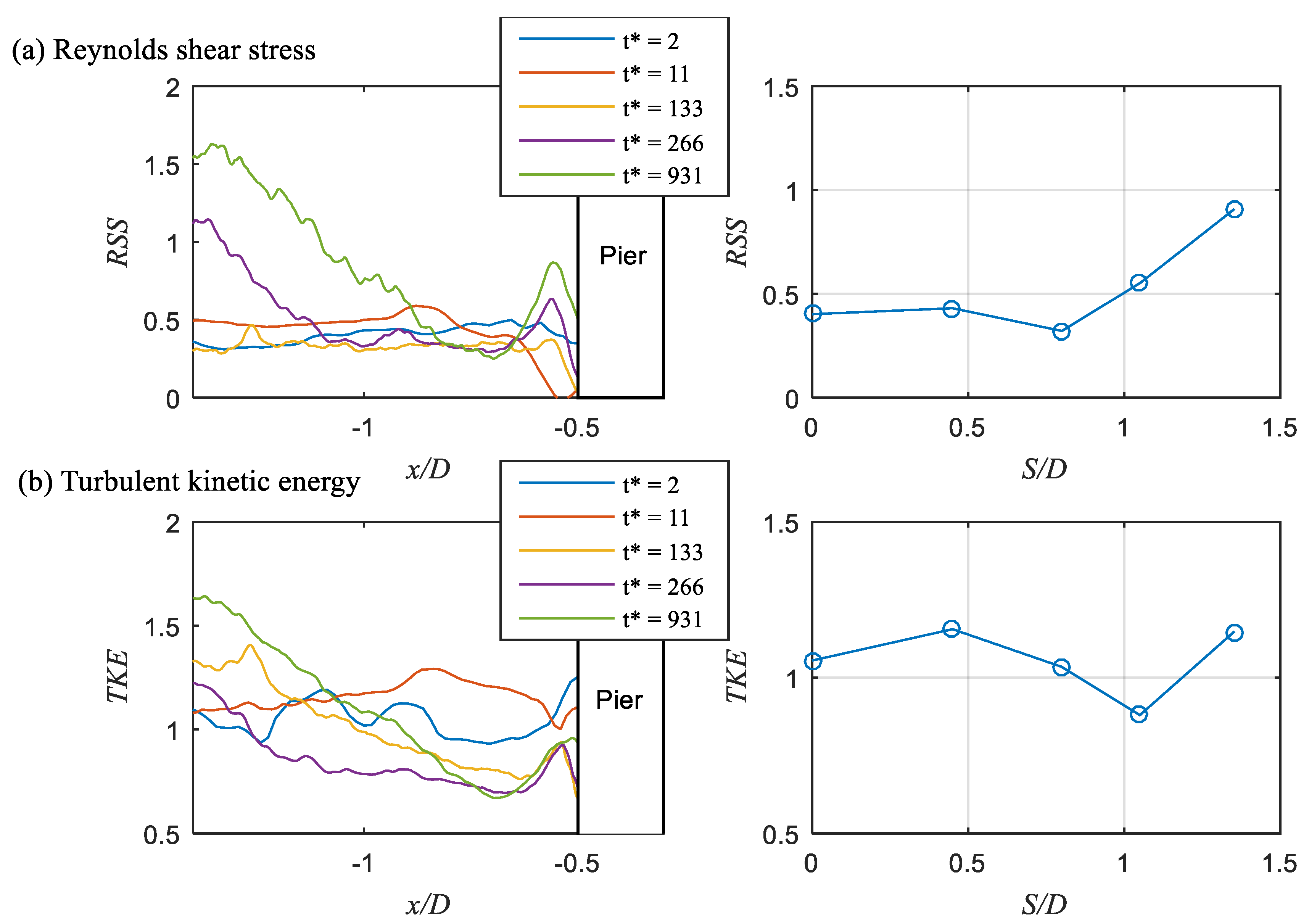
4.3. Reynolds Shear Stress and Turbulent Kinetic Energy

Figure 13 presents the contours of Reynolds shear stress (RSS) and turbulent kinetic energy (TKE) at different scour stage, in which the value is normalized by the friction velocity. It indicates that the region with large RSS expands with the scour hole development. For instance, the core of the high RSS is located at just the front of the pier at the initial scour stage (t* = 2). When t* = 11, the maximum RSS is occurred at the upstream edge of the scour hole (turning point) as a result of flow separation. As the scour evolves upstream, the flow with high RSS expands to the outside of the scour hole (e.g., see the red-color region at t* = 931), which is probably due to the effect of turbulent horseshoe vortex in the scour hole. The distribution of TKE is similar to that of streamwise turbulence intensity, which is consistent with the results of Dey and Raikar (2007) [12].
Figure 14 further illustrates the RSS increase with developing scour hole, and the large value of RSS enlarges and moves upstream as shown in the right subplot of Figure 14a. The variation of TKE with scour depth is relatively complicated rather than monotonic increasing or decreasing. It is inferred that the TKE is closely generated by the horseshoe vortex. With the development of scour depth the horseshoe vortex moves towards the bottom of the scour hole. Hence most of the TKE is taken into the scour hole, and the TKE in the region up the scour hole is correspondingly reduced. However, the size and strength of the horseshoe vortex increase at the same time, and the influence may expand to the flow outside of the scour hole, which leads to the increase of TKE as clarified in the right subplot of Figure 14b. However, more in-depth investigations are needed to confirm this conjecture and it is beyond the scope of this study.

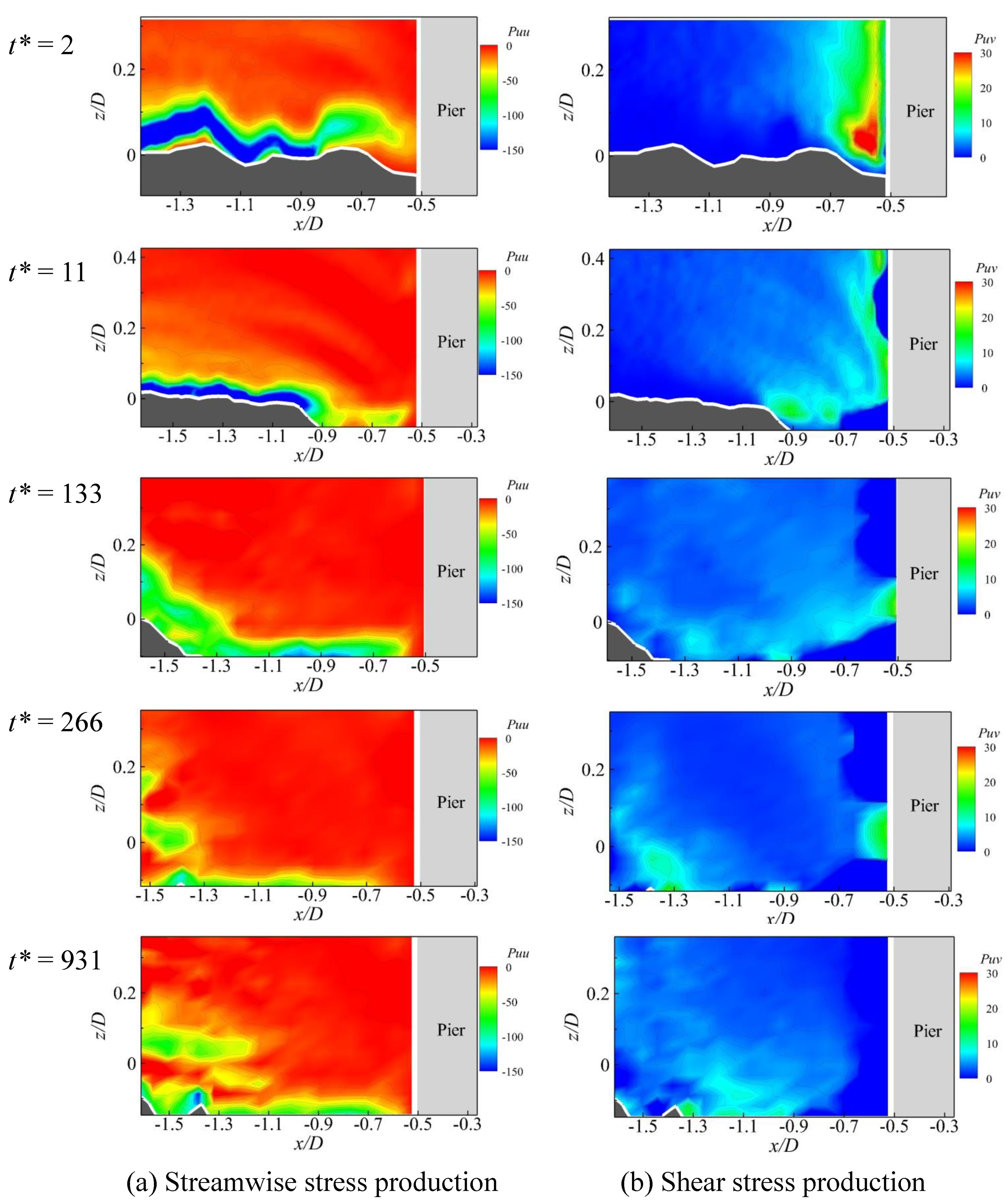
4.4. Production of Turbulent Kinetic Energy

The TKE budget based on the PIV data obtained in present measurement is analyzed. The production terms included in the TKE budget equation are hereby mainly concerned, including the productions from the streamwise stress Puu and shear stress Puv, which are denoted as [42,43]
P u u = u 2 ¯ U x ,   P u v = u v ¯ U z
where u’ and v’ represent streamwise and vertical fluctuating velocity, respectively; U is the time-averaged streamwise velocity.
The contours of TKE production at different time during the pier scouring process are depicted as the following Figure 15. It shows that at the initial scour stage (i.e., t* = 2) the region with high absolute value of Puu is near the bed outside of the scour hole, and the patch of large Puu seems to move towards the front face of the pier. This is similar to the distribution of urms, which illustrates that the turbulence intensity term dominates the TKE production in front of the pier due to streamwise fluctuation. With the development of scour, the region with large Puu moves towards the inside of the scour hole meanwhile the absolute value of Puu is generally decreased because most of turbulent kinetic energy is transported to the scour hole.
Figure 15b clearly shows that the core of the high Puv is located at just the front of the pier at the initial scour stage (t* = 2). In this region, the streamlines experiences large curvature and thus there exists a large shear rate in the streamwise velocity component. The location of its maximum corresponds approximately to the peak position of RSS and TKE. When t* = 11, the maximum Puv is formed at the upstream edge of the scour hole (turning point) as a result of flow separation, which is consistent to the distribution of RSS. This patch of shear production is probably a main contributor to the turbulent kinetic energy. With the development of scour, the region with large Puv moves towards the inside of the scour hole, giving rise to the value of Puv decreased at this region.
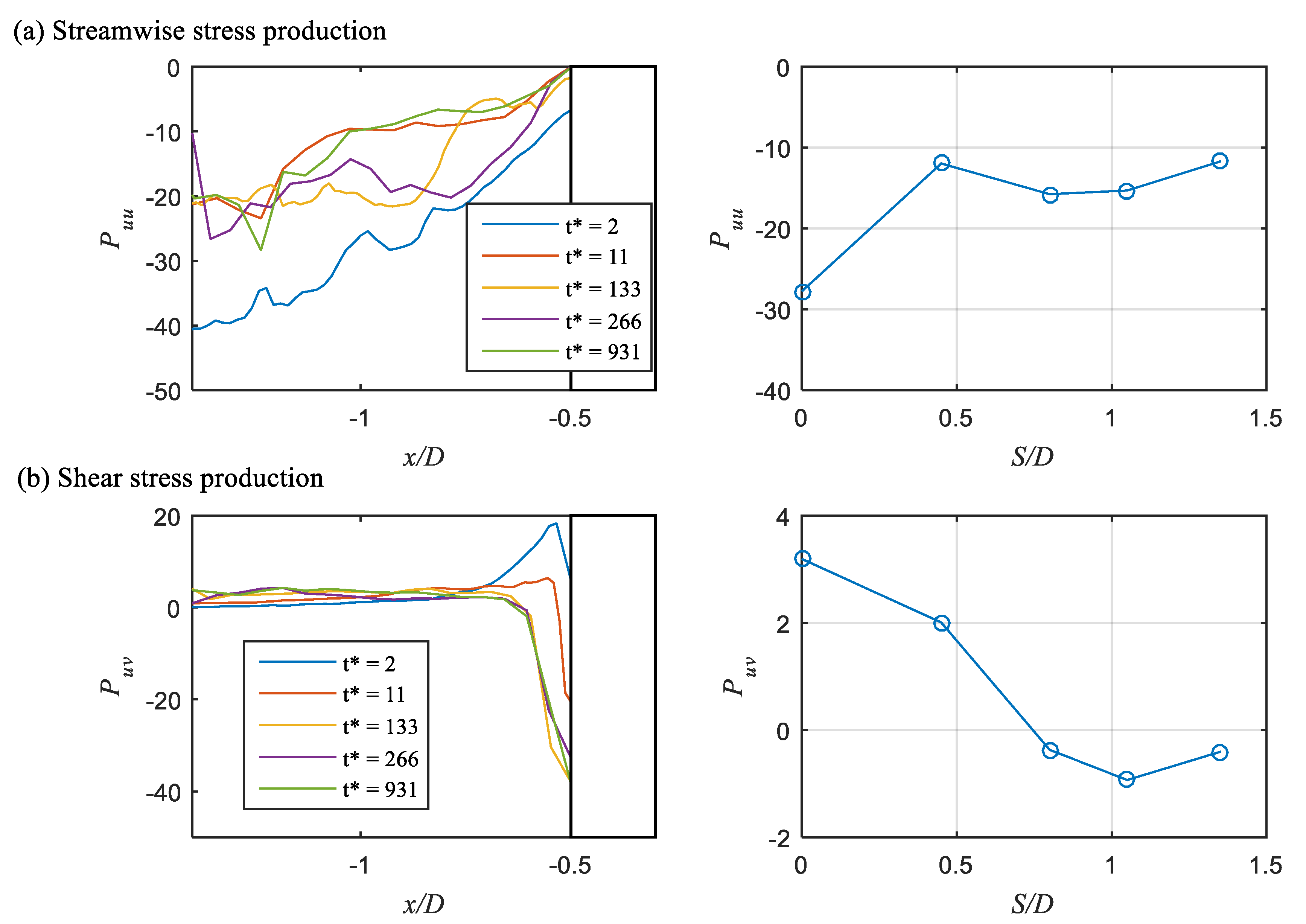
Figure 16 shows the variation of double-averaged TKE budget under different scour depth, in which the left subplot is the velocity variation along the center line for which the value was obtained by averaging the velocities over vertical direction. The corresponding space-averaged results (i.e., by averaging the data in the measured area) versus scour depth were presented in the right subplot. Figure 16a demonstrates that the absolute value of Puu is decreased closing to the pier and almost zero near the front face of the pier. This variation tendency is reasonably similar to the distribution of urms. The absolute space-averaged value for Puu is decreased with increasing scour depth. Figure 16b shows that the Puv is small along the x direction except for the region close to the pier with a significant change to a large absolute value. With the development of scour depth, the space-averaged value of Puv is reduced because most of turbulent kinetic energy is transported into the scour hole.

5. Summary and Conclusions

This paper experimentally investigated the influence of scour development on turbulent flow field in front of a bridge pier. The scour development, including the scour hole evolution and the temporal variation of scour depth around the pier were thoroughly discussed. The flow fields in front of the pier at different instants during the scour process were obtained by the high-resolution PIV measurement. Furthermore, the hydrodynamic characteristics, in terms of the time-averaged velocities, turbulence intensities, Reynolds shear stress, turbulent kinetic energy, and production of turbulent kinetic energy were analyzed in detail.
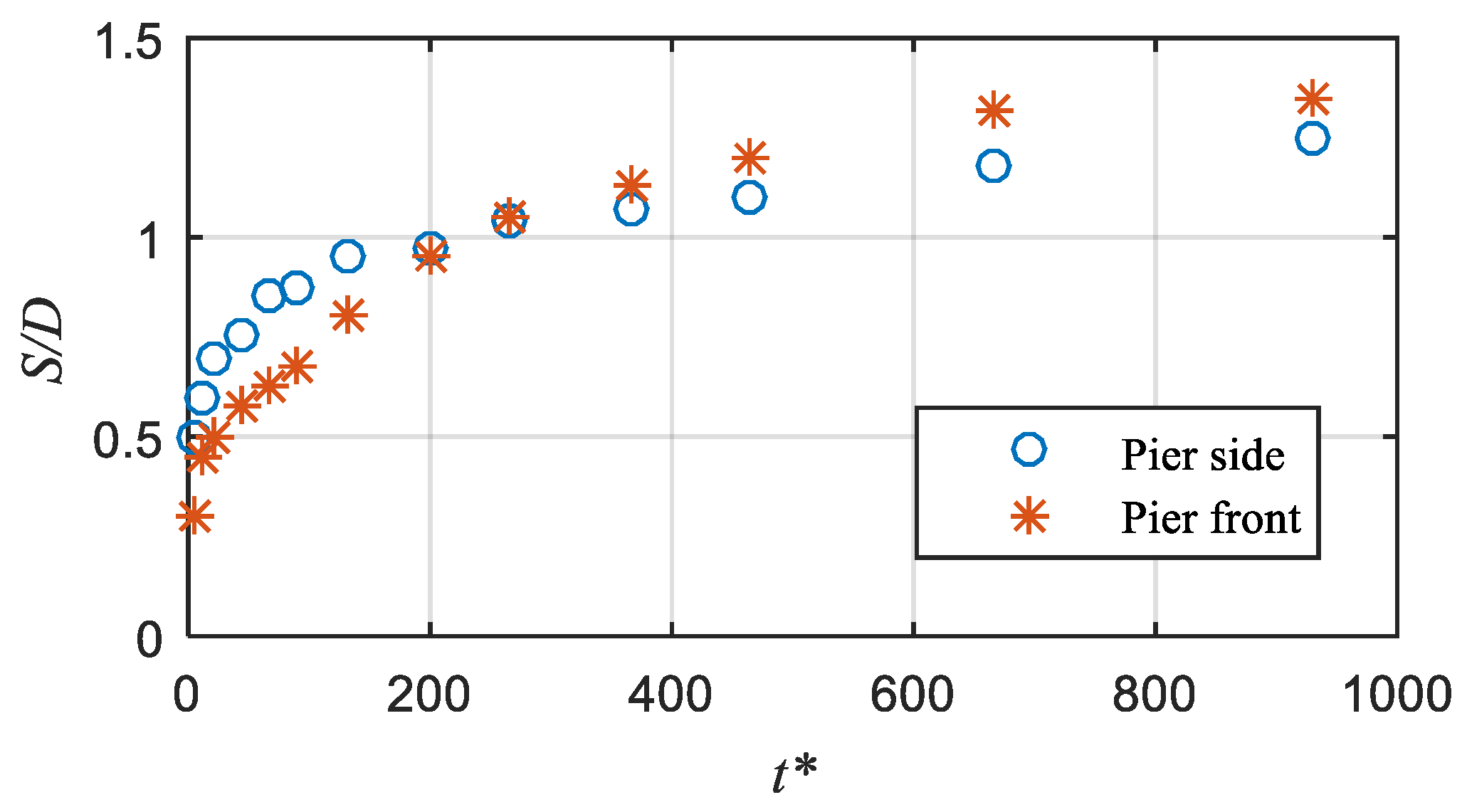
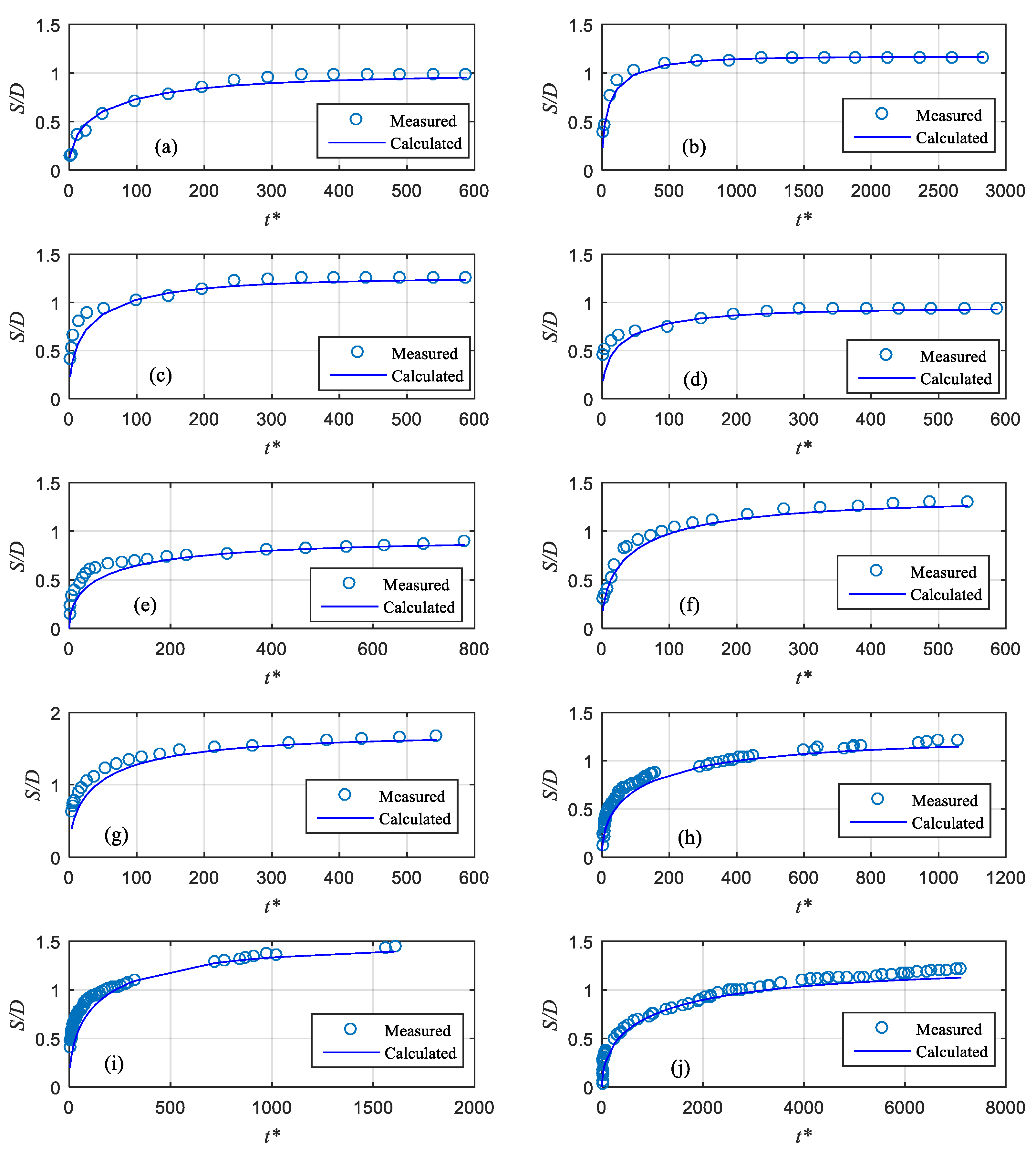
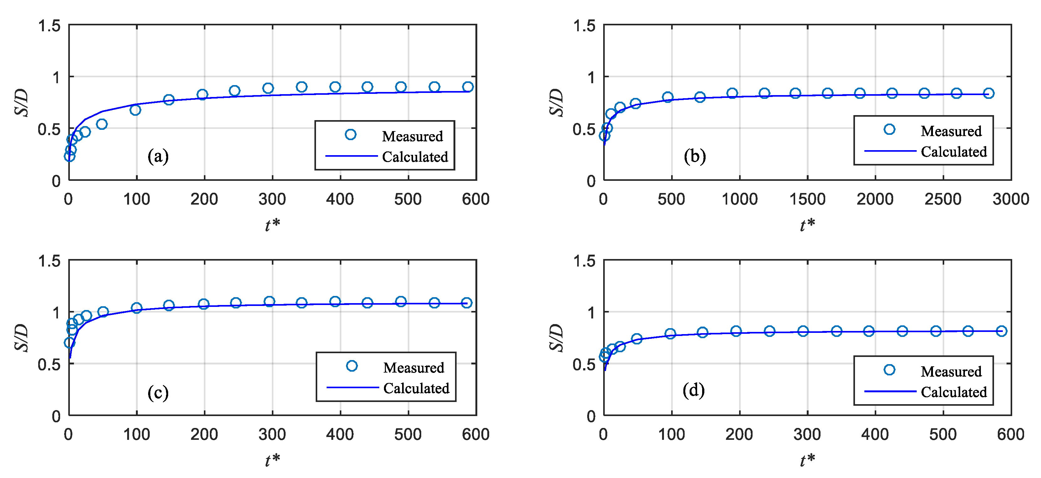
During the scour process, the bed slope upstream of the scour hole at different moment remains almost constant, which is approximately equal to the angle of repose. The scour depth at the pier front exceeds that of the pier side at the later scouring stage. The temporal development of scour depth can be well predicted by a simple practical engineering model based on an exponential function with a change in the two adjustable coefficients (c1 and c2), of which c1 represents the scour rate and c2 is found analytically to be related to the scour hole geometry with a value smaller than 1. Comparison with other previously experimental data demonstrates that the present simple model does a good job of predicting the scour depth observed at both pier front and side.
The flow field indicates that with the scour hole development, the downward flow in front of the pier becomes more prominent, and the flow becomes more turbulent due to the effect of turbulent horseshoe vortex within the scour hole. The variation tendency for both velocities and turbulence intensities along streamwise direction in front the pier shows similarity. The Reynolds shear stress increases with developing scour hole, and the region with large value enlarges and moves upstream of the scour hole. The variation of turbulent kinetic energy with scour depth is relatively complicated rather than monotonic increasing or decreasing. The analysis of TKE budget illustrates that the turbulence intensity term dominates the TKE production in front of the pier due to streamwise fluctuation. With the development of scour, most of TKE production is transported into the scour hole.

Author Contributions

J.L. conducted the experiments, analyzed the data, and wrote the paper; Y.Y. reviewed and edited the paper and provided suggestions for the improvement of the paper; Z.Y. reviewed and provided suggestions during the revision of the paper. All authors have read and agreed to the published version of the manuscript.

Funding

This research was funded by the Basic Funding of the Central Public Research Institutes (TKS190101, TKS20200101) and the Key science and technology projects of Ministry of Transport of China (2019-ZD10-059).

Acknowledgments

The authors would like to thank the editors and the two anonymous reviewers for their constructive comments and suggestions during the revision of the manuscript. The first author expresses sincere gratitude to Meilan Qi for providing the experimental equipment, and also Qigang Chen for the assistance on PIV measurement.

Conflicts of Interest

The authors declare no conflict of interest.

Appendix A

Appendix A.1. Validation of PIV Measurement

The velocity fields measured at the initial flatbed condition were used to compute the turbulence statistics at different streamwise positions. Figure A1 presents the profiles of mean velocity and statistical quantities (turbulence intensity and Reynolds shear stress) at x/D = −3.0 upstream of the pier. The direct numerical simulation (DNS) result by Del Alamo et al. (2004) [44] for a turbulent channel flow at comparable Reynolds number was plotted for comparison. It shows that the experimental profiles agree well with the DNS results except in the upper part of the flow due to the influences of free surface, verifying the present measured results by PIV is reasonable and accurate, and also the turbulent open channel flow is quasi-two-dimensional and fully developed upstream of the cylinder.
Figure A1. Comparison of velocity and turbulence quantities by the present particle image velocimetry (PIV) measurement with direct numerical simulation (DNS) results.
Water 12 02370 g0a1

References

  1. Ettema, R.; Constantinescu, G.; Melville, B.W. Flow-field complexity and design estimation of pier-scour depth: Sixty years since Laursen and Toch. J. Hydraul. Eng. 2017, 143. [Google Scholar] [CrossRef]
  2. Deng, L.; Cai, C.S. Bridge scour: Prediction, modeling, monitoring, and countermeasures-Review. Pract. Period. Struct. Des. Constr. 2010, 15, 125–134. [Google Scholar] [CrossRef] [Green Version]
  3. Sheppard, D.M.; Melville, B.W.; Demir, H. Evaluation of existing equations for local scour at bridge piers. J. Hydraul. Eng. 2013, 140, 14–23. [Google Scholar] [CrossRef]
  4. Qi, M.L.; Li, J.Z.; Chen, Q.G. Comparison of existing equations for local scour at bridge piers: Parameter influence and validation. Nat. Hazards 2016, 82, 2089–2105. [Google Scholar] [CrossRef]
  5. Qi, M.L.; Li, J.Z.; Chen, Q.G. Applicability analysis of pier-scour equations in the field: Error analysis by rationalizing measurement data. J. Hydraul. Eng. 2018, 144. [Google Scholar] [CrossRef]
  6. Pandey, M.; Sharma, P.K.; Ahmad, Z.; Singh, U.K. Evaluation of existing equations for temporal scour depth around circular bridge piers. Environ. Fluid Mech. 2017, 17, 981–995. [Google Scholar] [CrossRef]
  7. Sumer, B.M.; Fredsøe, J. The Mechanics of Scour in the Marine Environment; World Scientific: Singapore, 2002. [Google Scholar]
  8. Cheng, N.S.; Chiew, Y.M.; Chen, X.W. Scaling analysis of pier-scouring processes. J. Eng. Mech. 2016, 142. [Google Scholar] [CrossRef]
  9. Simarro-Grande, G.; Martín-Vide, J.P. Exponential expression for time evolution in local scour. J. Hydraul. Res. 2004, 42, 663–665. [Google Scholar] [CrossRef]
  10. Ben, M.M.; Mossa, M. New approach to predicting local scour downstream of grade-control structure. J. Hydraul. Eng. 2020, 146, 2. [Google Scholar] [CrossRef]
  11. Ben, M.M.; Mossa, M. Scour holes downstream of bed sills in low-gradient channels. J. Hydraul. Res. 2006, 44, 497–509. [Google Scholar] [CrossRef]
  12. Dey, S.; Raikar, R.V. Characteristics of horseshoe vortex in developing scour holes at piers. J. Hydraul. Eng. 2007, 133, 399–413. [Google Scholar] [CrossRef]
  13. Kumar, A.; Kothyari, U.C. Three-dimensional flow characteristics within the scour hole around circular uniform and compound piers. J. Hydraul. Eng. 2012, 138, 420–429. [Google Scholar] [CrossRef]
  14. Kumar, A.; Kothyari, U.C.; Raju, K.G.R. Flow structure and scour around circular compound bridge piers—A review. J. Hydro-Environ. Res. 2012, 6, 251–265. [Google Scholar] [CrossRef]
  15. Yang, Y.L.; Qi, M.L.; Li, J.Z.; Ma, X.D. Evolution of Hydrodynamic Characteristics with Scour Hole Developing around a Pile Group. Water 2018, 10, 1632. [Google Scholar] [CrossRef] [Green Version]
  16. Kirkil, G.; Constantinescu, S.G.; Ettema, R. Coherent structures in the flow field around a circular cylinder with scour hole. J. Hydraul. Eng. 2008, 134, 82–84. [Google Scholar] [CrossRef]
  17. Link, O.; González, C.; Maldonado, M.; Escauriaza, C. Coherent structure dynamics and sediment particle motion around a cylindrical pier in developing scour holes. Acta Geophys. 2012, 60, 1689–1719. [Google Scholar] [CrossRef]
  18. Ben, M.M.; Serio, F.D.; Padova, D.D.; Mossa, M. Hydrodynamic structure with scour hole downstream of bed sills. Water 2020, 12, 186. [Google Scholar]
  19. Lin, C.; Chiu, P.H.; Shieh, S.J. Characteristics of horseshoe vortex system near a vertical plate-base plate juncture. Exp. Therm. Fluid Sci. 2003, 27, 25–46. [Google Scholar] [CrossRef]
  20. Huang, R.F.; Hsu, C.M.; Lin, W.C. Flow characteristics around juncture of a circular cylinder mounted normal to a flat plate. Exp. Therm. Fluid Sci. 2014, 55, 187–199. [Google Scholar] [CrossRef]
  21. Huang, R.F.; Hsu, C.M.; Cheng, T.H. Effects of upstream tetrahedron length on flow characteristics around juncture of circular cylinder and flat plate. Exp. Therm. Fluid Sci. 2018, 92, 295–305. [Google Scholar] [CrossRef]
  22. Schanderl, W.; Jenssen, U.; Strobl, C.; Manhart, M. The structure and budget of turbulent kinetic energy in front of a wall-mounted cylinder. J. Fluid Mech. 2017, 827, 285–321. [Google Scholar] [CrossRef]
  23. Ozturk, N.A.; Akkoca, A.; Sahin, B. Flow details of a circular cylinder mounted on a flat plate. J. Hydraul. Res. 2008, 46, 344–355. [Google Scholar] [CrossRef]
  24. Li, J.Z.; Qi, M.L.; Fuhrman, D.R.; Chen, Q.G. Influence of turbulent horseshoe vortex and associated bed shear stress on sediment transport in front of a cylinder. Exp. Therm. Fluid Sci. 2018, 97, 444–457. [Google Scholar] [CrossRef]
  25. Chen, Q.G.; Yang, Z.L.; Wu, H.J. Evolution of turbulent horseshoe vortex system in front of a vertical circular cylinder in open channel. Water 2019, 11, 2079. [Google Scholar] [CrossRef] [Green Version]
  26. Unger, J.; Hager, W.H. Down-flow and horseshoe vortex characteristics of sediment embedded bridge piers. Exp. Fluids 2007, 42, 1–19. [Google Scholar] [CrossRef] [Green Version]
  27. Beheshti, A.A.; Ataie-Ashtiani, B. Scour hole influence on turbulent flow field around complex bridge piers. Flow Turbul. Combust. 2016, 97, 1–24. [Google Scholar] [CrossRef]
  28. Apsilidis, N.; Diplas, P.; Dancey, C.L.; Bouratsis, P. Effects of wall roughness on turbulent junction flow characteristics. Exp. Fluids 2016, 57, 1–16. [Google Scholar] [CrossRef]
  29. Apsilidis, N.; Diplas, P.; Dancey, C.L.; Bouratsis, P. Time-resolved flow dynamics and Reynolds number effects at a wall-cylinder junction. J. Fluid Mech. 2015, 776, 475–511. [Google Scholar] [CrossRef]
  30. Soulsby, R.L.; Whitehouse, R.J.S. Threshold of sediment motion in coastal environments. In Pacific Coasts and Ports’ 97: Proceedings of the 13th Australasian Coastal and Ocean Engineering Conference and the 6th Australasian Port and Harbour Conference; Centre for Advanced Engineering (CEA): Christchurch, New Zealand, 1997; Volume 1. [Google Scholar]
  31. Scarano, F. Iterative image deformation methods in PIV. Meas. Sci. Technol. 2002, 13, R1–R19. [Google Scholar] [CrossRef]
  32. Chen, Q.G.; Adrian, R.J.; Zhong, Q.; Li, D.X.; Wang, X.K. Experimental study on the role of spanwise vorticity and vortex filaments in the outer region of open-channel flow. J. Hydraul. Res. 2014, 52, 476–489. [Google Scholar] [CrossRef]
  33. Chen, Q.G.; Qi, M.L.; Zhong, Q.; Wang, X.K. Experimental study on the multimodal dynamics of the turbulent horseshoe vortex system around a circular cylinder. Phys. Fluids 2017, 29, 015106. [Google Scholar] [CrossRef]
  34. Qi, M.L.; Li, J.Z.; Chen, Q.G.; Zhang, Q.F. Roughness effects on near-wall turbulence modelling for open-channel flows. J. Hydraul. Res. 2018, 56, 648–661. [Google Scholar] [CrossRef]
  35. Simarro, G.; Fael, C.M.S.; Cardoso, A.H. Estimating equilibrium scour depth at cylindrical piers in experimental studies. J. Hydraul. Eng. 2011, 137, 1089–1093. [Google Scholar] [CrossRef]
  36. Bouratsis, P.; Diplas, P.; Dancey, C.L.; Apsilidis, N. Quantitative spatio-temporal characterization of scour at the base of a cylinder. Water 2017, 9, 227. [Google Scholar] [CrossRef]
  37. Yang, Y.L.; Qi, M.L.; Li, J.Z.; Wang, X. Experimental study of scour around pile groups in steady flows. Ocean Eng. 2020, 195, 106651. [Google Scholar] [CrossRef]
  38. Larsen, B.E.; Fuhrman, D.R.; Baykal, C.; Sumer, B.M. Tsunami-induced scour around monopile foundations. Coast. Eng. 2017, 129, 36–49. [Google Scholar] [CrossRef] [Green Version]
  39. Alabi, P.D. Time Development of Local Scour at Bridge Pier Fitted with a Collar. Ph.D. Thesis, University of Saskatchewan, Saskatoon, SK, Canada, 2006. [Google Scholar]
  40. Yanmaz, A.M. Temporal variation of clear water scour at cylindrical bridge piers. Can. J. Civ. Eng. 2006, 33, 1098–1102. [Google Scholar] [CrossRef]
  41. Justesen, P. A note on turbulence calculations in the wave boundary layer. J. Hydraul. Res. 1991, 29, 699–711. [Google Scholar] [CrossRef]
  42. Ghodke, C.D.; Apte, S.V. DNS study of particle-bed-turbulence interactions in an oscillatory wall-bounded flow. J. Fluid Mech. 2016, 792, 232–251. [Google Scholar] [CrossRef]
  43. Ghodke, C.D.; Apte, S.V. Spatio-temporal analysis of hydrodynamic forces on the particle bed in an oscillatory flow environment. J. Fluid Mech. 2018, 841, 167–202. [Google Scholar] [CrossRef]
  44. Del Alamo, J.C.; Jimenez, J.; Zandonade, P.; Moser, R.D. Scaling of the energy spectra of turbulent channels. J. Fluid Mech. 2004, 135, 135–144. [Google Scholar] [CrossRef] [Green Version]
Figure 1. Experimental setup: (a) global side view; (b) local top view.
Water 12 02370 g001
Figure 2. Photographs of local scour hole around the pier at the time of (a) t* = 11; (b) t* = 133; (c) t* = 266; and (d) t* = 931.
Water 12 02370 g002
Figure 3. Scour morphology around the pier at the time of (a) t* = 11; (b) t* = 133; (c) t* = 266; and (d) t* = 931.
Water 12 02370 g003
Figure 4. Scour profile along the centerline in front of the pier at different time.
Water 12 02370 g004
Figure 5. Measured scour depths versus time at the front and side faces of the pier.
Water 12 02370 g005
Figure 6. Comparison between the predicted and measured temporal development of scour depth at the (a) side and (b) front face of the pier.
Water 12 02370 g006
Figure 7. Comparison of temporal scour depth at pier front calculated by the present exponential equation with other previously experimental data: (ad) Pandey et al. (2018) [6]; (eg) Yanmaz (2006) [40]; (hj) Alabi (2006) [39].
Water 12 02370 g007
Figure 8. Comparison of temporal scour depth at pier side calculated by the present exponential equation with the experimental data from Pandey et al. (2018) [6]. (a) Test 1; (b) Test 2; (c) Test 3; (d) Test 4.
Water 12 02370 g008
Figure 9. Contours and vectors of time-averaged velocity at different time in the pier scouring process.
Water 12 02370 g009
Figure 10. Velocity distributions along the center line at different time in the pier scouring process and the corresponding space-averaged value versus dimensionless pier scour depth. (a) streamwise velocity, (b) vertical velocity.
Water 12 02370 g010
Figure 11. Contours of turbulence intensities at different time in the pier scouring process. (a) streamwise turbulence intensity, (b) vertical turbulence intensity.
Water 12 02370 g011
Figure 12. Turbulence intensities distributions along the center line at different time in the pier scouring process and the corresponding space-averaged value versus dimensionless pier scour depth.
Water 12 02370 g012
Figure 13. Contours of Reynolds shear stress and turbulent kinetic energy at different time in the pier scouring process.
Water 12 02370 g013
Figure 14. Reynolds shear stress and turbulent kinetic energy along the center line at different time in the pier scouring process and the corresponding space-averaged value versus dimensionless pier scour depth. (a) Reynolds shear stress, (b) turbulent kinetic energy.
Water 12 02370 g014
Figure 15. Contours of turbulent kinetic energy production at different time in the pier scouring process. (a) streamwise stress production, (b) shear stress production.
Water 12 02370 g015
Figure 16. Production of turbulent kinetic energy along the center line at different time in the pier scouring process and the corresponding space-averaged value versus dimensionless pier scour depth. (a) streamwise stress production, (b) shear stress production.
Water 12 02370 g016
Table 1. Summary of experimental data and parameters used for current model validation.
Test No.Data SetD (m)U0 (m/s)h (m)d50 (mm)ReDFrDd50/D
1Pandey et al. (2018) [6]0.1350.740.12510.799,0000.6430.079
20.1150.530.18.660,4000.4990.075
30.1350.70.138.693,7000.6090.064
40.1150.70.14.3879,8000.6590.038
5Yanmaz (2006) [40]0.0570.230.071.0713,0000.3080.019
60.0570.260.090.8414,9000.3520.015
70.0570.330.140.8418,8000.4440.015
8Alabi (2006) [39]0.1150.250.230.5328,5000.2350.005
90.0730.250.150.5318,1000.2960.007
100.1150.200.230.5322,8000.1880.005
Note: D is pier diameter; U0 is approach flow velocity; h is flow depth; d50 is sediment median size; ReD = U0D/ν; FrD = U0/(gD)0.5.

