Abstract
Distributed and semi-distributed hydrological modeling approaches commonly involve the discretization of a catchment into several modeling elements. Although some modeling studies were conducted using triangulated irregular networks (TINs) previously, little attention has been given to assess the impact of TINs as compared to the standard catchment discretization techniques. Here, we examine how different catchment discretization approaches and radiation forcings influence hydrological simulation results. Three catchment discretization methods, i.e., elevation zones (Hypsograph) (HYP), regular square grid (SqGrid), and TIN, were evaluated in a highly steep and glacierized Marsyangdi-2 river catchment, central Himalaya, Nepal. To evaluate the impact of radiation on model response, shortwave radiation was converted using two approaches: one with the measured solar radiation assuming a horizontal surface and another with a translation to slopes. The results indicate that the catchment discretization has a great impact on simulation results. Evaluation of the simulated streamflow value using Nash–Sutcliffe efficiency (NSE) and log-transformed Nash–Sutcliffe efficiency (LnNSE) shows that highest model performance was obtained when using TIN followed by HYP (during the high flow condition) and SqGrid (during the low flow condition). Similar order of precedence in relative model performance was obtained both during the calibration and validation periods. Snow simulated from the TIN-based discretized models was validated with Moderate Resolution Imaging Spectroradiometer (MODIS) snow products. Critical Success Indexes (CSI) between TIN-based discretized model snow simulation and MODIS snow were found satisfactory. Bias in catchment average snow cover area from the models with and without using imputed radiation is less than two percent, but implementation of imputed radiation into the Statkraft Hydrological Forecasting Toolbox (Shyft) gives better CSI with MODIS snow.
1. Introduction
Accurate runoff prediction is one of the fundamental challenges for effective and sustainable water resource management in the Himalaya region. Reliable meteorological forcing data and accurate land cover information at a range of spatial and temporal scales are critical to effective runoff prediction, and for water resource management [1]. The main challenge to estimate (or measure) meteorological forcing variables comes from the fact that they vary both in space and time as a function of meteorological inputs. Spatial variability of topography and land use cover types also adds to the complexity of the problem [2].
In the past, several hydrological models have been developed for use in various applications. Some of these models include SRM [3], HEC-HMS [4], J2000 [5], Statkraft’s Hydrological Forecasting Toolbox (Shyft) [6], etc. Unlike other hydrological models, Shyft provides an optimized platform for the implementation of many well-known hydrological models from conceptual to physically based distributed hydrological models. Most of the distributed hydrological models discretize the catchment and derive terrain attributes from digital elevation models (DEMs). Most commonly used catchment discretization methods in hydrological applications are grid-based [7,8,9,10], and elevation band (hypsography) based [11,12,13]. Recently, triangulated irregular network (TIN)-based discretized hydrological models are also used for discharge simulations [14,15], but to date TIN-based distributed hydrological models are not tested in the Himalaya catchments. Although the use of grid and elevation based discretized models are more prevalent due to their simplicity and ease of implementation [16,17], TIN-based discretized models have a better potential of accurately representing topographic features than grids and hypsography [14]. In this context, Shyft can be a valuable tool to evaluate different models as it have the ability to take the terrain heterogeneity into account and provide distributed output variables. Shyft can be used to test different functioning hypotheses from which simplified and/or predictive models can be derived for more operational purposes. If reliable output variables are expected, Shyft parameters can be estimated a priori from available information. Verification of these models behavior can be performed not only on the discharge at the outlet but also at intermediate variables (such as snow cover area, snow water equivalent, etc.) leading to a multiobjective verification. The main drawback of the current version of the Shyft is that it uses conceptual models.
The topographical information such as snow cover area is one of the most important variables for the application of hydrological model [18,19,20], and can dominate local and regional climate, and hydrology. Snow and glacier strongly influence the regional radiation budget with its high albedo and acts as an insulation, controlling snow accumulation and melt [21]. In this regard, accurate representation of snow cover at micro-scale of spatial variation is required to provide accurate and timely information on water availability and its management. Many distributed hydrological models are commonly employed to quantify snow cover area and snow water equivalent (SWE). All models have strengths and limitations [22,23]. For example, current model-based snow simulation approaches in Shyft are limited to the radiation received on a horizontal plane surface, which introduce a certain degree of uncertainty in the radiation received by the surface. In view of this, we have implemented the imputed radiation algorithm following a similar approach as in Allen et al. [24] in order to account for the effect of slope and aspect on incident radiation.
Remote sensing is an alternative powerful tool that offers the ability to examine quantitatively the physical properties of snow [25]. A well-known example is a MODerate Resolution Imaging Spectroradiometer (MODIS) instrument which can provide daily snow cover fraction with nearly global coverage at the resolution of 500 km [26,27]. For regional snow cover mapping, the MODIS satellite sensors are particularly appealing due to their high spatiotemporal resolution [28]. In this regard, validation of snow cover area simulated from the Shyft with MODIS will also add the most important aspect to hydrological simulation.
Despite a number of previous modeling studies, the conversion of a highly variable meteorological field into a spatially-distributed snow response remains an unanswered, open question. This is primarily due to the fact that meteorological processes operating in a watershed are highly heterogeneous and interconnected in the system [29]. Although some modeling studies were conducted using TIN previously, little attention has been given to assess the impact of TIN as compared to the standard catchment discretization technique over the Himalayan catchment. In this regard, we have implemented imputed radiation following a similar approach to Allen et al. [24] on different catchment discretized models (i.e., elevation band, regular spaced grid, and TIN) for calculating snow cover area using PT_GS_K stack of Shyft (https://shyft.readthedocs.io). The primary method for the simulation and distribution of snow cover area in PT_GS_K is in the matrix format of equally spaced elevation points. A data point in a matrix does not allow meaningful analysis of the terrain. Hence we hypothesize that the Shyft using the TIN for discretizing a watershed should enable a better prediction of the change in a runoff pattern caused by a change in a watershed characteristics. Finally, we tried to answer the question, what value does the TIN format offer over a matrix format for this particular application. This study also presents and evaluates the different catchment discretization models and the newly added translated radiation algorithm on the snow cover area and discharge simulations. As of our best knowledge, TIN-based discretized model with imputed radiation has not been applied before to simulate discharge in the Himalayan river catchments.
This manuscript is novel providing a capability to simulate discharge over the Himalayan catchment using community modeling framework. This paper will help in an understanding of downscale and translated radiation measurements onto the inclined surface and its impacts on hydrological response. An understanding of the relationships between catchment discretization and hydrological response and a cross-validation of hydrological model snow simulation using MODIS derived snow cover data will help to fill existing knowledge gap over the region. Hydrological model calibration and validation was carried out between 2000 to 2009. Selection of calibration and validation years was based on the observations data quality (less missing data), particularly observed discharge. In the paper, the materials and method, study area, hydrological models, model forcing datasets, and validation datasets are presented in Section 2. Results are presented in Section 3, while the discussion is presented in Section 4. Finally, conclusions are presented in Section 5.
2. Materials and Methods
2.1. Hydrologic Model Framework
The Statkraft Hydrological Forecasting Toolbox (Shyft, https://gitlab.com/shyft-os) was used in this study. Shyft provides an optimized platform for the implementation of well known hydrological models [6]. The high-performance generic time series framework in Shyft allows for rapid calculations of hydrologic response at the regional to a cell scale. The standard models in Shyft, i.e., PT_GS_K, PT_SS_K, and PT_HS_K, mainly differ in their snow mass balance methods calculations. The main model forcing variables are atmospheric temperature, precipitation, wind speed, relative humidity, and shortwave radiation, given in Table 1. Shyft works down from the regional level to the cell level by distributing the input variables and parameters to the georeferenced grid cell (described in catchment discretization technique). In the model, Bayesian kriging approach is used to distribute point temperature data over the catchment, while the inverse distance weighting approach is used for other forcing variables. The PT_GS_K model is the widely used as compared to the remaining models of Shyft (Teweldebrhan, 2019). Potential evapotranspiration in this model is calculated by Priestley-Taylor method [30]. Actual evapotranspiration is assumed to take place from snow-free area and is estimated as a function of potential evapotranspiration, and a scaling factor. Gamma snow routine (Section 2.1.1) is used for snowmelt, sub-grid snow distribution, and mass balance calculation. A simple storage–discharge function is used for catchment response calculation [31,32]. The catchment response function is based on the storage-discharge relationship concept described in Kirchner [32] and represents the sensitivity of discharge to storage changes given by Equation (1). As discharge is generally nonlinear and varies by many orders of magnitude, the recommended approach is to use log-transformed discharge values to avoid numerical instability.
where P, Q, and E are the rate of precipitation (from snow-melt and rain), discharge, and actual evapotranspiration (from snow-free area) in units of depth per time. The concept behind this method is that the catchment sensitivity of discharge to changes in storage i.e., , can be estimated from the time series of the discharge alone through fitting empirical functions to the data such as the quadratic equation, and is given by Equation (2) [32].
where , , and are the catchment specific outlet parameters (hereafter called Kirchner parameters) obtained during the model calibration. There is no routing into the model, but Kirchner parameters response delays outflow from precipitation and snow/glacier melt.

Table 1.
Summary of hydrological model input data.
2.1.1. Snow and Glacier Balance
The Gamma snow routine uses an energy balance approach (Equation (3)) for snow ablation, and the snow depletion curve represented by gamma distribution for snow distribution. The energy balance approach in the Gamma snow routine follows similar approach as used in DeWalle and Rango [33]. The net energy flux at the surface available for snow ablation is expressed as
where S is the net shortwave radiation; and are the incoming and outgoing longwave radiation; respectively, and represent sensible and latent heat fluxes, respectively; and is the net ground heat energy flux and is calculated using bulk-transfer approach. Two parameters defining wind profile—intercept (wind constant) and slope (wind scale)—are determined through either calibration or prescribed (Table 2). For a given time step (t), the snow albedo at each grid cell depends on the minimum and maximum albedo values as well as the albedo decay rate, temperature, and snowmelt e.g., Hegdahl et al. [9]:
Table 2.
Model calibration parameters with upper and lower limits. Prescribed parameters are marked with *. Parameters only used in radiation model are marked with **.
In Equation (4), FDR and SDR denote fast and slow snow cover decay rates, respectively. In this study, and are estimated during the model calibration.
Within the gamma snow routine, precipitation falling in each grid cell is classified as solid or liquid depending on a threshold temperature (tx), and the actual grid cell temperature. Snow distribution to each cell is estimated by using a three-parameter gamma probability distribution [7]. Snowmelt depth is calculated by multiplying (available energy) with the latent heat of fusion for water.
The temperature index model [34] is used in the model for glacier melt calculation. The glacier reservoir is assumed to be infinite and glacier area is assumed to be constant throughout the study periods. In a grid cell, snow is assumed to melt first from glacier cover/free areas, and glacier melt only happens from glacial areas that are snow-free. Obtained runoff depth per grid cell is summed with snowmelt depth from the gamma snow routine and converted to volume by multiplying the area of each grid cell before Kirchner routine.
2.1.2. Study Catchment and Data
The study has been conducted in the Marsyangdi-2 River catchment (Figure 1), Nepal. It is located between 2810′21″ N to 2854′11″ N and 8347′24″ E to 8448′04″ E. The catchment has a total area of 3001 sq. km, of which 80% lies above the elevation of 3000 m asl. The catchment elevation ranges from 641 m asl to 7924 m asl with a mean elevation of 4377 m asl, and mean slope of 29.34. Marsyangdi-2 river is a tributary of the Narayani river catchment (Figure 1). It originates from the southern edge of the Tibetan Plateau, flows through Nepal to India, and drains into the Ganges River. Approximately 24% of area is covered by glaciers [35]. The hydrological regime is heavily influenced by seasonal weather variations. The seasons are defined as monsoon (June to September), post-monsoon (October to November), winter (December to February), and pre-monsoon (March to May) [36]. Approximately 80% of the total annual precipitation occurs during the monsoon period [37,38].
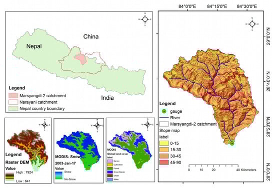
Figure 1.
Location map of the Marsyangdi-2 River catchment.
The Narayani River catchment lies also in the primary hydropower development region of Nepal, providing 44% of the total national electric supply [39]. Some of the operating hydropower development projects in this catchment include Marsyangdi (69 MW) and middle marsyangdi (70 MW). The upper marsyangdi (600 MW), lower Manang marsyangdi (100 MW), and Nyadi (30 MW) are some of the hydropower project currently under different stages of development. Therefore, the study area is an important catchment in Nepal from hydropower perspective.
2.1.3. Meteorological Forcing and Observed River Gauge Data
Standard model forcing data are temperature, precipitation, relative humidity, wind speed, and incoming short wave radiation. All these model forcing were obtained from Water and Global Change (WATCH) Forcing Data ERA-Interim (WFDEI). Selection of the forcing data sets for the hydrological model was based on the prior study by Bhattarai et al. [10]. WFDEI is a global meteorological forcing data set at 0.5× 0.5 horizontal resolution obtained by bias-correcting ERA-I data [40,41]. It covers the period 1979–2016 and contains eight meteorological variables at a 3 h time step [42]. WFDEI then corrects ERA-Interim for precipitation biases using data from the Climatic Research Unit (CRU) or the Global Precipitation Climatology Center (GPCC). In this study, GPCC products were preferred to CRU because of their higher resolution and data quality [40,41]. The WFDEI data set is freely available online from ftp.iiasa.ac.at.
Daily observed river discharge data (observation periods: 2000–2010) at Marsyangdi_2 River 28.2036 N, 84.403 E) are obtained from the Department of Hydrology and Meteorology (DHM), Government of Nepal (GoN). The catchment is highly influenced by seasons as more than 70% of total annual discharge flows from June to September. Highest daily mean discharge is observed during August (386.7 m/s) and low mean discharge is observed in February (30.5 m/s), and daily mean observed discharge is 133.85 m/s. Thus, the obtained discharge data from the DHM GoN was used for the model validation purpose.
2.1.4. MODIS Snow Product, Topographical, and Land Cover Data Sets
In this study, the standard eight-day MODIS Terra and Aqua snow cover products, MOD10A1 and MYD10A1, are chosen for the analysis. They contain snow cover, snow albedo, fractional snow cover, and quality assessment (QA) data in a compressed HDF-EOS format along with corresponding metadata. Only snow cover information is used in the study. Both Aqua and Terra products are with 463.3 m spatial resolution in sinusoidal projection. Frequent cloud cover is one of the major challenges when using MODIS and other optical remote sensing data in the Himalayan region [43]. MOD10A1 was successfully used in earlier studies [44,45,46]. However, Rittger et al. [47] and Toure et al. [48] showed that the MODIS data can be systematically biased compared to Landsat ETM+ snow cover data in the mountainous regions. The average root mean square error (RMSE) between Landsat ETM+ and MOD10A1 snow cover fraction over the Nepal Himalaya was 0.23 [48]. Thus, a composite data set was formed, following Muhammad et al.’s [49] approach, using data retrieved from the Aqua and Terra products in order to minimize the effect of clouds and other sources.
A land cover map (0.3× 0.3, resolution) providing forest cover, lake cover, glacier cover, and reservoir cover of the study area is extracted from the GlobCover Project [50]. Digital Elevation Model (DEM) of 90 m spatial resolution from the Shuttle Radar Topography Mission (SRTM) [51] is used in the study.
2.2. Catchment Discretization Technique
The study catchment was delineated using an automatic catchment delineation method described by Akram et al. [52]. The delineated catchment was further discretized into modeling elements using three methods.
2.2.1. Triangulated Irregular Network (TIN)
TIN is a vector-based data structure comprising a triangular network of vertices with associated coordinates (x, y, z) connected by edges. TIN utilizes the original sample points to constitute many nonoverlapping triangles that cover the entire region. Spacing and shape of the triangles are determined by the terrain and by the desired degree of fit. The mathematical basis for a TIN construction is the Delaunay triangulation methods described in Field [53] and Hjelle and Dæhlen [54], and is based on a principle of maximizing the minimum angle of all triangles produced by connector lines to nearest neighbor points. The TIN interpolation method is an altitude interpolation algorithm, this makes it possible to distribute hydrometeorological forcing variables more correctly for hydrological simulations [55].
Rasputin (https://github.com/expertanalytics/rasputin) is used for generating TIN terrain models of the study area. It can convert a point set of coordinates to a TIN using Delaunay triangulation methods. Specifically, it has been developed to convert Digital Elevation Models (DEMs) into simplified triangulated surface meshes. Rasputin generates catchment TIN using the provided DEM and also calculates physical parameters of each TIN facet, such as slope, area, and aspect, from the TIN geometry. The Rasputin software requires wkt-file describing the catchment polygon, which is easily obtained from shapefiles generated by Qgis. Rasputin is freely available under GNU GPLv3 license.
In the study, TINs with different numbers of cells were generated with the help of Rasputin and DEM [56]. The generated TINs with different number of cells are used for the model calibration and validation. The Nash–Sutcliffe Efficiency (NSE; see Section 2.4.1) value was used for evaluating the performance of the models with particular numbers of TIN cells. Implementing the spatially distributed parameters for the TIN with different number of cells yielded different simulation performance when compared to the observations over the calibration (2000–2004) and validation (2005–2009) periods. As expected, model efficiency in terms of NSE increased with increasing number of TINs (Figure 2). However, after reaching a certain number of cells no further improvement in NSE was found, indicating the limit for Shyft to utilize terrain data. The number of cells corresponding to this limit was considered as an optimum i.e., 671 cells (with median area of 4 km ) (see Figure 2).
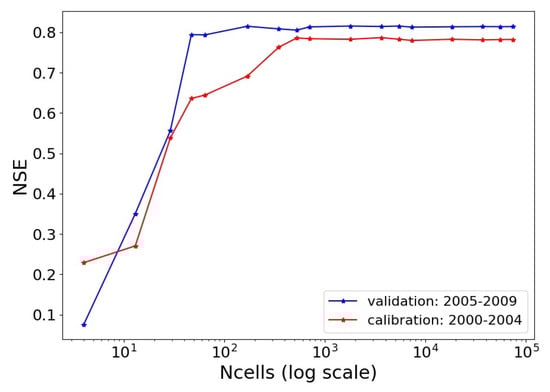
Figure 2.
Scatter plot between Nash–Sutcliffe Efficiency (NSE) and number of Triangulated Irregular Network (TIN) cells (Ncells).
2.2.2. Regular Space Grid
Vector creation tools under Qgis geoalgorithms were used for creating regular space grid cells. Due to the ease of comparison with TIN, a grid mesh with an area of 4 km was selected for this study. Unlike TIN, each grid cell is connected to either four or eight adjacent neighbors, the single resolution inherent in raster grids. The physical parameters (slope, aspect, elevation, latitude, and longitude) of each cell at the centroid (center point) are calculated by using vector geometry tools under Qgis geoalgorithms and further used for distributing the hydrometeorological forcing.
2.2.3. Hypsography (Elevation Zone)
In this study, the catchment area was divided into ten elevation zones. Mean elevation, aspect, and slope of each zone were calculated and further used for the distributing the hydrometeorological forcing. Figure 3 shows discretization of the study catchment using TIN, regular space grid, and elevation bands.
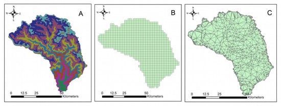
Figure 3.
Catchment discretization by (A) hypsographic, (B) regular space grid, and (C) TIN methods.
2.2.4. Implementation of New Radiation Algorithm in the Shyft
Daily incoming shortwave radiation (from forcing data) falling over the inclined surface with specified slope and aspect was calculated using the methods described by Allen et al. [24]. The procedure assumes each grid/TIN surface has uniform slope. Thus, effects of protruding surrounding terrain were not considered. This simplification facilitates implementation of the procedure within Shyft in energy balance calculation for snow mass balance and in Priestley–Taylor-based potential evapotranspiration calculations.
2.3. Model Construction, Calibration, and Validation
Combination of different catchment discretization methods and radiation algorithms resulted in different models (Table 3). Model forcing datasets was interpolated to each geometric center of cells/TIN using Kriging (for temperature) and IDW methods (for precipitation, wind speed, relative humidity, and incoming shortwave radiation). Details about the interpolation methods are explained in detail in Bhattarai et al. [10]. Each model was calibrated and validated separately. Calibration and prescribed parameters are given in Table 2. Manual calibration can be time-consuming and subjective; therefore, an automatic calibration was carried out using CREST v.2.1, the Shuffle Complex Evolution University of Arizona (SCE-UA) [57]. As described in Bhattarai et al. [10], the calibration procedure involves the selection of samples in the parameter space through the use of competitive evolution schemes, such as the simplex scheme, to reproduce better the observations. After several iterations, either due to convergence or when the maximum number of iteration is reached, the best set of parameter values based on the Nash–Sutcliffe coefficient of efficiency (NSE) is determined. The model was validated with the observed discharge. A cross-validation technique was used, where the optimal model identified in the first periods, i.e., years 2000–2004 was validated during the second period, i.e., 2005–2009, and vice-versa. For convention, different names were given to the model-discretization combinations (Table 3).
Table 3.
Different models with descriptions.
2.4. Evaluation Metrics
2.4.1. Nash–Sutcliffe Efficiency (NSE)
The NSE [58] was used (Equation (5)) to quantitatively evaluate the degree of agreement between observed and simulated discharge. NSE is commonly used to assess the predictive power of hydrological models and its value can range from −∞ to 1. An efficiency of 1 corresponds to a perfect match of simulated to observed discharge values. However, the NSE calculated using raw values tends to overestimate model performance during peak streamflow and to underestimate during low-streamflow conditions [23,59]. To partly overcome this problem, NSE is often calculated with log-transformed observed and modeled values. In this study, both NSE and NSE with log-transformed streamflow values (LnNSE) were thus employed as streamflow efficiency metrics.
where , , and are simulated discharge, observed discharges, and arithmetic mean for observed discharges, respectively.
2.4.2. Critical Success Index (CSI)
We determine the agreement between observed (MODIS) and simulated snow via CSI [60]. It is also known as the Threat Score (TS), combines different aspects of the POD and FAR, describing the overall skill of the simulation relative to reference observation [61]. The value of the CSI score ranges between 0 and 1, with 1 being the ideal score. The formula for CSI is defined as Equation (6), and two-dimensional contingency table fit for evaluating observed and simulated binary events is given in Table 4 [23].
Table 4.
Set-up of the 2 × 2 contingency table for binary snow cover data comparison. O and S, respectively, represent observed and simulated binary snow cover and the subscripts refer to a snow-free (0) and snow-covered (1) grid cell.
Shyft generates fractional snow cover area (fSCA) as one of its main output variables. Thus, in order to convert the fractional snow cover area into binary values, a threshold fSCA value of 0.4 was used to distinguish between snow and snow free cells.
3. Results
3.1. Intercomparison of the Catchment Discretization Methods
The different catchment discretization methods resulted in different number and distribution of computational cells with in the study catchment. The fixed median area of TIN cells (4 km) has yielded to lower number of computational cells (671) as compared to the regular square grid (839). The distribution of cells across the elevation range of the study catchment shows that most of the cells fall within the elevation range of 4000 to 6000 m asl. Most of the reductions in the number of computational cells when using TIN were also obtained in this elevation range (Figure 4). TIN cell areas vary from 0.16 to 15.3 km, while in the hypsographic discretization method, zonal areas range from 6.9 to 726.8 km (Table 5).
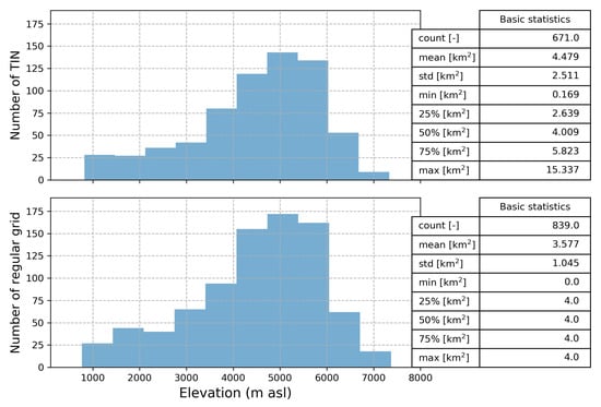
Figure 4.
TIN and grid cell distribution across the elevation ranges in Marsyangadhi_2 catchment.
Table 5.
Hypsographical discretization and zonal characteristics. CID represents catchment number.
Remarkable differences are observed in grid/TIN area distributions with respect to aspect. In regular space square grid, a higher percentage of area is facing towards southwest direction, while in TIN a higher percentage of area is facing towards northeast direction (Figure 5). Differences in area distribution with respect to aspect in different discretization methods ultimately result in differences in snow/glacier cover area in the catchment.
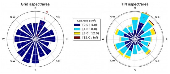
Figure 5.
Cell area distribution with respect to aspect. Numbers in the radius stands for percentage area for respective aspect.
3.2. Evaluation of Catchment Discretization and Imputed Radiation on Streamflow Efficiency
Figure 6 shows the hydrograph of the measured and simulated discharges at Marsyangdi_2 station for calibration and validation periods and different model configurations. The different catchment discretization methods resulted to different model efficiency. Both the calibration and validation results show a good agreement between observed and modeled daily discharge values in terms of NSE (>0.75). However, annual peak values are underestimated by all models.
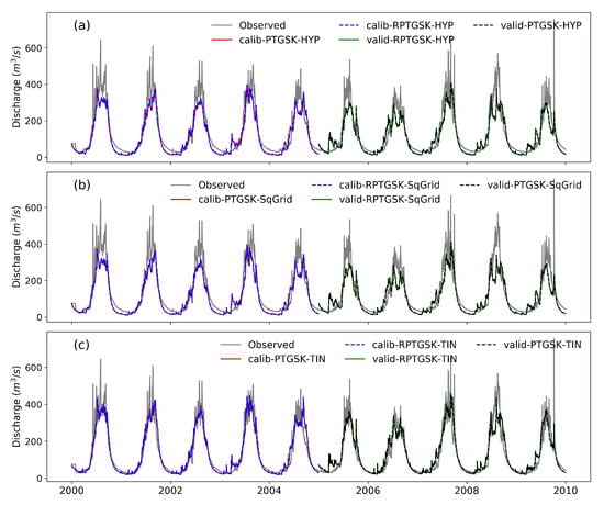
Figure 6.
Observed and simulated discharge from different models under the two radiation models i.e., PTGSK and RPTGSK for the discretizations, i.e., hypsography (a), square grid (b), and traingulated irregular network (c). In the figures legends, “Calib” and “valid” represent model calibration and validation, respectively.
Low flow simulations are relatively well captured by PTGSK-TIN and RPTGSK-TIN as compared to the other models. Modeled discharge during pre-monsoon season from all models was higher than observation, which is caused by the positive biases in the WFDEI precipitation during this season [10]. From the daily simulated hydrograph presented in the Figure 6, it can be seen that there is no notable difference in the simulated discharge from the model with and without using the imputed radiation.
Effect of the catchment discretization methods and radiation algorithms on model performance was further evaluated using NSE and LnNSE (Figure 7). The NSE and the LnNSE functions are a pair of conflicting objective functions, where the NSE function evaluates the ability to reproduce all stream flows, but it is known to be biased to predict peak flows [23], while the LnNSE function emphasizes low flows [62]. The model efficiency metrics were computed for each hydrologic year constituting the validation period. As such, each factor had 10 samples with a total size of 60 samples (two radiation algorithms and three discretization types). For model efficiency under high-flow condition as estimated using the raw-data (NSE) (Figure 7a), a more significant difference in model efficiency was observed between the catchment discretization types as compared to the radiation algorithms. The intercomparison between discretized models shows that TIN was superior to both the square grid cells (SqGrid) and the elevation bands (i.e., HYP), while HYP has yielded better result as compared to SqGrid. A similar order of performance between the three catchment discretization types was observed under the two radiation algorithms. Although a slight improvement was observed in SqGrid as a result of using RPTGSK against PTGSK, a slight deterioration in model performance was observed when using HYP and TIN with RPTGSK. A superior result was also obtained in model performance during low-flow conditions (LnNSE) when using TIN as compared to other catchment discretization types (Figure 7b). Unlike to the result obtained using NSE, a relatively better simulation result was obtained under SqGrid than HYP when assessed using LnNSE. No significant difference in LnNSE was also observed between the results obtained from PTGSK and RPTGSK.
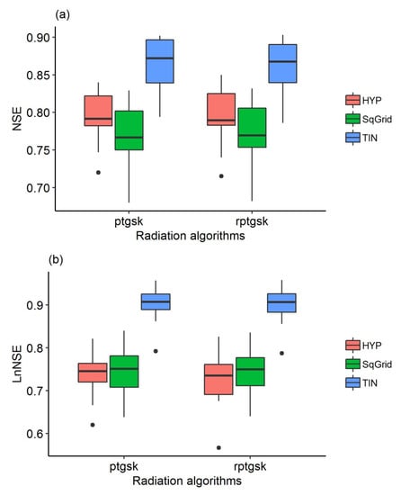
Figure 7.
Model efficiency during the high-flow (a) and low-flow (b) conditions under three catchment discretization types, i.e., elevation bands (HYP), square grids (SqGrid), and TIN as well as under two radiation algorithms (with (RPTGSK) and without (PTGSK) corrections based on certain terrain parameters.
3.3. Effects of Imputed Radiation on Snow Simulations
Results presented in the previous sections show that RPTGSK-TIN and PTGSK-TIN performed better than the remaining models. Therefore, these models were selected for snow cover analysis and validation of their snow cover simulations through comparison against the MODIS snow product. Figure 8a demonstrates monthly average percentage of snow cover area from MODIS, PTGSK-TIN, and RPTGSK-TIN. MODIS observations and model simulations show higher percentage of snow cover area during winter periods (January–April). The observed time series with strong seasonality in snow cover are adequately represented with both models. However, simulated values tend to underestimate the observed values during the low snow cover period i.e., June–October. To find the agreement between the model simulation and MODIS, monthly correlation coefficients were calculated. Highest monthly correlation coefficients based on five years (2005–2009) simulation were observed between MODIS and RPTGSK-TIN snow during February (0.85), April (0.76), and May (0.63). Similar to RPTGS-TIN, highest correlation coefficients between PTGSK-TIN and MODIS were observed during February (0.75), April (0.64), and May (0.60). Negative correlation coefficients between MODIS and both models were observed during December and January. It is also important to note that the snow simulations from both models at the beginning of 2006 was near to zero. However, we can see such abrupt decrease in snow cover at the beginning of every years. It is due to the fact that in the gamma snow model, snow cover area from the model start accumulating from the beginning of the calendar year.
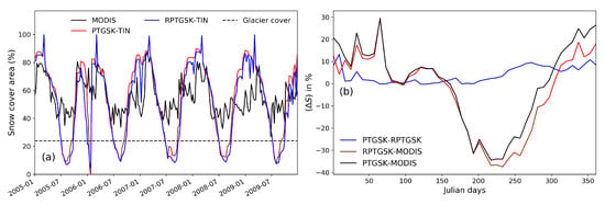
Figure 8.
(a) Catchment scale 8-day maximum snow cover area (%) from MODIS, PTGSK-TIN, and RPTGSK-TIN. (b) Snow cover area percentage differences between PTGSK-TIN and RPTGSK-TIN (blue), RPTGSK-TIN and MODIS (red), and PTGSK-TIN and MODIS (black).
Snow cover areas from the MODIS during July, August, and September are higher than from the models. Higher percentage of snow cover from MODIS might be connected to the fact that MODIS does not distinguish between snow and glacier, and considers both as a snow cover. Unlike to MODIS observations, glacier area is not simulated in Gamma snow, hence lower percentage of snow cover area during the snow ablation periods was found. The other possible source of uncertainty in the snow observations from MODIS during this period is related to cloud cover, which is obviously very high during monsoon period as mention by Riggs et al. [63].
Figure 8b shows five year daily average snow cover area percentage differences between the two models simulations and with the MODIS. With the implementation of imputed radiation in to the models, significant differences were observed in snow simulation. With in the two model snow simulation, highest differences (up to 12%) were observed during the winter season. However, when compared with the MODIS the difference was up to 35%. This highest difference between MODIS and model simulation is due to the fact that MODIS is not able to differentiate between snow and glaciers but from the model it only simulate snow. Observed highest peak snow from models are related with the model forcing datasets particularly precipitation. Because we have used relatively coarse forcing datasets. Therefore, when it interpolate it might give precipitation to the grid/TINs with no precipitation.
Figure 9 presents monthly CSI values of snow cover calculated from MODIS and model results for the simulation periods 2005 to 2009. The numbers inside the box represents median CSI values. The highest CSI from both models was obtained during pre-monsoon season (March–June) and the CSI score from both models are nearly the same. Median CSI score for both models during the pre-monsoon was approximately 0.75, indicating that 75% of the simulated snow from PTGSK-TIN and RPTGSK-TIN matches the remote observations. Similar to the correlation coefficient values, the lowest CSI scores were observed during the winter and monsoon periods. There is a slight increase in CSI score for RPTGSK-TIN simulation relative to PTGSK-TIN during June, July, and August.
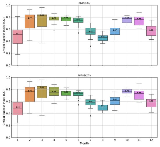
Figure 9.
Monthly Critical Success Index calculated for models (PTGSK-TIN, and RPTGSK-TIN). Numbers inside boxplot represent median value.
The scatterplots between the 8-day snow cover area fraction from models and MODIS in different elevations are shown in Figure 10. As can be seen from this figure, the topography seems to have a dominating effect on snow cover distribution. In the elevation ranges up to 3000 m asl, very few snow events were detected from both models and almost no snow events were detected from the MODIS. The ranges from 3000 to 6000 m asl experience greater snow coverage, whose spatial distribution is relatively better captured by both data sets. A slightly higher correlation coefficient between MODIS and RPTGSK-TIN simulation was observed as compared to PTGSK-TIN (Figure 10). During the snow ablation period, the high mountain ranges (>6000 m asl) have permanent glaciers which are not simulated by Gamma snow but detected in MODIS giving lower correlation coefficients for both models.
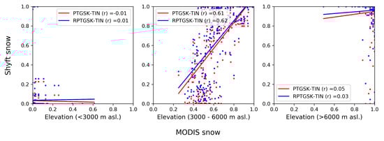
Figure 10.
Scatterplot between MODIS derived snow and models (PTGSK-TIN and RPTGSK-TIN) for each altitudinal zone. In each plot “r” represent correlation coefficient.
4. Discussion
The basic assumption in this study was that different model discretization methods were the reason for the differences in model performance. The results obtained through a variety of statistical models analysis undeniably follow the catchment discretization methods. We found all six models performed well (NSE > 0.75) for both calibration and validation. In general, all discretization methods provide an excellent representation of the general flow pattern and the overall water balance, while maintaining the significant interannual variability satisfying. As higher efficiency discharge simulation from the TIN-based discretized models also means higher efficiency snow cover simulation, only RPTGSK-TIN and PTGSK-TIN are used for snow cover simulation.
The predicted hydrographs for the calibration/validation, shown in Figure 6, confirm that the overall hydrograph pattern is predicted quite well by all models. Similar to the previous studies in [14,64,65], better performance was observed for the models with TINs. The poor performance of the grid-based models are partly attributed to complex topography of the region and the associated difference in distribution of land area (Figure 11). According to the NSE and the LnNSE of the outlet discharge, the rank of discretized model efficiency, in descending order, is TIN, HYP, and SqGrid models both in the calibration and validation periods. SqGrid are better than HYP when assessed using LnNSE. Theoretically, the ability to account for spatial variability of meteorological forcing and physical features within a catchment should lead to better simulations [66]. However, similar to the prior studies by Reed et al. [67] and Smith et al. [68], we found that grid based distributed modeling approaches do not always provide improved discharge simulation compared to hypsography discretized conceptual models. As presented by Birhanu et al. [69] and Xu et al. [70], land cover types are highly dependent on elevation change, thus the catchment discretized by the elevation bands represent catchment better than the grid. As a result, in our study, better land representation in hypsography-based models results in higher model efficiency compared to grid based model.
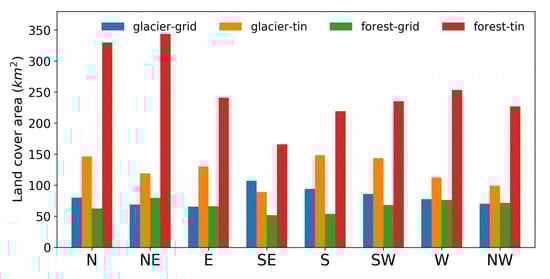
Figure 11.
Land type distribution in Marsyangdi_2 river catchment from TIN and grid.
The Delaunay triangulation is a widely appreciated and investigated mathematical model used to represent the topography and is highly efficient for building TINs. Vivoni [65] mention that in the regions of high terrain variability, the catchment discretized with TINs can be modeled more precisely due to higher flexibility of the mesh. The areas with little variation in topography are represented by larger triangles and the areas with more variation are represented by smaller ones leading to better representation of the ground shape [15]. Figure 11 shows the distribution of land cover area in grid and TIN. Remarkable differences are seen for the glacier and forest cover area. Another reason for finding higher amount of forest area in the TIN-based discretization was because of assuming more vegetation types as a forest. Therefore higher efficiencies from the models with TIN are also attributed to the better representation of land cover area. One of the most useful characteristics of a TIN for hydrologic system is the ability to define stream in terms of triangle boundary segments. This allows a more continuous description of stream paths and networks in conjunction with the topography. By comparison, grid data tend to produce zig-zag meandering paths for stream on upslope portions of a watershed [64]. As indicated by Jenness et al. [71], Raster datasets, such as DEMs and surface-area grids, are inherently less accurate and precise than vector data sets such as TINs and polygons. Grid values do not reflect the actual measurements. The grid model is not adaptive, and although TINs will naturally represent an area with detailed relief information with a denser triangle pattern than area with a smoother relief, grids will be far less flexible to cope with variable levels of details [15].
The overall performance of the CSI estimated by the PTGSK-TIN is somewhat reduced compared to RPTGSK-TIN 5 years (2005–2009) simulation runs for the Marsyangdi_2 catchment as expected (Figure 8 and Figure 9). However, biases in catchment average snow cover area from PTGSK-TIN and RPTGSK-TIN are less then 1%. The central estimate (median) from RPTGSK-TIN is slightly better (Figure 9; July-August-September) than PTGSK-TIN for studied catchment, giving better representation of observed simulated snow cover area.
Significant differences between snow simulation were observed by the implementation of imputed radiation algorithm in to the Shyft. Differences were higher during the winter season (i.e., up to 12%). When we compared with the MODIS snow, the difference between the simulation and the model as compared with MODIS was found to be higher (up to 4%) during summer. This is because MODIS does not distinguish between snow and ice, but models only simulate snow. With the imputed radiation, notable differences were also observed in evapotranspiration (see: Table 6). As seen in Figure 12A, unlike to Figure 12B, radiation is not distributed uniformly, and more radiation was received by south-east and south-west aspect. Lower percentage of the radiation is distributed to the Northern aspect. It should be noted that small percentage of higher radiations are also seen on northern aspect, but similar to the study by Burtscher [72], higher radiation in the northern aspect is because of the high elevation area there.
Table 6.
Annual (2005) water balance components for Marshyangdi_2 river catchment.
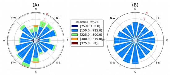
Figure 12.
Distribution of daily average (2005) WFDEI radiation with respect to aspect (A) Interpolated translate radiation; (B) Interpolated radiation radiation.
Although the overall efficiencies in terms of CSI and NSE are not significantly different (Figure 6 and Figure 8), effect of implemented imputed radiation can be clearly seen in water balance components (Table 6). As seen in Figure 12A, a lower percentage of radiation is distributed towards the East–South aspect resulting in lowering the total glacier melt. Furthermore, the lower percentage of evaporation is also observed for the model with imputed radiation and could be caused by reduced radiation.
5. Conclusions
This study was focused on evaluation of the effect of three catchment discretization approaches: hypsography (HYP), square grid (SqGrid), and TIN on hydrological model simulation results, i.e., streamflow and snow cover. Different discretization methods are not compared for snow cover in this paper. Use of two different algorithms for imputed radiation and its impact on model simulation results was also assessed. The different configurations were successfully applied to discharge simulation in Marsyangdi_2 river catchment. Generally, a good agreement between the observed and modeled discharge was obtained from the different configurations. The model simulation results based on the different discretization approaches, i.e., TIN, HYP, and SqGrid, were evaluated using graphical and certain efficiency metrics and they have shown a decreasing order of performance.
Selection of the catchment discretization methods depends upon the availability of computational resources and acceptable model efficiency. Regular SqGrid models are less flexible, but offer higher speed, lower memory requirements, and easier implementation algorithms as most important assets, making them to be preferred when the studied area is more flat. For area with high relief, typical for hydrological modeling, TINs are a priori the preferred option.
Direct use of radiation from WFDEI is a good option for hydrological modeling in a catchment. Snow simulation results did not show any changes when using imputed radiation; the snow cover determined by the direct use of radiation approach in the high mountain region does not represent the real snow cover area. Additional work is still needed to test and validate the suitability of snow simulation determination at different spatial and temporal scales using imputed radiation. Snow simulation with the models with TIN and imputed radiation should also be validated by other models with a much wider range of terrain types.
Finally, our study area represents a very complex regime in the central Himalayas, Nepal, and the results are encouraging. The findings presented in the paper provide valuable new regional knowledge and contribution in the catchment hydrology of the Himalayan region. The TIN-based models are particularly suited to the Himalayan catchments with steep descent/ascent because of the uniform slope along each triangle facet. With including values of TIN and the bias corrected WFDEI dataset is the best performing methods for the discharge simulation and water resource-related model application in the Himalayan region. This methods can be used in the other Himalayan catchments. If the study is constrained by time and computational memory, hypsography-based discretization methods represent a better option than the grid-based method.
Author Contributions
B.C.B., O.S. (Olga Silantyeva), A.T.T., and J.F.B. designed and performed the anlaysis. B.C.B. wrote the manuscript. J.F.B. supervised the study. S.H., O.S. (Ola Skavhaug), and O.S. (Olga Silantyeva) implemented the relevant algorithms in Shyft. All authors revised the manuscript. All authors have read and agreed to the published version of the manuscript.
Funding
This research received no external funding.
Acknowledgments
We are thankful to entire MODIS science team and NASA providing a massive data. This work was conducted within the Strategic Research Initiative “Land Atmosphere Interaction in Cold Environments” (LATICE) of the University of Olso and partially supported through the Norwegian Research Council’s INDNOR program under the Hydrologic sensitivity to Cryosphere-Aerosol interaction in Mountain Processes (HyCAMP) project (NFR no. 222195). Last but not least, we would like to thanks all three anonymous reviewer for their constructive thought and comments during the revision of this paper.
Conflicts of Interest
The authors declare no conflict of interest.
References
- Xu, C.Y. Climate change and hydrologic models: A review of existing gaps and recent research developments. Water Resour. Manag. 1999, 13, 369–382. [Google Scholar] [CrossRef]
- Li, H.; Zhang, Y.; Zhou, X. Predicting surface runoff from catchment to large region. Adv. Meteorol. 2015, 2015, 720967. [Google Scholar] [CrossRef]
- Martinec, J.; Rango, A.; Major, E. The Snowmelt-Runoff Model (SRM) User’s Manual; NASA Reference Publication (RP): Washington, DC, USA, 1983; Available online: https://jornada.nmsu.edu/bibliography/08-023.pdf (accessed on 17 August 2020).
- Halwatura, D.; Najim, M. Application of the HEC-HMS model for runoff simulation in a tropical catchment. Environ. Model. Softw. 2013, 46, 155–162. [Google Scholar] [CrossRef]
- Nepal, S.; Krause, P.; Flügel, W.A.; Fink, M.; Fischer, C. Understanding the hydrological system dynamics of a glaciated alpine catchment in the Himalayan region using the J2000 hydrological model. Hydrol. Process. 2014, 28, 1329–1344. [Google Scholar] [CrossRef]
- Burkhart, J.F.; Matt, F.N.; Helset, S.; Sultan Abdella, Y.; Skavhaug, O.; Silantyeva, O. Shyft v4.8: A Framework for Uncertainty Assessment and Distributed Hydrologic Modelling for Operational Hydrology. Geosci. Model Dev. Discuss. 2020, 2020, 1–29. [Google Scholar] [CrossRef]
- Kolberg, S.; Rue, H.; Gottschalk, L. A Bayesian spatial assimilation scheme for snow coverage observations in a gridded snow model. Hydrol. Earth Syst. Sci. 2006, 10, 369–381. [Google Scholar] [CrossRef]
- Bell, V.; Kay, A.; Jones, R.; Moore, R. Use of a grid-based hydrological model and regional climate model outputs to assess changing flood risk. Int. J. Climatol. J. R. Meteorol. Soc. 2007, 27, 1657–1671. [Google Scholar] [CrossRef]
- Hegdahl, T.J.; Tallaksen, L.M.; Engeland, K.; Burkhart, J.F.; Xu, C.Y. Discharge sensitivity to snowmelt parameterization: A case study for Upper Beas basin in Himachal Pradesh. Hydrol. Res. 2016, 47, 683–700. [Google Scholar] [CrossRef]
- Bhattarai, B.C.; Burkhart, J.F.; Tallaksen, L.M.; Xu, C.Y.; Matt, F.N. Evaluation of global forcing datasets for hydropower inflow simulation in Nepal. Hydrol. Res. 2020, 51, 202–225. [Google Scholar] [CrossRef]
- Martinec, J.; Rango, A.; Roberts, R. Snowmelt Runoff Model (SRM) User’s Manual Agricultural Experiment Station Special Report 100 College of Agriculture and Home Economics; Special Re, Ed.; College of Agriculture and Home Economics: Stockton, CA, USA, 2008. [Google Scholar]
- Pradhananga, N.S.; Kayastha, R.B.; Bhattarai, B.C.; Adhikari, T.R.; Pradhan, S.C.; Devkota, L.P.; Shrestha, A.B.; Mool, P.K. Estimation of discharge from Langtang River basin, Rasuwa, Nepal, using a glacio-hydrological model. Ann. Glaciol. 2014, 55, 223–230. [Google Scholar] [CrossRef]
- Bhattarai, B.C.; Regmi, D. Impact of Climate Change on Water Resources in View of Contribution of Runoff Components in Stream Flow: A Case Study from Langtang Basin, Nepal. J. Hydrol. Meteorol. 2015, 9, 74–84. [Google Scholar] [CrossRef]
- Singh, V.P.V.P.; Fiorentino, M. Geographical Information Systems in Hydrology; Springer: Dordrecht, The Netherlands, 1996; p. 446. [Google Scholar]
- De Wulf, A.; Constales, D.; Nuttens, T.; Stal, C. Grid models versus TIN: Geometric accuracy of multibeam data processing. In Proceedings of the Hydro12, Rotterdam, The Netherlands, 13–15 November 2012. [Google Scholar]
- Freer, J.; McDonnell, J.; Beven, K.; Brammer, D.; Burns, D.; Hooper, R.P.; Kendal, C. Topographic controls on subsurface storm flow at the hillslope scale for two hydrologically distinct small catchments. Hydrol. Process. 1997, 11, 1347–1352. [Google Scholar] [CrossRef]
- Woods, R.A.; Sivapalan, M.; Robinson, J.S. Modeling the spatial variability of subsurface runoff using a topographic index. Water Resour. Res. 1997, 33, 1061–1073. [Google Scholar] [CrossRef]
- Diffenbaugh, N.S.; Scherer, M.; Ashfaq, M. Response of snow-dependent hydrologic extremes to continued global warming. Nat. Clim. Chang. 2013, 3, 379–384. [Google Scholar] [CrossRef]
- Lutz, A.F.; Immerzeel, W.W.; Shrestha, A.B.; Bierkens, M.F.P. Consistent increase in High Asia’s runoff due to increasing glacier melt and precipitation. Nat. Clim. Chang. 2014, 4, 587–592. [Google Scholar] [CrossRef]
- Sam, L.; Bhardwaj, A.; Kumar, R.; Buchroithner, M.F.; Martín-Torres, F.J. Heterogeneity in topographic control on velocities of Western Himalayan glaciers. Sci. Rep. 2018, 8, 12843. [Google Scholar] [CrossRef]
- Braakmann-Folgmann, A.; Donlon, C. Estimating snow depth on Arctic sea ice using satellite microwave radiometry and a neural network. Cryosphere 2019, 13, 2421–2438. [Google Scholar] [CrossRef]
- Parajka, J.; Holko, L.; Kostka, Z.; Blöschl, G. MODIS snow cover mapping accuracy in a small mountain catchment-comparison between open and forest sites. Hydrol. Earth Syst. Sci. 2012, 16, 2365–2377. [Google Scholar] [CrossRef]
- Teweldebrhan, A.; Burkhart, J.F.; Schuler, T.V. Parameter uncertainty analysis for an operational hydrological model using residual-based and limits of acceptability approaches. Hydrol. Earth Syst. Sci. 2018, 22, 5021–5039. [Google Scholar] [CrossRef]
- Allen, R.G.; Trezza, R.; Tasumi, M. Analytical integrated functions for daily solar radiation on slopes. Agric. For. Meteorol. 2006, 139, 55–73. [Google Scholar] [CrossRef]
- Li, H.; Wang, Z.; He, G.; Man, W. Estimating Snow Depth and Snow Water Equivalence Using Repeat-Pass Interferometric SAR in the Northern Piedmont Region of the Tianshan Mountains. J. Sens. 2017, 2017, 8739598. [Google Scholar] [CrossRef]
- Hall, D.K.; Riggs, G.A.; Salomonson, V.V.; DiGirolamo, N.E.; Bayr, K.J. MODIS snow-cover products. Remote Sens. Environ. 2002, 83, 181–194. [Google Scholar] [CrossRef]
- Zhang, G.; Xie, H.; Yao, T.; Liang, T.; Kang, S. Snow cover dynamics of four lake basins over Tibetan Plateau using time series MODIS data (2001–2010). Water Resour. Res. 2012, 48. [Google Scholar] [CrossRef]
- Urraca, R.; Gracia-Amillo, A.M.; Huld, T.; Martinez-de Pison, F.J.; Trentmann, J.; Lindfors, A.V.; Riihelä, A.; Sanz-Garcia, A. Quality control of global solar radiation data with satellite-based products. Sol. Energy 2017, 158, 49–62. [Google Scholar] [CrossRef]
- Fan, Y.; Clark, M.; Lawrence, D.M.; Swenson, S.; Band, L.E.; Brantley, S.L.; Brooks, P.D.; Dietrich, W.E.; Flores, A.; Grant, G.; et al. Hillslope Hydrology in Global Change Research and Earth System Modeling. Water Resour. Res. 2019, 55, 1737–1772. [Google Scholar] [CrossRef]
- Priestley, C.H.B.; Taylor, R.J. On the Assessment of Surface Heat Flux and Evaporation Using Large-Scale Parameters. Mon. Weather Rev. 1972, 100, 81–92. [Google Scholar] [CrossRef]
- Lambert, A.O. Catchment models based on ISO-functions. J. Inst. Water Eng. 1972, 26, 413–422. [Google Scholar]
- Kirchner, J.W. Catchments as simple dynamical systems: Catchment characterization, rainfall-runoff modeling, and doing hydrology backward. Water Resour. Res. 2009, 45. [Google Scholar] [CrossRef]
- DeWalle, D.R.; Rango, A. Principles of Snow Hydrology; Cambridge University Press: Cambridge, UK, 2008. [Google Scholar] [CrossRef]
- Hock, R. Temperature index melt modeling in mountain areas. J. Hydrol. 2003, 282, 104–115. [Google Scholar] [CrossRef]
- Bajracharya, S.R.; Maharjan, S.B.; Shrestha, F.; Bajracharya, O.; Baidya, S. Glacier Status in Nepal and Decadal Change from 1980 to 2010 Based on Landsat Data; Technical Report; International Centre for Integrated Mountain Development: Kathmandu, Nepal, 2014. [Google Scholar]
- Bhattarai, B.C.; Burkhart, J.F.; Stordal, F.; Xu, C.Y. Aerosol Optical Depth Over the Nepalese Cryosphere Derived From an Empirical Model. Front. Earth Sci. 2019, 7, 178. [Google Scholar] [CrossRef]
- Nayava, J.L. Heavy Monsoon Rainfall in Nepal. Weather 1974, 29, 443–450. [Google Scholar] [CrossRef]
- Kripalani, R.H.; Sontakke, N.A. Rainfall variability over Bangladesh and Nepal: Comparison and connections with features over India. Int. J. Climatol. 1996, 16, 689–703. [Google Scholar] [CrossRef]
- Adhikari, D. Hydropower Development in Nepal. NRB Econ. Rev. 2006, 18, 70–94. [Google Scholar]
- Weedon, G.P.; Balsamo, G.; Bellouin, N.; Gomes, S.; Best, M.J.; Viterbo, P. The WFDEI meteorological forcing data set: WATCH Forcing Data methodology applied to ERA-Interim reanalysis data. Water Resour. Res. 2014, 50, 7505–7514. [Google Scholar] [CrossRef]
- Raimonet, M.; Oudin, L.; Thieu, V.; Silvestre, M.; Vautard, R.; Rabouille, C.; Le Moigne, P. Evaluation of gridded meteorological datasets for hydrological modeling. J. Hydrometeorol. 2017, 18, 3027–3041. [Google Scholar] [CrossRef]
- Essou, G.R.; Sabarly, F.; Lucas-Picher, P.; Brissette, F.; Poulin, A. Can precipitation and temperature from meteorological reanalyses be used for hydrological modeling? J. Hydrometeorol. 2016, 17, 1929–1950. [Google Scholar] [CrossRef]
- Gurung, D.; Amarnath, G.; Khun, S.; Shrestha, B. Snow-Cover Mapping and Monitoring in the Hindu Kush-Himalayas; ICIMOD: Kathmandu, Nepal, 2011. [Google Scholar]
- Stroeve, J.C.; Box, J.E.; Haran, T. Evaluation of the MODIS (MOD10A1) daily snow albedo product over the Greenland ice sheet. Remote Sens. Environ. 2006, 105, 155–171. [Google Scholar] [CrossRef]
- Li, H.; Li, X.; Xiao, P. Impact of Sensor Zenith Angle on MOD10A1 Data Reliability and Modification of Snow Cover Data for the Tarim River Basin. Remote Sens. 2016, 8, 750. [Google Scholar] [CrossRef]
- Williamson, S.N.; Anslow, F.S.; Clarke, G.K.C.; Gamon, J.A.; Jarosch, A.H.; Hik, D.S. Spring warming in Yukon mountains is not amplified by the snow albedo feedback. Sci. Rep. 2018, 8, 9000. [Google Scholar] [CrossRef]
- Rittger, K.; Painter, T.H.; Dozier, J. Assessment of methods for mapping snow cover from MODIS. Adv. Water Resour. 2013, 51, 367–380. [Google Scholar] [CrossRef]
- Toure, A.M.; Reichle, R.H.; Forman, B.A.; Getirana, A.; Lannoy, G.J.M.D. Assimilation of MODIS Snow Cover Fraction Observations into the NASA Catchment Land Surface Model. Remote Sens. 2018, 10, 316. [Google Scholar] [CrossRef] [PubMed]
- Muhammad, S.; Thapa, A. A combined Terra/Aqua MODIS snow-cover and RGI6. 0 glacier product (MOYDGL06) for the High Mountain Asia between 2002 and 2018. Earth Syst. Sci. Data 2020, 12, 345–356. [Google Scholar] [CrossRef]
- Arino, O.; Perez, J.R.; Kalogirou, V.; Defourny, P.; Achard, F. GlobCover 2009; ESA/ESA Globcover 2005 Project, Led by MEDIAS-France/POSTEL Image: © ESA/ESA Globcover 2005 Project, Led by MEDIAS-France/POSTEL 2010; Available online: http://due.esrin.esa.int/page_globcover.php (accessed on 17 August 2020).
- Van Zyl, J.J. The Shuttle Radar Topography Mission (SRTM): A breakthrough in remote sensing of topography. Acta Astronaut. 2001, 48, 559–565. [Google Scholar] [CrossRef]
- Akram, F.A.; Rasul, M.R.; Khan, M.K.; Amir, M. Automatic Delineation of Drainage Networks and Catchments using DEM data and GIS Capabilities: A case study. In Proceedings of the 18 th Australasian Fluid Mechanics Conference, Launceston, Australia, 3–7 December 2012. [Google Scholar]
- Field, D.A. Laplacian smoothing and Delaunay triangulations. Commun. Appl. Numer. Methods 1988, 4, 709–712. [Google Scholar] [CrossRef]
- Hjelle, Ø.; Dæhlen, M. Triangles and Triangulations. In Triangulations and Applications; Springer: Berlin/Heidelberg, Germany, 2006; pp. 1–21. [Google Scholar] [CrossRef]
- Vivoni, E.R.; Ivanov, V.Y.; Bras, R.L.; Entekhabi, D. Generation of Triangulated Irregular Networks Based on Hydrological Similarity. J. Hydrol. Eng. 2004, 9, 288–302. [Google Scholar] [CrossRef]
- Silantyeva, O.; Burkhart, J.F.; Bhattarai, B.C.; Skavhaug, O.; Helset, S. Operational hydrology in highly steep areas: Evaluation of tin-based toolchain. In Proceedings of the EGU Meeting, EGU General Assembly Conference Abstracts, Vienna, Austria, 4–8 May 2020; p. 8172. Available online: https://meetingorganizer.copernicus.org/EGU2020/EGU2020-8172.html?EGUSphere (accessed on 17 August 2020).
- Duan, Q.; Sorooshian, S.; Gupta, V. Effective and efficient global optimization for conceptual rainfall-runoff models. Water Resour. Res. 1992, 28, 1015–1031. [Google Scholar] [CrossRef]
- Nash, J.E.; Sutcliffe, J.V. River flow forcasting through conceptural models part {I-A} discussion of principles. J. Hydrol. 1970, 10, 282–290. [Google Scholar] [CrossRef]
- Krause, P.; Boyle, D.P.; Bäse, F. Comparison of different efficiency criteria for hydrological model assessment. Adv. Geosci. 2005, 5, 89–97. [Google Scholar] [CrossRef]
- Schaefer, J.T. The Critical Success Index as an Indicator of Warning Skill. Weather Forecast. 1990, 5, 570–575. [Google Scholar] [CrossRef]
- AghaKouchak, A.; Mehran, A. Extended contingency table: Performance metrics for satellite observations and climate model simulations. Water Resour. Res. 2013, 49, 7144–7149. [Google Scholar] [CrossRef]
- Huo, J.; Liu, L. Evaluation Method of Multiobjective Functions’ Combination and Its Application in Hydrological Model Evaluation. Comput. Intell. Neurosci. 2020, 2020, 8594727. [Google Scholar] [CrossRef] [PubMed]
- Riggs, G.; Hall, D.K. Reduction of cloud obscuration in the MODIS snow data product. In Proceedings of the 59th Eastern Snow Conference, Stowe, VT, USA, 5–7 June 2002; Volume 5. [Google Scholar]
- DeVantier, B.A.; Feldman, A.D. Review of GIS Applications in Hydrologic Modeling. J. Water Resour. Plan. Manag. 1993, 119, 246–261. [Google Scholar] [CrossRef]
- Vivoni, E.R. Hydrologic Modeling Using Triangulated Irregular Networks: Terrain Representation, Flood Forecasting and Catchment Response. Ph.D. Thesis, Massachusetts Institute of Technology, Cambridge, MA, USA, 2003. [Google Scholar]
- Brirhet, H.; Benaabidate, L. Comparison of Two Hydrological Models (Lumped and Distributed) over a Pilot Area of the Issen Watershed in the Souss Basin, Morocco. Eur. Sci. J. ESJ 2016, 12, 347. [Google Scholar] [CrossRef][Green Version]
- Reed, S.; Koren, V.; Smith, M.; Zhang, Z.; Moreda, F.; Seo, D.J.; DMIP Participants. Overall distributed model intercomparison project results. J. Hydrol. 2004, 298, 27–60. [Google Scholar] [CrossRef]
- Smith, M.B.; Seo, D.J.; Koren, V.I.; Reed, S.M.; Zhang, Z.; Duan, Q.; Moreda, F.; Cong, S. The distributed model intercomparison project (DMIP): Motivation and experiment design. J. Hydrol. 2004, 298, 4–26. [Google Scholar] [CrossRef]
- Birhanu, L.; Hailu, B.T.; Bekele, T.; Demissew, S. Land use/land cover change along elevation and slope gradient in highlands of Ethiopia. Remote Sens. Appl. Soc. Environ. 2019, 16, 100260. [Google Scholar] [CrossRef]
- Xu, E.; Zhang, H.; Yao, L. An Elevation-Based Stratification Model for Simulating Land Use Change. Remote Sens. 2018, 10, 1730. [Google Scholar] [CrossRef]
- Jenness, J.S. Calculating landscape surface area from digital elevation models. Wildl. Soc. Bull. 2004, 32, 829–839. [Google Scholar] [CrossRef]
- Burtscher, M. Effects of living at higher altitudes on mortality: A narrative review. Aging Dis. 2014, 5, 274–280. [Google Scholar] [CrossRef]


© 2020 by the authors. Licensee MDPI, Basel, Switzerland. This article is an open access article distributed under the terms and conditions of the Creative Commons Attribution (CC BY) license (http://creativecommons.org/licenses/by/4.0/).