Article

Evaluation of LNAPL Behavior in Water Table Inter-Fluctuate Zone under Groundwater Drawdown Condition

by
Reza Azimi
1,
Abdorreza Vaezihir
1,*,
Robert J. Lenhard
2 and
S. Majid Hassanizadeh
3
1
Department of Earth Sciences, University of Tabriz, 29 Bahman Blvd., Tabriz 5166616471, Iran
2
San Antonio, TX 78253, USA
3
Department of Earth Sciences, Utrecht University, 3584 CD Utrecht, The Netherlands
*
Author to whom correspondence should be addressed.
Water 2020, 12(9), 2337; https://doi.org/10.3390/w12092337
Submission received: 20 July 2020 / Revised: 11 August 2020 / Accepted: 15 August 2020 / Published: 20 August 2020
(This article belongs to the Special Issue Subsurface Multiphase Flow and Contamination Remediation)

Abstract

:
We investigate the movement of LNAPL (light non-aqueous phase liquid) into and out of monitoring wells in an immediate-scale experimental cell. Aquifer material grain size and LNAPL viscosity are two factors that are varied in three experiments involving lowering and rising water levels. There are six monitoring wells at varying distances from a LNAPL injection point and a water pumping well. We established steady water flow through the aquifer materials prior to LNAPL injection. Water pumping lowered the water levels in the aquifer materials. Terminating water pumping raised the water levels in the aquifer materials. Our focus was to record the LNAPL thickness in the monitoring wells under transient conditions. Throughout the experiments, we measured the elevations of the air-LNAPL and LNAPL-water interfaces in the monitoring wells to obtain the LNAPL thicknesses in the wells. We analyze the results and give plausible explanations. The data presented can be employed to test multiphase flow numerical models.

1. Introduction

Groundwater contamination by petroleum products is a common problem in many industrialized areas as well as in oil producing countries. Gasoline (petro), diesel fuel, and crude oil are potential groundwater pollutants. As a group, they are commonly called light non-aqueous phase liquids (LNAPLs), which may exist in the subsurface in four forms: vapor phase in vadose zone pore spaces, vadose zone liquid residual LNAPL, free phase LNAPL in the water-unsaturated zone, and entrapped LNAPL globules above and below the water table [1,2,3]. Understanding the volume and underground distribution of these forms is essential for predicting potential groundwater contamination and for designing associated remediation cleanup programs.
Remediation of groundwater at LNAPL contaminated sites is still a complicated and challenging issue. Poor planning can increase the potential risk to public health and the environment. Over time, engineers and scientists have increased their knowledge of subsurface LNAPL behavior from laboratory experiments, field observations, and models. From older conceptions that considered LNAPL as pancakes on the surface of the water-saturated region to the current understanding that regard LNAPL as free, residual, and entrapped phases with varying degrees of saturation, significant progress has beenmade [4]. Understanding how all forms of LNAPL are distributed underground [5], along with its possible risk to human health and the environment [6], is essential for defining and developing an effective LNAPL cleanup strategy.
Groundwater table fluctuations can change the subsurface distribution of the different LNAPL phases [7,8,9]. As the water table rises or falls, free LNAPL may become entrapped or entrapped LNAPL may become free LNAPL, respectfully [10]. Further, in the dry seasons as the groundwater level drops, free LNAPL may become a residual form in the unsaturated zone as the bulk of the free LNAPL migrates downwards with the water table.
Initially, various researchers have predicted the relationship between the thickness of LNAPL observed in a monitoring well to its actual thickness in groundwater aquifers [11,12,13,14,15,16,17]. They found that the actual thickness of LNAPL in the subsurface is less than that in monitoring wells. They calculated the volume of LNAPL in the subsurface from the predicted LNAPL thickness in the subsurface and the subsurface porosity. Some assumed the LNAPL saturation was one minus the residual water saturation instead of one (completely LNAPL saturated). In either case, the LNAPL saturation was assumed to be constant with depth—the pancake model. Later, Farr et al. and Lenhard, Parker [18,19] showed that LNAPL saturations in the subsurface vary with depth and is a function of the LNAPL-water capillary pressure. They predicted the LNAPL-water capillary pressures from the depths (or elevations) of the air-LNAPL and LNAPL-water interfaces in a monitoring well, assuming vertical LNAPL movement has terminated, i.e., vertical equilibrium. From the LNAPL-water capillary pressures, LNAPL saturations as a function of depth were predicted using approaches by Parker et al. [20]. When the LNAPL saturations are summed over a vertical slice of the subsurface near the well, the LNAPL volume of the subsurface vertical slice (specific LNAPL volume) is predicted. Parker, Lenhard [21] developed an approach to estimate the LNAPL transmissivity, which predicts the rate at which LNAPL in a vertical slice may move into a monitoring well utilizing relations by Parker et al. [20]. The approaches in Farr et al., Lenhard, Parker and Parker, Lenhard [18,19,21] assume all LNAPL is mobile and capillary pressure-saturation relations are single valued (i.e., non-hysteretic). Parker, Lenhard. [21] further assume saturation-relative permeability relations are single valued (i.e., non-hysteretic). The equations developed by Farr et al. and Lenhard, Parker [18,19] are analytical expressions to calculate the specific LNAPL volume. The equations developed by Parker, Lenhard [21] are vertically integrated capillary pressure-saturation-relative permeability relations (constitutive relations) for implementation in two-dimensional numerical models for predicting quasi three-dimensional subsurface LNAPL behavior.
Parker, Lenhard and Lenhard, Parker [22,23] also modelled hysteretic capillary pressure-saturation-relative permeability relations for porous media containing LNAPL. They considered LNAPL entrapment by water imbibition saturation paths, which can occur wherever LNAPL is displaced by water. Parker et al. [24,25] modified the [21] vertically integrated constitutive relations to consider LNAPL entrapment by water and residual LNAPL following LNAPL drainage in the vadose zone. They developed equations for predicting the specific total, free, entrapped, and residual LNAPL saturations as well as for the LNAPL transmissivity of the free LNAPL. Because their equations only predicted the various specific LNAPL volumes, the distribution of the different LNAPL forms as a function of depth (elevation) was unknown. Later, Waddill et al. [26] developed equations for calculating the average entrapped and residual LNAPL saturations in the unsaturated and saturated zones. The average saturations were constant values over the respective elevations. Still later, Lenhard et al. [27] modified the hysteretic [22,23] constitutive relations to include elevation-specific residual LNAPL saturation. Charbeneau, Charbeneau et al. and Jeong, Charbeneau [28,29,30] utilized the earlier works of [21,24,25,26] in their predictive models.
To provide insights concerning subsurface LNAPL behavior and test predictive models, investigators conducted small- and intermediate-scale laboratory experiments and field investigations [7,8,10,31,32,33,34,35,36,37,38,39,40]. The works involved entrapment of LNAPL, the effect of water table fluctuations, assessing LNAPL recoverability, transient effects, and other aspects. In addition, investigators conducted multidimensional, multiphase simulations considering free, residual, and entrapped LNAPL [28,30,41,42,43] to predict subsurface LNAPL behavior.
The purpose of this paper is to provide additional insights concerning the movement of LNAPL into monitoring wells by experimentally investigating LNAPL behavior subject to a fluctuating water table in both coarse- and fine-grained aquifer materials. We also consider effects of LNAPL viscosity. Although some investigators have considered effects of water table fluctuations previously, our focus is on characterizing transient aspects of changing LNAPL thickness in monitoring wells. We measure the time-dependent changes of monitoring well LNAPL thickness in a laboratory 3D model. The data presented can be employed to test multiphase flow numerical models. In addition to the measured changes of water and NAPL elevations in monitoring wells with time at various positions, we provide LNAPL and porous medium properties, initial conditions, and boundary conditions. Modelers can utilize this wealth of data to conduct simulations with multiphase flow numerical models. Relevant van Genuchten or Brooks-Corey parameters can be found in the literature.

2. Material and Methods

2.1. Tank Description

The experiment involved a glass tank with approximate inner dimensions of 50 cm high, 70 cm wide, and 50 cm deep (see Figure 1). The packed aquifer material had approximate dimensions of 40 cm high, 50 cm wide, and 50 cm deep (i.e., the aquifer material packing was to a 40 cm height with the inlet water chamber being 12.5 cm wide and the outlet water chamber being 7.5 cm wide). A water pumping well was located at the center of the tank and six observation wells were located, as shown in Figure 1. All wells penetrated the aquifer materials to the base of the tank, had a diameter of 2 cm, and were screened 35 cm to prevent entry of aquifer material. Screening also prevented aquifer material from entering the inlet and outlet flow chambers of the tank.
Adjustable floats controlled the water levels in the inlet chamber, thereby manipulating the water flow rate through the sand. A 1-cm diameter drainage tube was used to control the water level in the outlet chamber. Further, an adjustable pump controlled pumping rates from the pumping well. To measure LNAPL (light non-aqueous phase liquid) thickness in the wells, a HERON Oil-Water Interface meter was used, which required the wells to have the 2 cm diameter. The interface meter measures air-water, air-LNAPL and LNAPL-water interface elevations with a precision of 0.1 cm.
A drop in water level near the pumping well was accomplished by pumping from the well. During the pumping period, the valve to the inlet chamber was kept open to maintain a constant water level in the inlet chamber with aid of the float. To restore the water level near the pumping well to its original level, pumping was stopped and the water flow from the inlet chamber was maintained.

2.2. Aquifer Material

We used glass beads as aquifer material to minimize effects of potential heterogeneities and anisotropy from packing the tank. Further, aquifer material grain size is more easily controlled with using glass beads. We used glass beads with a size range of 400 to 750 μm in diameter, for what we refer to as our coarse-grained aquifer material, and glass beads with a size range of <125 μm in diameter, for what we refer to as our fine-grained aquifer material. During our experiments with fine-grained aquifer material, we used glass beads with a size range of 400 to 750 μm as a ‘gravel pack’ around the wells. The water saturated hydraulic conductivities for the coarse- and fine-grained aquifer materials are 2.5 and 0.79 m/day, respectively. The dry bulk densities for the coarse- and fine-grained aquifer materials are 1620 and 1400 kg/m3, respectively.

2.3. LNAPL Properties

In order to study the effect of viscosity, we employed two different LNAPLs (crude oil and gas oil). The physical properties of these LNAPLs are listed in Table 1. The crude oil is Iranian Crude Oil and the gas oil is a refined product from the Shazand Refinery in central Iran. In order to visualize the gas oil in our experiments, we mixed the gas oil with “Blue Dispers BL” dye made by Alwan Company in Iran.

2.4. Injection of LNAPLs

LNAPL was injected into the aquifer materials between the observation well M1 and the pumping well (PW) (see Figure 1) with a 1-cm diameter tube. We used different protocols for the LNAPL injection based on the aquifer material. For the coarse-grained aquifer material, we injected the LNAPLs continuously at about 5 cm below aquifer material surface at a pressure head of approximately 10 cm. The LNAPLs migrated downwards spreading over and depressing the water capillary fringe. For the fine-grained aquifer material, we injected the LNAPL at the water table at a pressure head of approximately 25 cm. The volume of LNAPL injected in all cases was approximately 1500 cm3 (1.5 L).

3. Experiments

We performed three different experiments to study the behavior of LNAPL (light non-aqueous phase liquid) thickness in observation wells (Table 2). Two main factors were LNAPL type and grain size of the aquifer materials.
During the experiments, we measured the elevations of the air-LNAPL and LNAPL-water interfaces in the observation wells. For ease of following discussions, we employ abbreviations to refer to the thickness of LNAPL in the aquifer materials and wells, which are shown in Figure 2.

3.1. Experiment E1: Coarse Grain, Gas Oil

Prior to LNAPL injection, the water elevations in the inlet and outlet chambers were set at 23.1 and 22.1 cm, respectively. LNAPL injection was initiated after steady-state water flow conditions were established. The flow of water through the packed aquifer material was approximately 1.25 × 10⁻⁶ m3/s. 24 h after LNAPL injection was terminated, water was pumped from the pumping well at a rate of 5.6 × 10⁻⁶ m3/s for 102 min to cause a rapid drop in the groundwater table. After LNAPL injection and before water pumping, some LNAPL passed from the aquifer material into both the inlet and outlet chambers. There was a greater amount of LNAPL in the outlet chamber than the inlet chamber, which only had a minor amount. After water pumping was terminated, the groundwater level returned to its original level. Air-LNAPL (Zao) and LNAPL-water (Zow) interfaces were measured in the monitoring wells. The change of LNAPL thickness (Zo) in the monitoring wells following the start of water pumping is shown in Figure 3. For a better understanding of how LNAPL thickness (Zo) changed, Zao and Zow in the monitoring wells following the start of water pumping are shown in Figure 4 and Figure 5, respectively. Figure 6 schematically shows Zo in each monitoring well before pumping, immediately after pumping, and at the end of test (experiment).
At the onset of pumping (see Figure 3, time = 0), M1 and M6 had approximately the same Zo with M3 having a slightly greater thickness, which suggests there may be some heterogeneity in the packing because both M1 and M6 are closer to the LNAPL injection point than M3 (see Figure 1). Transient conditions existed during the experiment and ideally M3 should have a smaller LNAPL thickness than M1 and M6. Farther from the LNAPL injection point, M2 and M4 had similar LNAPL thicknesses, which is reasonable. The very small LNAPL thickness at M5 is also reasonable because it lies some distance upstream of the injection point. The greater the LNAPL thickness in a well typically indicates the LNAPL saturation will be higher in the aquifer next to it and some LNAPL will be contained in larger pore spaces.
During water pumping, the produced cone of depression is expected to be nonsymmetrical because of water flow from the inlet to outlet chambers. One would expect LNAPL to drain toward the bottom of the water depression. From Figure 4, it shows Zao decreased similarly for all monitoring wells, except for M1 which did not decline as much as the other monitoring wells. The explanation for the M1 Zao behavior is unclear, but may be attributed to the nonsymmetrical water depression from pumping. From Figure 5, Zow was different for each monitoring well because of the different Zo in each monitoring well initially and the effects from the pumping. From about 50 min to the end of pumping, the rate of decline in Zow was less for M1, M3, and M6, which are the closer wells to the pumping well, than for M2, M4, and M5. The rate of decline in Zow for M3 and M6, however, is slightly less than the decline in Zao, which means Zo is decreasing for those wells. The rate of decline in Zow for M2, M4, and M5, conversely, is slightly greater than the decline in Zao, which means Zo is increasing in those monitoring wells. Since the rate of decline in Zao for M1 is even less than the rate in other wells and the rate of decline in Zow is less than the Zao rate, Zo is increasing. Again, the behavior at M1 is unclear. Transient fluid flow is complicated. Because of the rates at which Zao and Zow declined due to water pumping, Zo slightly decreased in M3 and M6, but increased, sometimes significantly, in M1, M2, M4, and M5 at the termination of pumping. A plausible explanation for the increase in Zo at the end of pumping for M2, M4, and M5 could be the migration of LNAPL from the inlet and outlet chambers. The cone of depression from pumping would produce a gradient whereby LNAPL under slight positive pressures in the chambers would migrate to the aquifer material.
After pumping was terminated, Zao and Zow increased, as seen in Figure 4 and Figure 5, respectively, indicating rising water table. During pumping, LNAPL was migrating to the center of the water cone of depression at the pumping well. Following pumping, the mass of LNAPL near the pumping well will move upwards and outwards as the water table rises. As seen in Figure 5, the increase in Zow appears to be approaching a stable level in all of the monitoring wells when the experiment was terminated, but Zao was still increasing, indicating the LNAPL was still redistributing at the end of the experiment. Figure 3 shows that the increase in Zo in the monitoring wells is greater for wells closer to the pumping well. At the end of the experiment, the LNAPL thickness in all monitoring wells is greater than that at the onset of pumping (Figure 6). The difference in LNAPL thicknesses in the wells at the end of pumping and the end of the experiment may be also partly attributed to hysteresis in capillary pressure-saturation relations.

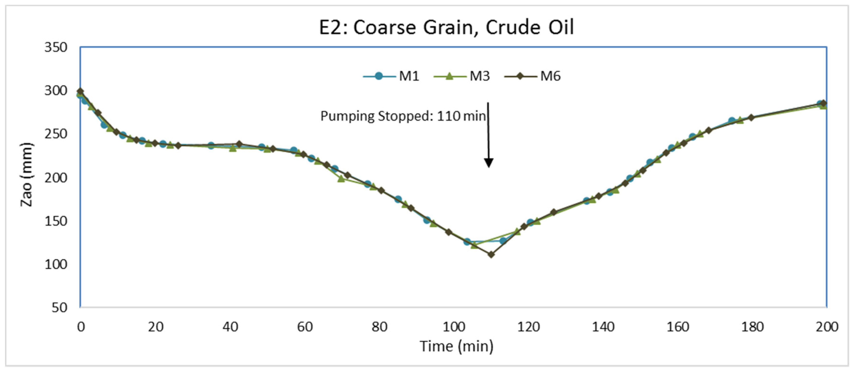
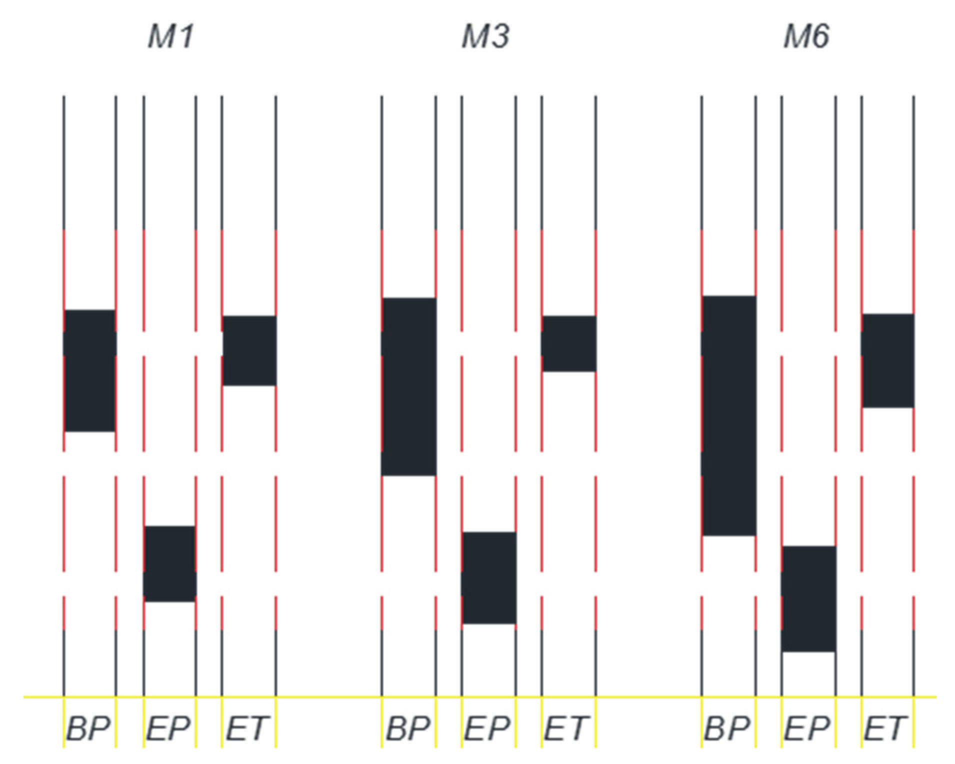
3.2. Experiment E2: Coarse Grain, Crude Oil

After repacking the tank with coarse-grained aquifer material and establishing water flow from the inlet to outlet chambers, we injected crude oil as the LNAPL. Packing the tank and establishing water flow followed similar procedures as for E1. The water elevation in the inlet and outlet chambers were set at 30.3 cm and 29.5 cm, respectively. The flow of water through the packed aquifer material was approximately 1 × 10⁻⁶ m3/s. Roughly 7 days after LNAPL injection, the water level was lowered via water pumping from the pumping well. Pumping continued for 110 min at a discharge rate of 4 × 10⁻⁶ m3/s. The pump was then turned off so that the water levels could return to pre-pumping elevations. At the beginning of pumping, M2, M4, and M5 did not have any LNAPL because they were farther from the injection point than M1, M3, and M6. In fact, no LNAPL entered M2, M4, and M5 at any time during E2. The higher viscosity of the crude oil relative to the gas oil caused the crude oil to migrate at a much slower rate than the gas oil. The LNAPL thicknesses (Zo) in monitoring wells M1, M3, and M6 during the experiment (E2) are shown in Figure 7. Figure 8 and Figure 9 show the elevation changes of Zao and Zow, respectively. In addition, we show Zo in M1, M3, and M6 before water pumping, immediately after pumping, and at the end of the experiment in Figure 10.
Prior to pumping (Figure 7, time = 0), LNAPL had entered only M1, M3, and M6. Although M1 is closer to the LNAPL injection point than M3 and M6, Zo is greater in M3 and M6. A possible explanation is that M1 is upgradient to the water flow, whereas M3 and M6 are downgradient from the injection point (Figure 1). The larger Zo in M6 is likely due to the fact that it is closer to the injection point than M3. Even after 7 days of LNAPL redistribution, transient flow conditions likely existed because of the high LNAPL viscosity.
Shortly after water pumping from the pumping well started, Figure 8 and Figure 9 show Zao and Zow in M1, M3, and M6 rapidly decreasing due to the lowering of the water table. The Zo in these monitoring wells (Figure 7), however, did not decline as rapidly because of the high LNAPL viscosity. The flow of LNAPL toward the bottom of the cone of depression was slow. Toward the end of pumping (near 110 min), the relatively flat curvatures in Figure 7, Figure 8 and Figure 9 suggest LNAPL is moving closely toward the bottom of the cone of depression. At the end of pumping, there was decreases in Zo in all monitoring wells because the LNAPL is moving toward the pumping well. The rate of Zo decrease varied among the three monitoring wells with the rate being greater for wells with a higher Zo initially. A higher Zo in a monitoring well infers a larger LNAPL saturation and some LNAPL will be in larger pores, which will have greater mobility. The results are different than in E1 because of the higher LNAPL viscosity. In E1, some monitoring wells had a greater Zo at the end of pumping while others had less Zo.
After pumping was terminated, Zao and Zow increased as water levels were returning to their pre-pumping elevations. Zow increased at a greater rate than Zao. Consequently, Zo continued to decrease even after the termination of pumping for an extended period. Only toward the end of the experiment did Zo in the monitoring wells begin to increase. Because of the slow mobility of the LNAPL, not as much LNAPL accumulated at the bottom of the cone of depression during pumping. Therefore, when the water elevations were returning to their pre-pumping elevations, there was less LNAPL available to redistribute upwards and outwards from the pumping well. Together with the slow mobility of the LNAPL, the increase in Zo did not occur until later in the experiment (Figure 7) when the rate of Zow increases became less than the rate of Zao increases. The effect was greater for M1 and M6 than M3 because M1 and M6 are closer to the pumping well than M3. Hence, there was no increase in Zo from the end of pumping and the end of the experiment (Figure 10).

3.3. Experiment E3: Fine Grain, Gas Oil

To investigate potential changes in LNAPL behavior due to differences in grain size when subjected to a fluctuating water table, we packed the tank with the fine-grained aquifer material. Packing the tank and establishing water flow followed the same procedures as for E1 and E2. The water elevations in the inlet and outlet chamber were set at 26.4 cm and 22.8 cm, respectively. The flow of water through the packed aquifer material was approximately 1.7 × 10⁻⁸ m3/s. After establishing steady water flow, LNAPL (gas oil) was injected into the aquifer material. LNAPL injection was different than during E1 and E2 (see Material and Methods). The injection was directly on the water table with a 25 cm LNAPL pressure head at the injection point. About 7 days after LNAPL injection, we pumped water from the pumping well for 34 min at the rate of 3 × 10⁻⁷ m3/s, which is more than an order of magnitude less than E1 and E2. Thereafter, the pump was turned off so water could return to pre-pumping levels. Zo in the monitoring wells during the experiment is shown in Figure 11. Zao and Zow are shown in Figure 12 and Figure 13, respectively. Additionally, Zo in wells is given at the beginning of pumping, end of pumping, and end of the experiment in Figure 14. Data for M2 are not shown in the figures because there was no measurable LNAPL in M2 at any time during the experiment, possibly because of packing heterogeneities.
Prior to pumping (Figure 11, time = 0), M1 had the largest Zo followed by M6. Both of these monitoring wells were the closest to the injection point, with M1 being closer than M6. Zo in M3, M4, and M5 was relatively small, with less than 1 cm. M3 is closer to the injection point than M5, but M5 had more Zo than M3. Further, M5 is upgradient to water flow from the injection point and M3 is downgradient. In addition, M2 is closer to the injection point than M4, but M4 had more Zo than M2, which had no LNAPL during the experiment. So, there was likely some heterogeneities in the aquifer material packing.
Immediately following pumping, Zao and Zow decreased rapidly (Figure 12 and Figure 13, respectively). The lowering of the water pressures from pumping caused the water elevation in the monitoring wells to immediately drop, but the water table in the aquifer material did not respond as quickly because of its low permeability. With the drop of the water elevations in the monitoring wells (Zow), LNAPL in the wells (Zao) also dropped at the same rate. During the drop of Zow and Zao, however, Zo increased. The Zo increase is attributed to the packing (i.e., gravel pack) around the monitoring wells, which was the coarse-grained aquifer material. The permeability of the coarse-grained aquifer material is significantly higher than the permeability of the fine-grained aquifer material. Therefore, LNAPL in the packing around the monitoring wells was able to move into the monitoring wells much faster when Zao and Zow dropped than any LNAPL in the fine-grained aquifer material could move into the packing material. Consequently, immediately after the start of pumping, Zo increased when Zao and Zow dropped, but LNAPL did not come from the aquifer material—instead, the LNAPL came from the packing around the monitoring wells.
After the initial rapid drop of Zao and Zow with the onset of pumping, Zao and Zow continued to drop at a slower pace (Figure 12 and Figure 13, respectively). The rate of the Zao decline was generally greater than the rate of the Zow decline, which yielded Zo to decrease. From the onset of pumping to the end of pumping, Zo became less in all monitoring wells (Figure 11). In fact, Zo disappeared in M3 and M4, and there was only a very minor amount in M5.
Even though the fine-grained aquifer material permeability was low, some LNAPL should have migrated toward the bottom of the cone of depression at the pumping well during pumping. Following termination of pumping, there was a rapid rise in Zao and Zow as the water table started to return to its initial elevations. As a result, there was a minor rapid Zo increase in M1 and M6. As both Zao and Zow rose at M5, the LNAPL in M5 entered the packing around the well, which previously was drained from LNAPL when Zao and Zow were decreasing in elevation. Because there was only a minor amount of LNAPL in M5 at the end of pumping, the upward movement of Zao and Zow in M5 caused all of the LNAPL to enter the packing around the well so no LNAPL was measured in the well at the end of the experiment. We presume the same phenomena occurred for M1 and M6, but both of them had larger amounts of LNAPL at the end of pumping. Further, we reason LNAPL that accumulated near the pumping well during pumping would move upwards and outwards as water levels raised from cessation of pumping. The nearest monitoring well to the pumping well would benefit first from the upward and outward movement of LNAPL from the pumping well. We contemplate that M6, the closest monitoring well to the pumping well, received an influx of LNAPL from this upward and outward movement so its Zo increased from the end of pumping to the end of the experiment, similar to what occurred in E1. M1 is farther from the pumping well and upgradient to the steady water flow. At the end of the experiment, we hypothesize M1 has yet to receive any influx of LNAPL; therefore, its Zo decreased from the end of pumping to the end of the experiment. At some point, if the experiment would have continued, we would expect some influx of LNAPL at M1 although it might not be as much as M6 because it is upgradient from the pumping well.

4. Discussion

We presented experimental results providing insights concerning the movement of LNAPL (light non-aqueous phase liquid) into monitoring wells subject to varying water table elevations in both coarse- and fine-grained aquifer materials. We also considered the effects of LNAPL viscosity. We measured the time-dependent changes of monitoring well LNAPL thickness in a laboratory 3D model.
In the case of a low viscosity LNAPL in coarse-grained aquifer material, initiating water drawdown via pumping caused LNAPL to migrate toward the bottom of the cone of depression. Any premature stopping of the pumping before significant LNAPL is removed could cause LNAPL to move upwards and outwards from rising water elevations. The result may be more LNAPL in monitoring wells than what may have been initially present. It is also possible that a larger area of LNAPL contamination could result because the gradient LNAPL movement may be greater than that which occurred during the initial contamination event. In another case with a high viscosity LNAPL, the results may be different if pumping is prematurely stopped. The rate of LNAPL movement, because of its high viscosity, would be slow toward the bottom of the cone of depression, which would yield less LNAPL migrating to the bottom of the cone of depression. So, when water levels return to their pre-pumping elevations because pumping was prematurely stopped, monitoring wells may not receive an influx of LNAPL. In the third case with a low viscosity LNAPL in fine-grained aquifer material where packing of coarser material is used as packing around monitoring wells, the packing material can impact the amount of LNAPL entering and existing monitoring wells, which will be unrepresentative of LNAPL behavior in the aquifer.
The results from the three cases suggest remediation engineers/practitioners should avoid prematurely stopping water drawdown operations to extract LNAPL or otherwise they may inadvertently expand the area of LNAPL contamination. The results also suggest that to fully understand the behavior and the amount of LNAPL in the subsurface the multiphase flow physics of materials used as packs for groundwater wells need to be known. The results additionally show that transient flow behavior may suggest potential flow behavior outcomes, but they will not be those corresponding to quasi-equilibrium conditions.

5. Conclusions

The movement of LNAPL (light non-aqueous phase liquid) into monitoring wells, especially when subjected to changing water table elevations, is complex. To understand the LNAPL distribution in the subsurface, there are many factors to consider such as aquifer grain sizes, LNAPL properties, and materials used to construct the monitoring wells. It is seldom that equilibrium conditions will prevail in the field, so remediation engineers/practitioners need to understand how transient flow phenomena can affect what is observed/measured in monitoring wells and apply this knowledge for understanding existing subsurface conditions. The data presented in this manuscript can help to better understand transient multiphase flow and can be used to test and, possibly, improve predictive models. Except for parameters to predict multiphase flow (i.e., van Genuchten or Brooks-Corey parameters), we provide LNAPL and porous medium properties, initial conditions, and boundary conditions that modelers can utilize to conduct simulations with multiphase flow numerical models. Relevant van Genuchten or Brooks-Corey parameters can be found in the literature. The data are particularly useful in a data assimilation framework, when there is a significant uncertainty on model error, as discussed (e.g., [44,45]). Only by conducting experiments and comparing the results to predictive models can better and more accurate multiphase flow models be developed.

Author Contributions

R.A. planned and carried out the experiments and contributed to the interpretation of the results. A.V. conceived the original idea, planned and carried out the experiments, contributed to the interpretation of the results and supervised the project. R.J.L. contributed to the interpretation of the results, took the lead in writing the manuscript and assisted in supervising the project. S.M.H. contributed to the interpretation of the results and assisted in supervising the project. All authors have read and agreed to the published version of the manuscript.

Funding

This research was funded by Iran National Science Foundation (INSF) grant number 97014255.

Conflicts of Interest

The authors declare that there are no known conflicts of interest associated with this publication and confirm that the manuscript has been read and approved by all named authors. The funders had no role in the design of the study; in the collection, analyses, or interpretation of data; in the writing of the manuscript, or in the decision to publish the results.

References

  1. ASTM E2531-06(2014). In Standard Guide for Development of Conceptual Site Models and Remediation Strategies for Light Nonaqueous-Phase Liquids Released to the Subsurface; ASTM International: West Conshohocken, PA, USA, 2014.
  2. CL: AIRE. An Illustrated Handbook of Lnapl Transport and Fate in the Subsurface; CL: AIRE: London, UK, 2014; ISBN 978-1-905046-24-9. [Google Scholar]
  3. Fetter, C.W.; Thomas, B.; Boving, T.B.; Kreamer, D. Contaminant Hydrogeology, 3rd ed.; Waveland Press: Long Grove, IL, USA, 1997; 647p. [Google Scholar]
  4. Lenhard, R.J.; Sookhak Lari, K.; Rayner, J.L.; Davis, G.B. Evaluating an Analytical Model to Predict Subsurface LNAPL Distributions and Transmissivity from Current and Historic Fluid Levels in Groundwater Wells: Comparing Results to Numerical Simulations. Groundw. Monitor. Remed. 2018, 38, 75–84. [Google Scholar] [CrossRef] [Green Version]
  5. US EPA. A Decision-Making Framework for Cleanup of Sites Impacted with Light Non-Aqueous Phase Liquids (LNAPL). EPA 542-R-04-011. 2004. Available online: https://www.epa.gov/remedytech/decisionmaking-framework-cleanup-sites-impacted-light-non-aqueousphase-liquids-lnapl (accessed on 15 June 2020).
  6. CRC CARE. A Practitioner’s Guide for the Analysis, Management and Remediation of LNAPL; CRC CARE Technical Report 34; CRC for Contamination Assessment and Remediation of the Environment: Adelaide, Australia, 2015. [Google Scholar]
  7. Atteia, O.; Palmier, C.; Schäfer, G. On the influence of groundwater table fluctuations on oil thickness in a well related to an LNAPL contaminated aquifer. J. Contam. Hydrol. 2019, 223, 103476. [Google Scholar] [CrossRef] [PubMed]
  8. Gatsios, E.; García-Rincón, J.; Rayner, J.L.; McLaughlan, R.G.; Davis, G.B. LNAPL transmissivity as a remediation metric in complex sites under water table fluctuations. J. Environ. Manag. 2018, 215, 40–48. [Google Scholar] [CrossRef] [PubMed]
  9. Lenhard, R.J.; Rayner, J.L.; Davis, G.B. A practical tool for estimating subsurface LNAPL distributions and transmissivity using current and historical fluid levels in groundwater wells: Effects of entrapped and residual LNAPL. J. Contam. Hydrol. 2017, 205, 1–11. [Google Scholar] [CrossRef] [PubMed]
  10. Kemblowski, M.W.; Chiang, C.Y. Hydrocarbon Thickness Fluctuations in Monitoring Wells. Ground Water 1990, 28, 244–252. [Google Scholar] [CrossRef]
  11. Ballestero, T.P.; Fiedler, F.R.; Kinner, N.E. An investigation of the relationship between actual and apparent gasoline thickness in a uniform sand aquifer. Ground Water 1994, 32, 708–718. [Google Scholar] [CrossRef]
  12. De Pastrovich, T.L.; Baradat, Y.; Barthel, R.; Chiarelli, A.; Fussell, D.R. Protection of groundwater from oil pollution. In CONCAWE Report 3/79; CONCAWE: The Hague, The Netherlands, 1979; p. 61. [Google Scholar]
  13. Hall, R.A.; Blake, S.B.; Champlin, S.C., Jr. Determination of hydrocarbon thicknesses in sediments using borehole data. In The Fourth National Symposium and Exposition on Aquifer Restoration and Ground Water Monitoring; National Ground Water Association: Dublin, OH, USA, 1984; pp. 300–304. [Google Scholar]
  14. Hampton, D.R.; Miller, P.D.G. Laboratory Investigation of the Relationship between Actual and Apparent Product Thickness in Sands; National Ground Water Association: Dublin, OH, USA, 1988; pp. 157–181. [Google Scholar]
  15. Schwille, F. Petroleum contamination of the subsoil: A hydrological problem. In The Joint Problems of the Oil and Water Industries: Proceedings of a Symposium Held at the Hotel Metropole, Brighton, UK, 18–20 January 1967; Institute of Petroleum: London, UK, 1967; pp. 23–54. [Google Scholar]
  16. Van Dam, J. The migration of hydrocarbons in a water-bearing stratum. In The Joint Problems of the Oil and Water Industries: Proceedings of a Symposium; Institute of Petroleum: London, UK, 1967; pp. 55–96. [Google Scholar]
  17. Zilliox, L.; Muntzer, P. Effects of hydrodynamic processes on the development of ground-water pollution: Study on physical models in a saturated porous medium. Prog. Water Technol. 1975, 7, 561–568. [Google Scholar]
  18. Farr, A.M.; Houghtalen, R.J.; McWhorter, D.B. Volume estimation of light nonaqueous phase liquids in porous media. Ground Water 1990, 28, 48–56. [Google Scholar] [CrossRef]
  19. Lenhard, R.J.; Parker, J.C. Estimation of free hydrocarbon volume from fluid levels in monitoring wells. Ground Water 1990, 28, 57–67. [Google Scholar] [CrossRef]
  20. Parker, J.C.; Lenhard, R.J.; Kuppusamy, T. A parametric model for constitutive properties governing multiphase flow in porous media. Water Resour. Res. 1987, 23, 618–624. [Google Scholar] [CrossRef]
  21. Parker, J.C.; Lenhard, R.J. Vertical integration of three-phase flow equations for analysis of light hydrocarbon plume movement. Trans. Porous Media 1989, 5, 187–206. [Google Scholar] [CrossRef]
  22. Parker, J.C.; Lenhard, R.J. A model for hysteretic constitutive relations governing multiphase flow. 1. Saturation-pressure relations. Water Resour. Res. 1987, 23, 2187–2196. [Google Scholar] [CrossRef]
  23. Lenhard, R.J.; Parker, J.C. A model for hysteretic constitutive relations governing multiphase flow. 2. Permeability-saturation relations. Water Resour. Res. 1987, 23, 2197–2206. [Google Scholar] [CrossRef]
  24. Parker, J.C.; Kaluarachchi, J.J.; Kremesec, V.J.; Hockman, E.L. Modeling free product recovery at hydrocarbon spill sites. In Conference Petroleum Hydrocarbons and Organic Chemicals in Ground Water: Prevention, Detection and Restoration; National Water Well Association: Dublin, OH, USA, 1990; pp. 641–655. [Google Scholar]
  25. Parker, J.C.; Zhu, J.L.; Johnson, T.G.; Kremesec, V.J.; Hockman, E.L. Modeling free product migration and recovery at hydrocarbon spill sites. Ground Water 1994, 32, 119–128. [Google Scholar] [CrossRef]
  26. Waddill, D.W.; Parker, J.C. Simulated recovery of light, nonaqueous phase liquid from unconfined heterogeneous aquifers. Ground Water 1997, 35, 938–947. [Google Scholar] [CrossRef]
  27. Lenhard, R.J.; Oostrom, M.; Dane, J.H. A constitutive model for air-NAPL-water flow in the vadose zone accounting for immobile, non-occluded (residual) NAPL in strongly water-wet porous media. J. Contam. Hydrol. 2004, 73, 283–304. [Google Scholar] [CrossRef]
  28. Charbeneau, R.J. LNAPL distribution and recovery model (LDRM). In Volume 1: Distribution and Recovery of Petroleum Hydrocarbon Liquids in Porous Media; API Publ. No. 4760; American Petroleum Institute: Washington, DC, USA, 2007. [Google Scholar]
  29. Charbeneau, R.J.; Johns, R.T.; Lake, R.W.; McAdams, M.J. Free-product recovery of petroleum hydrocarbon liquids. Ground. Water Monit. Rem. 2000, 20, 147–158. [Google Scholar] [CrossRef]
  30. Jeong, J.; Charbeneau, R.J. An analytical model for predicting LNAPL distribution and recovery from multi-layered soils. J. Contam. Hydrol. 2014, 156, 52–61. [Google Scholar] [CrossRef]
  31. Aral, M.M.; Liao, B. Effect of groundwater table fluctuations on LNAPL thickness in monitoring wells. Environ. Geol. 2002, 42, 151–161. [Google Scholar] [CrossRef]
  32. Deska, I.; Ociepa, E. Impact of the Water Table Fluctuations on the Apparent Thickness of Light Non-Aqueous Phase Liquids. Ecol. Chem. Eng. A 2013, 20, 771–778. [Google Scholar]
  33. Johnston, C.D.; Adamski, M. Relationship between Initial and Residual LNAPL Saturation for Different Soil Types; National Ground Water Association: Dublin, OH, USA, 2005; pp. 29–42. [Google Scholar]
  34. Lenhard, R.J.; Parker, J.C. Measurement and prediction of saturation-pressure relationships in three phase-porous media systems. J. Contam. Hydrol. 1987, 1, 407–424. [Google Scholar] [CrossRef]
  35. Liao, B.; Aral, M. Interpretation of LNAPL Thickness Measurements Under Unsteady Conditions. J. Hydrol. Eng. 1999, 4, 125–134. [Google Scholar] [CrossRef]
  36. Marinelli, F.; Durnford, D.S. LNAPL thickness in monitoring wells considering hysteresis and entrapment. Ground Water 1996, 34, 405–414. [Google Scholar] [CrossRef]
  37. Rayner, J.L.; Johnston, C.D.; Rao, P.S.C. Characterising residual NAPL using partitioning and interfacial tracers and implications for interphase mass transfer. In Contaminated Site Remediation: From Source Zones to Ecosystems, Proceedings of the 2000 Contaminated Site Remediation Conference, Melbourne, Australia, 4–8 December 2000; Johnston, C.D., Ed.; CSIRO Land and Water: Wembley, Australia, 2000; pp. 613–620. [Google Scholar]
  38. Steffy, D.A.; Johnston, C.D.; Barry, D.A. A field study of the vertical immiscible displacement of LNAPL associated with a fluctuating water table. In Groundwater Quality: Remediation and Protection; IAHS: Wallingford, UK, 1995; pp. 49–57. [Google Scholar]
  39. Steffy, D.A.; Johnston, C.D.; Barry, D.A. Numerical simulations and long-column tests of LNAPL displacement and trapping by a fluctuating water table. J. Soil Contam. 1998, 7, 325–356. [Google Scholar] [CrossRef]
  40. Vaezihir, A.; Bayanlou, M.B.; Ahmadnezhad, Z.; Barzegari, G. Remediation of BTEX plume in a continuous flow model using zeolite-PRB. J. Contam. Hydrol. 2020, 230, 103604. [Google Scholar] [CrossRef]
  41. Matos de Souza, M.; Oostrom, M.; White, M.D.; da Silva, G.C., Jr.; Barbosa, M.C. Simulation of subsurface multiphase contaminant extraction using a bioslurping well model. Trans. Porous Media 2016, 114, 649–673. [Google Scholar] [CrossRef]
  42. Sookhak Lari, K.; Johnston, C.D.; Davis, G.B. Gasoline multi-phase and multicomponent partitioning in the vadose zone: Dynamics and risk longevity. Vadose Zone J. 2016, 15. [Google Scholar] [CrossRef]
  43. White, M.D.; Oostrom, M.; Lenhard, R.J. Apractical model for mobile, residual and entrapped NAPL in water-wet porous media. Ground Water 2004, 42, 734–746. [Google Scholar] [CrossRef]
  44. Berardi, M.; Andrisani, A.; Lopez, L.; Vurro, M. A new data assimilation technique based on ememble Kalman filter and Brownian bridges: An application to Richards’ equation. Comput. Phys. Commun. 2016, 208, 43–53. [Google Scholar] [CrossRef]
  45. Zhang, Q.; Shi, L.; Holzman, M.; Ye, M.; Wang, Y.; Carmona, F.; Zha, Y. A dynamic data-driven method for dealing with model structural error in soil moisture data assimilation. Adv. Water Resour. 2019, 132, 103407. [Google Scholar] [CrossRef]
Figure 1. Top view of wells and inlet and outlet chambers of the tank. Distances of the monitoring wells from the pumping well (PW) are given in millimeters (mm).
Water 12 02337 g001
Figure 2. Abbreviations used for elevations and thicknesses of LNAPL and fluid interfaces, where Ho is the thickness of LNAPL contamination in the subsurface, Hao is the elevation of the air-LNAPL interfaces in the subsurface above a datum, How is the elevation of the LNAPL-water interfaces in the subsurface above a datum, Haw is the elevation of the water table above a datum, Zo is the LNAPL thickness in a monitoring well, Zao is the elevation of the air-LNAPL interface in a monitoring well above a datum, Zow is the elevation of the LNAPL-water interface in a monitoring well above a datum.
Water 12 02337 g002
Figure 3. LNAPL thickness (Zo) variations in monitoring wells for E1.
Water 12 02337 g003
Figure 4. Air-LNAPL interface elevation (Zao) variations in E1.
Water 12 02337 g004
Figure 5. LNAPL-water interface elevation (Zow) variations in E1.
Water 12 02337 g005
Figure 6. LNAPL thickness (Zo) in monitoring wells at the beginning of pumping (BP), end of pumping (EP), and end of test (ET) for E1.
Water 12 02337 g006
Figure 7. LNAPL thickness (Zo) variations in monitoring wells for E2.
Water 12 02337 g007
Figure 8. Air-LNAPL interface elevation (Zao) variations in E2.
Water 12 02337 g008
Figure 9. LNAPL-water interface elevation (Zow) variations in E2.
Water 12 02337 g009
Figure 10. LNAPL thickness (Zo) in monitoring wells at the beginning of pumping (BP), end of pumping (EP), and end of test (ET) for E2.
Water 12 02337 g010
Figure 11. LNAPL thickness (Zo) variations in monitoring wells in E3.
Water 12 02337 g011
Figure 12. Air-LNAPL interface elevation (Zao) variations in E3.
Water 12 02337 g012
Figure 13. LNAPL-water interface elevation (Zow) variations in E3.
Water 12 02337 g013
Figure 14. LNAPL thickness in monitoring wells at the beginning of pumping (BP), end of pumping (EP), and end of test (ET) for scenario in E3.
Water 12 02337 g014
Table 1. Physical properties of LNAPLs.
LNAPLAPIViscosity (Pa·s)Specific Weight (kg/m3)
Crude Oil31.50.0230 at 10 °C
0.0140 at 20 °C
868.2
Gas Oil39.20.0017 at 50 °C829.0
Table 2. Experiments.
Exp. No.LNAPLGrain Size (μm)
E1Gas OilCoarse grain (400–750)
E2Crude OilCoarse grain (400–750)
E3Gas OilFine grain (<125)

