Modeling and Analysis of Particle Deposition Processes on PVDF Membranes Using SEM Images and Image Generation by Auxiliary Classifier Generative Adversarial Networks

Abstract

Due to highly complex membrane structures, previous research on membrane modeling employed extensively simplified structures to save computational expense, which resulted in deviation from the real processes of membrane fouling. To overcome those shortcomings of the previous models, this study aimed to provide an alternative method of modeling membrane fouling in water filtration, using auxiliary classifier generative adversarial networks (ACGAN). Scanning electron microscope (SEM) images of 0.45 µm polyvinylidene difluoride (PVDF) flat sheet membranes were taken as inputs to ACGAN, before and after the filtration of feed waters containing 0.5 µm diameter particles at varied concentrations. The images generated with the ACGAN model successfully reconstructed the real images of particles deposited on the membranes, as verified by human validation and particle counting of the real and generated images. This indicated that the ACGAN model developed in this research successfully built a model architecture that represents the complex structure of the real PVDF membrane. The image analysis through particle counting and density-based spatial clustering of application with noise (DBSCAN) revealed that both real and generated membranes had an uneven deposition of particles, which was caused by the complex structures of the membranes and by different particle concentrations. These results indicated the importance and effectiveness of modeling intact membranes, without simplifying the structure using such models as the ACGAN model presented in this paper.

1. Introduction

Low-pressure membranes, namely microfiltration (MF) and ultrafiltration (UF) membranes, are employed extensively in drinking and wastewater treatment systems [1], due to the better water quality compared to conventional treatment with high removal rates of particulate matter, turbidity, and microorganisms [2,3]. The high removal efficiency of particulate matter is achieved by size exclusion, ca. 0.1 µm for MF and 2–100 nm for UF [4], and adsorption to the porous material. One critical issue in the operation of membrane filtration systems is membrane fouling, wherein particles accumulate gradually on and in the membrane structure, via internal, complete, and partial pore blocking, and cake layer formation [5]. At the macroscale, fouling causes increased filtration resistance and decreased flux at a constant pressure, drastically reducing the membrane performance [6].

Modeling of the membrane fouling processes helps better understand the factors influencing the membrane fouling process [7]. It contributes to design enhancement of membranes’ structures and materials [8] and allows online monitoring, for a simultaneous control of the status of the membranes and fouling-induced changes in performance [9].

Conventional modeling refers to the mathematical approaches at the pore and pore network scale, which were widely applied in the past studies [10]. At the pore scale, colloidal internal fouling is described through particle–particle and membrane–particle interactions in a cylindrical pore [11,12]. Such a detailed description of physical relationships requires high computational expenses, solutions of complex equations, and a deep understanding of the process feed, membrane structure, solutes, and solvent properties, which are not easily available. Pore network modeling with a physical approach focuses on understanding how internal fouling affects the flux reduction and changes in porosity by adsorption in the internal structure of the membranes [13]. The assumption of pores and throats as simple geometrical structures is one of the main drawbacks of conventional modeling, as the success of pore-network models depends on the adequate representation of the real pore space [14]. Alternatively, a stochastic approach describes the efficacy of particle removal, based on size exclusion mechanisms [15]. However, both approaches fail to accurately describe the membrane structure and filtration phenomena and were not well validated by experimental results [10].

Taking distance from these conventional methods of describing membrane filtration process on the micro- and mesoscale, machine learning techniques, including deep neural networks (DNNs), provide an appealing alternative by overcoming the needs for a simplified structural model and by performing complex linear and non-linear operations with a great number of inputs and outputs [16]. DNNs are structured in subsequent layers of neurons, which resemble the layout of the human brain and are expressed by mathematical functions that perform data classification and information extraction. They are, thus, distinct from genetic algorithm, which aims to obtain a fitness function, based on selection, crossover, and mutation, both in their objective and architecture [17].

DNNs are black-box models, as they adjust the great number of weights in the hidden layers not based on chemical and physical mechanism, but based on backpropagation of the computed error function; nonetheless, they can simulate processes with a high predictive accuracy, given large training sets [18]. Traditionally applied for speech and object recognition tasks, image classification, and remote sensing, DNNs are now slowly being implemented in the field of water membrane science [19]; however, the number of journal publications remains limited. Park et al. built a deep neural network to describe surface fouling on nanofiltration and reverse osmosis membranes, using in situ fouling images obtained with optical coherence tomography (OCT) as input data [9]. By comparing the DNN estimation of fouling thickness and flux decline with conventional pore blockage-cake formation models, they proved the higher prediction accuracy and advantages of their DNN models, which overcame the difficulties of finding optimum parameters for physical-structure-based mathematical models. An alternative to OCT data is scanning electron microscope (SEM) imaging, which is a consolidated method in membrane science to detect changes of membrane surfaces and structures, offering the possibility of taking various images for thorough analysis [20]. The SEM’s capability of capturing both foulants and membrane characteristics is very appealing when attempting to model particle deposition on complex membrane surfaces [21], the destructive character of SEM being the only major drawback.

In the flow of increasing popularity of DNNs, this study aimed, for the first time, at expanding the use of an auxiliary classifier generative adversarial network (ACGAN) for the description of surface and internal fouling caused by particle deposition on the structures of porous membranes. This approach overcomes two important drawbacks of the conventional membrane fouling models identified through literature review—the limiting conditions of the experiments for parameter determination at nano and micro scale, and the too simplified, and therefore, inaccurate descriptions of membrane structures.

ACGANs are unsupervised deep learning architectures trained for image generation. ACGANs are increasingly implemented as data augmentation techniques for medical imaging, where input data acquisition is mostly costly and time consuming [22]. A generative adversarial network (GAN) is composed of a generator and a discriminator, two nets training as adversaries, hence the name adversarial. The generator is responsible for transforming a random array of numbers from the latent space into an image, whereas the discriminator, working as a convolutional neural network (CNN) binary classifier, discriminates between the real training images and the newly generated ones [23].

The objectives of this study were (1) to verify that ACGAN can generate images of PVDF membranes with deposited particles, with comparable quality of the real images of the PVDF membranes and (2) to provide novel understandings of the features of low-pressure water filtration membranes, with and without particle deposition, using the image analysis methods, such as density-based spatial clustering of application with noise (DBSCAN) applied to the SEM and ACGAN-generated images, thus, maintaining faithfulness to the actual complex porous membrane structure.

2. Materials and Methods

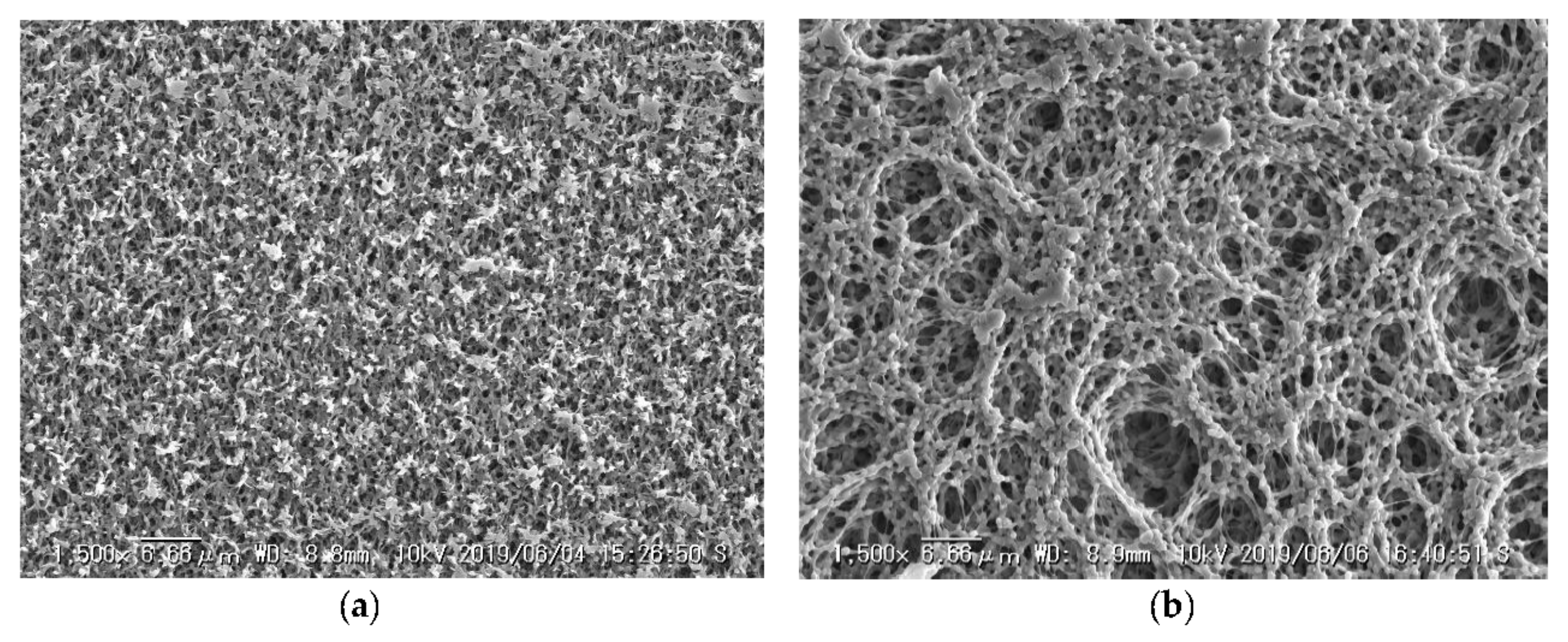
2.1. Selection of the Membrane Filter

Hydrophilic PVDF flat sheet membranes with a nominal pore size of 0.45 µm and a diameter of 47 mm (Merck Millipore HVLP04700, Darmstadt, Germany) were chosen for water filtration experiments and SEM imaging. Unlike 0.1 µm membranes (Merck Millipore VVLP04700, Darmstadt, Germany), 0.45 µm porous membranes presented a more open and thus heterogeneous structure on the surface, allowing us to acquire information on the underlying pores (Figure 1a,b). The complexity of the particle deposition within the pores, formation of particles clusters on the membrane surface, and the effect of small difference of feed water concentration on the homogeneity of particle distribution were observed on the 0.45 µm membranes, while all particles were retained on the membrane surface forming a cake layer on the 0.1 µm membranes. Thus, the 0.45 µm membranes were selected to observe intermediate stages of particle deposition on the membranes.

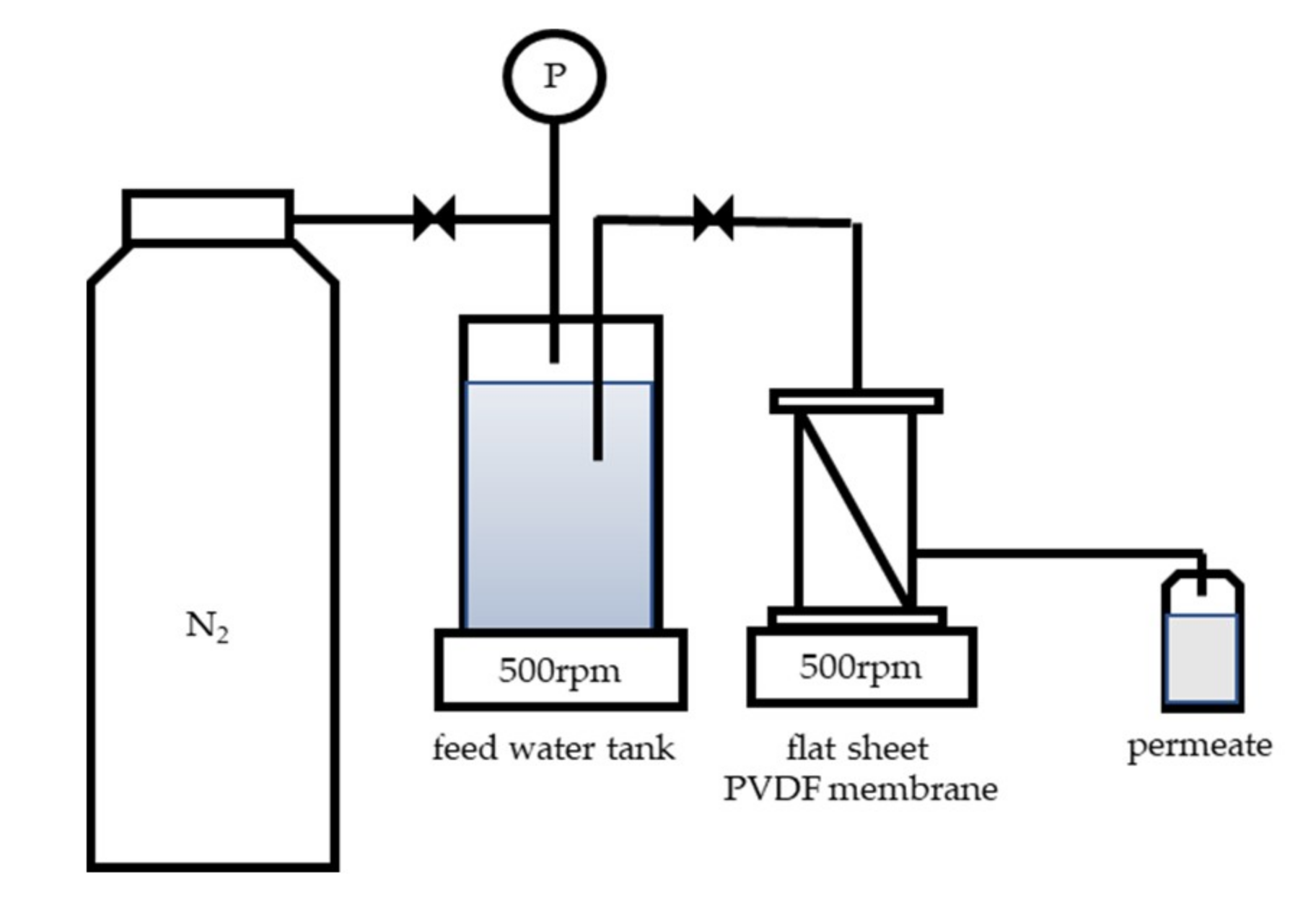
2.2. Filtration Experiments and Image Acquisition

To obtain the SEM images of particles deposited on the aforementioned PVDF flat sheet membranes, filtration experiments were carried out using the membrane filtration unit illustrated in Figure 2. We filtered 250 mL of Milli-Q water containing particles (1–9 mg/L, red fluorescent beads d = 0.5 µm, FluoroSpheres^TM carboxylate, F8812, Invitrogen by Thermo Fischer Scientific, Tokyo, Japan) for 2 min, through the membranes, at a constant pressure of 45 kPa. The feed water concentrations of 1–9 mg/L represent the range of suspended solids concentration of river water used for public water supply in Tokyo, Japan [24]. After the membrane filtration experiments, the membranes were taken out from the filtration unit and kept in a desiccator until their SEM images were taken by mode of secondary electron detection (1500×, 10 kV, Keyence VE-8800, WD: 8.8–8.9 mm, coating: Pt, high vacuum p = 10⁻³–10⁻⁴ Pa).

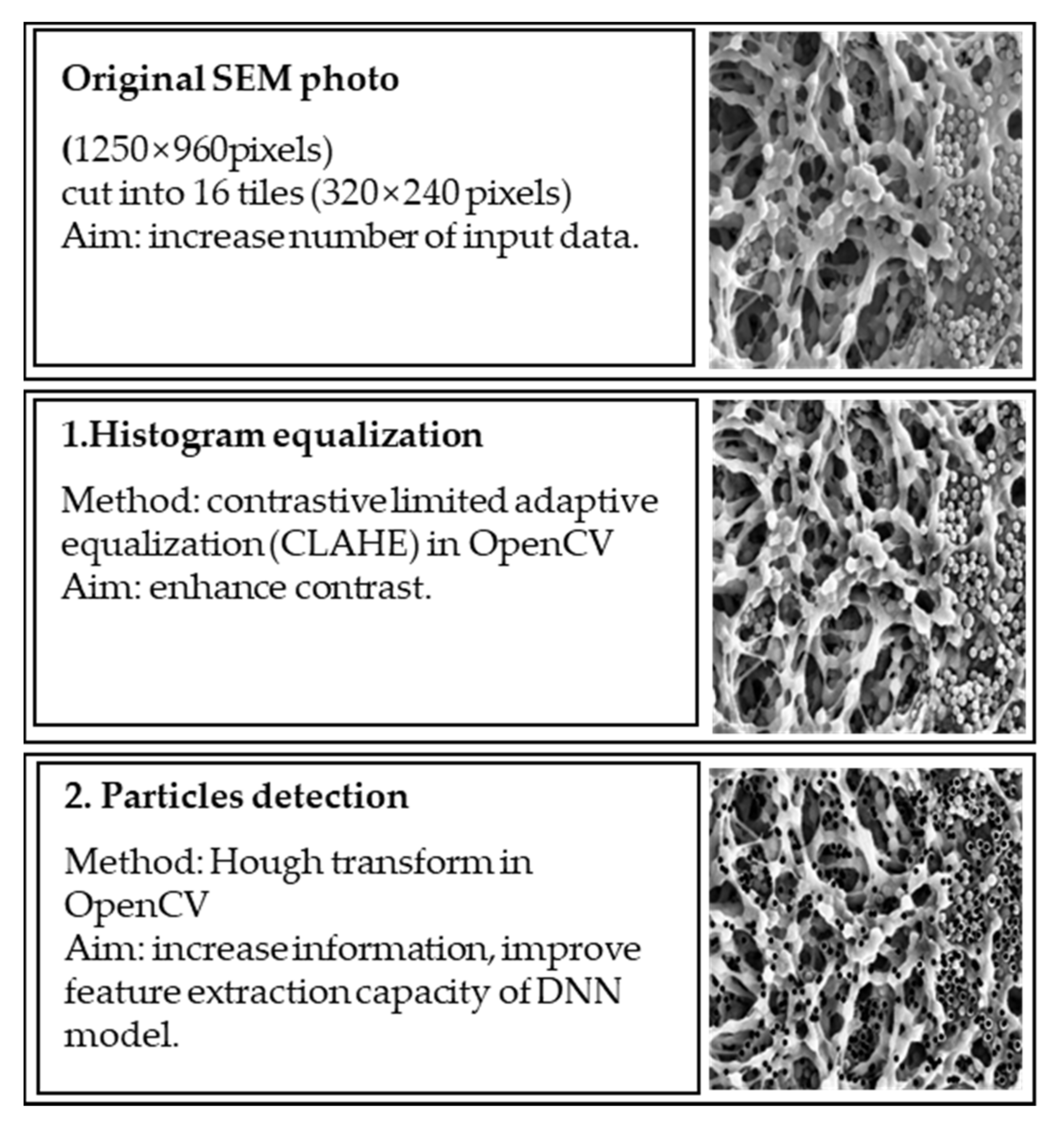
2.3. Image Preprocessing

The used flat sheet membranes after filtration, as well as the virgin membranes, were observed using the SEM, and 120 pictures (1280 × 960 pixels) were taken for each of the ten feed water concentrations, bringing the total number of images to 1200. To increase the number of input data, each image was split into 16 tiles (320 × 240 pixels), resulting in a total number of 19,200 images.

Image preprocessing was carried out to improve the feature extraction capacity and quality of information. SEM images used as input data were preprocessed by applying the Contrastive Limited Adaptive Equalization (CLAHE) algorithm of Open Source Computer Vision Library (OpenCV 4.0, Intel, Nižnij Novgorod, Russia), to obtain histogram equalization. By flattening the intensity pixel values, the contrast was enhanced, and the available image information was increased [25]. The OpenCV Hough transform algorithm was used to detect particles on the membrane surface. Particles were marked as black circles to enhance the model feature extraction capacity (Figure A1, Appendix A).

To initiate the training of the models, tiles (320 × 240 pixels) were reshaped (200 × 200) and uploaded as arrays of three dimensions, width, height, and channels, and were read as matrices of intensity values [26].

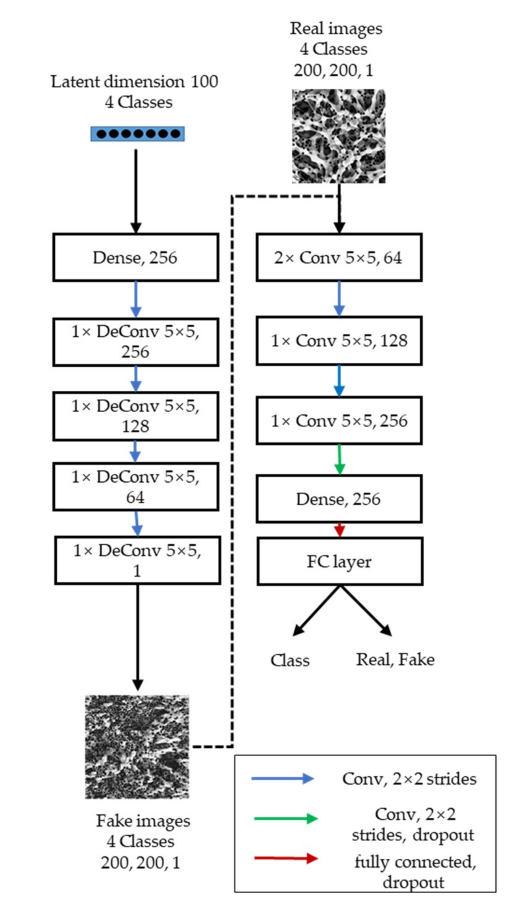
2.4. Particle Deposition Model Using ACGAN

To improve the stability of the generative adversarial network (GAN) training and the quality of generated images, conditioning the latent space by adding labels to the input data was found to be successful [27,28]. Auxiliary conditioning of ACGAN allows the generator to learn features faster and to output generated images belonging to different classes, satisfying the interest of describing particle deposition at different conditions of filtration. The four classes of membranes selected from the real input images for auxiliary conditioning were those of a virgin membrane and feed water concentrations of 2, 5, and 8 mg/L.

The ACGAN model architectures were developed using Keras, a high-level library written in Python (version 3.7.3), which enables working with the Tensorflow backend (Google brain, Mountain View, CA, USA).

The ACGAN model was structured according to the configurations shown in Figure 3 and reported in

Table A1. ACGAN Model configurations.

	Operation	Kernel 1	Stride 2	Feature Map 3	BN 4	Dropout 5	Activation Function 6
Discriminator	Convolution1	5 × 5	2 × 2	64	Yes		LeakyReLU
	Convolution2	5 × 5	2 × 2	64	Yes		LeakyReLU
	Convolution3	5 × 5	2 × 2	128	Yes		LeakyReLU
	Convolution4	5 × 5	2 × 2	256	Yes	0.5	LeakyReLU
	Dense			256, 1	Yes	0.5	Sigmoid (+Softmax)
Generator	Dense			256	Yes		LeakyReLU
	Deconvolutional1	5 × 5	2 × 2	256	Yes		LeakyReLU
	Deconvolutional2	5 × 5	2 × 2	128	Yes		LeakyReLU
	Deconvolutional3	5 × 5	2 × 2	64	Yes		LeakyReLU
	Deconvolutional4	5 × 5	2 × 2	1	Yes		tanh
	Discriminator input	200 × 200 × 1		Classes	4	Samples	7680
	Generator input	10 × 10 × 1		Output	200 × 200 × 1	Latent Space	100
	Batch size	30		Iterations	80,000	Optimizer	Adam lr = 0.0002

¹ Kernel: Array of weights of set pixels dimension that filters the input images, performing elementwise multiplication of own parameters and images pixel values to obtain a feature map. ² Stride: Parameter defining how the kernel slides on the input image. ³ Feature map: Output map of convolutional layers, composed of values for the specific features detected on the input image. ⁴ Batch Normalization: Regularizing technique to standardize activations of previous layers to zero mean and unit variance. ⁵ Dropout: Regularizing technique to drop out random sets of hidden units according to an indicated probability. ⁶ Activation function: Activation of summed weighted input from a node into the output. Can be linear (i.e., sigmoid, softmax, tanh) or non-linear (ReLU, Leaky ReLU) [26,34].

(Appendix A). The discriminator and generator were optimized for the specific type of images, through hyperparameter tuning, namely through adjustments of the layer depth, the kernel size, and the filter number, and by implementing regularization techniques, as suggested by Radford and Chintala [29]. The final model structure was chosen, based on the stability of the training process and on the quality of the output images.

2.5. Performance Evaluation

Currently there is a lack of a universally applied and valid way to evaluate the output of GANs in the literature [27]. Thus, in this study, among the proposed evaluation techniques, questionnaire based human validation and quantitative evaluation through particle counting were applied to the outputs of GANs. Human validation was carried out by setting up a google questionnaire form to evaluate the similarities between the real and generated images. The participants (n = 37) were required to determine if the displayed image (n = 20) was real or generated, after being given an example of both. The errors in predictions made by the interviewees are shown by use of a cumulative confusion matrix, where real images correspond to positive (1) and generated images to negative row (0). Thus, true positive signifies correctly predicted real images, false positive incorrectly predicted real images, true negative correctly predicted generated images and false negative incorrectly predicted generated images [30]. Particles on the generated images were counted both manually and automatically. Automatic counting on the generated images was performed through binarization of the generated images and contour detection (OpenCV) using pixel intensities and area as the thresholding values. Automatic counting on real images was performed through circles detection, using the Hough transform algorithm.

2.6. Density Clusters Identification

The density-based spatial clustering of application with noise (DBSCAN) algorithm was used to identify density clusters on real SEM images with deposited particles. DBSCAN is a machine learning data clustering algorithm that can group nearby points, based on distance measurements and a minimum number of samples [31]. Information on circle center coordinates were used as the input data and the minimum number of samples was set at 37, through trial and error.

2.7. Gini Index Equality Distribution and ANOVA

Gini index is a nonparametric statistical measure widely used in economics to assess the inequality in distribution of income and wealth between individuals in a population or between countries around the world [32]. Each of the 120 SEM images obtained at feed water concentrations of 1–9 mg/L were cut into 16 tiles and the tiles were ordered from the smallest to the largest particle counts; then the tiles of the same order were grouped so that each group had 120 tiles. Gini index and one-way ANOVA were used to analyze the differences of particle counts among those groups.

3. Results

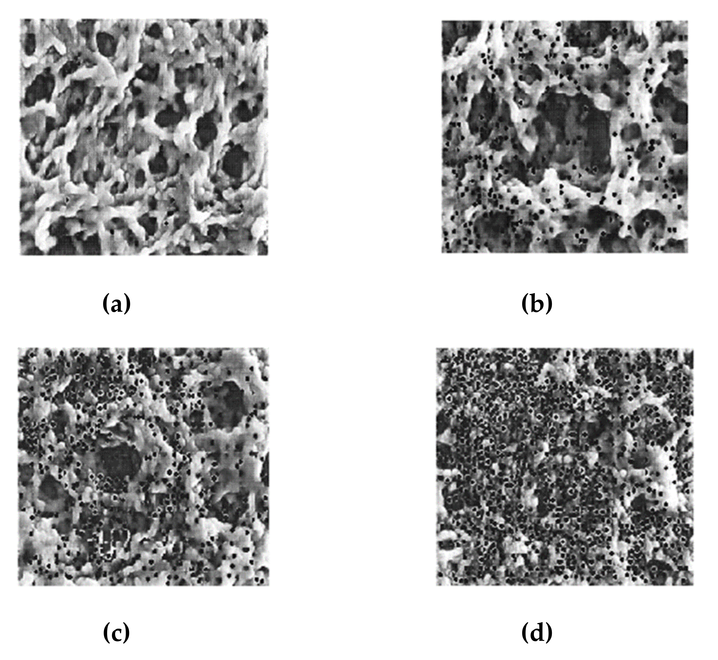
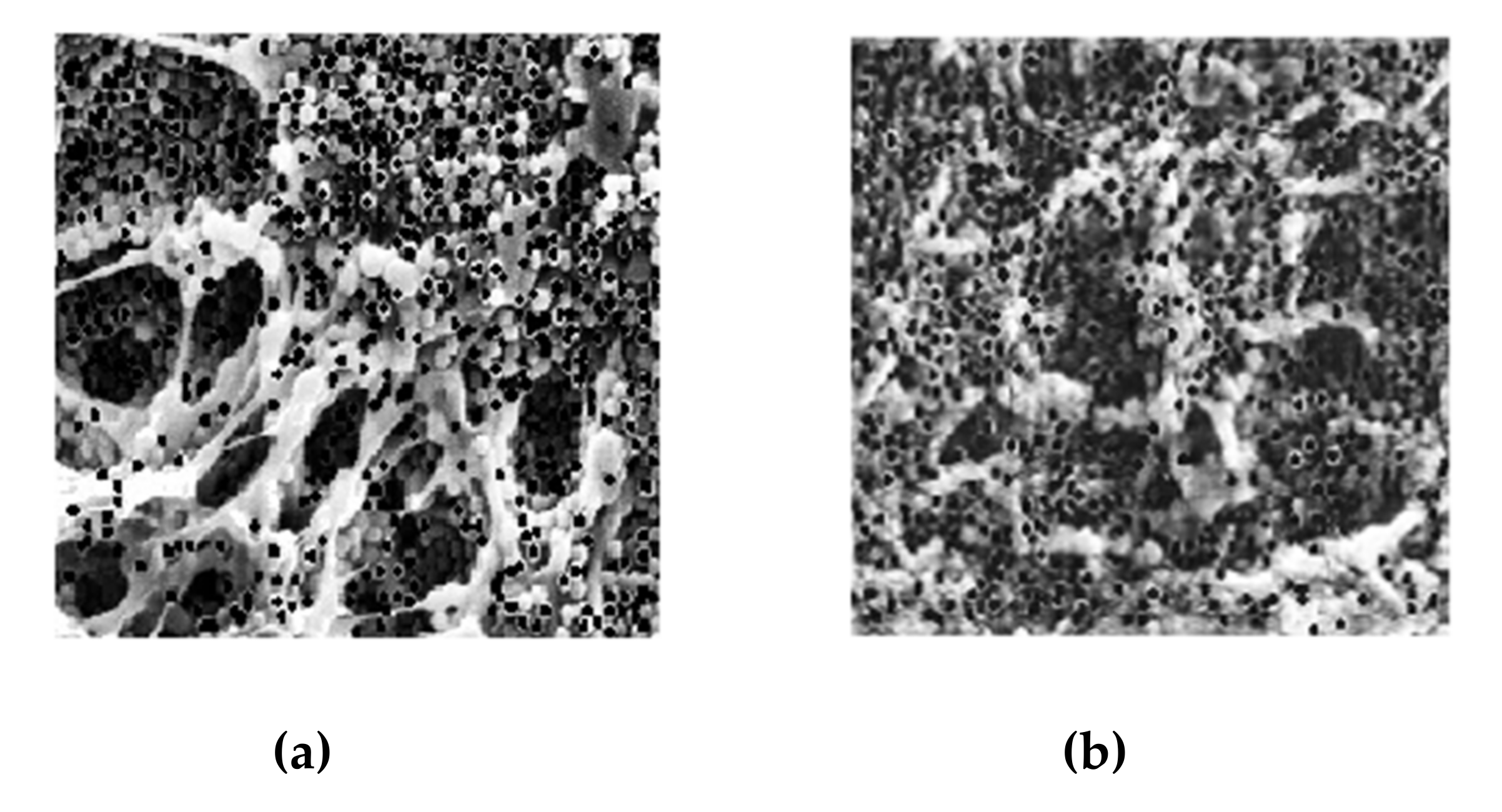
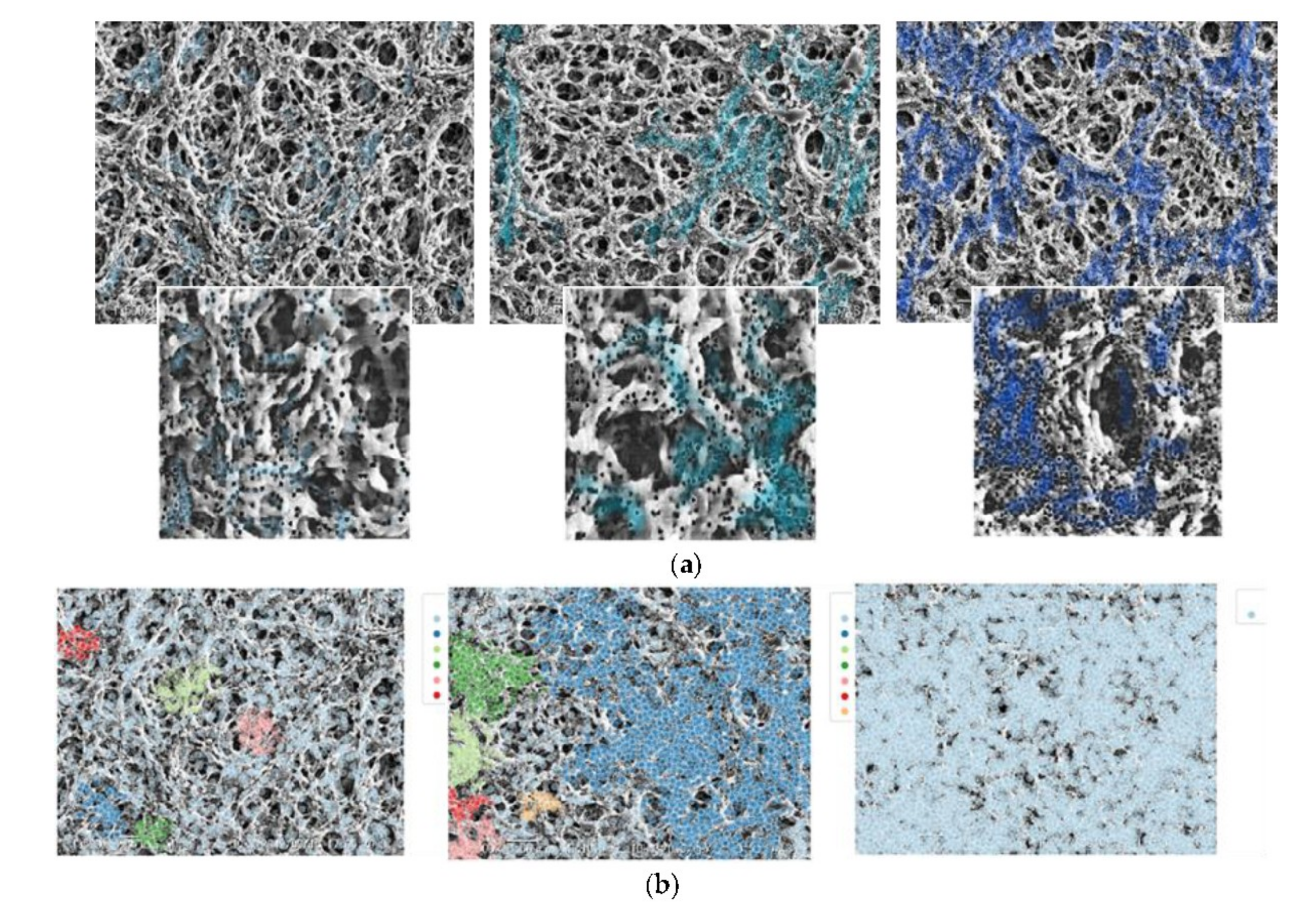
3.1. ACGAN Generated Images of PVDF Membranes with Deposited Particles

The ACGAN model was run for the maximum of 80,000 iterations, and the generated images were checked every 2560 iterations. The training was stable, and no convergence failure was observed, delivering images of impressive quality already, after 40,000 iterations (ca. 150 epochs). Figure 4 shows the plotted images for the four different classes (no particles, 2, 5, and 8 mg/L), after 74,240 iterations. The images represent the membrane structure quite accurately and the shapes, such as deep pores, visible as darker pixels, circular surface pores of bigger diameter, and crystal geometries as well as imperfection of the PVDF membrane structure, could be identified. In the images shown in Figure 4, the four classes of membranes are well represented by the increasing number of black dots, which indicate the deposited particles.

The development and hyperparameter tuning of the ACGAN model were, therefore, considered successful. Spotting particles as black dots in the preprocessing step resulted as an effective technique to enhance discrimination of those against pixels of the underlying and surrounding membrane structure.

3.2. Evaluation of ACGAN Generated Images of PVDF Membranes with Deposited Particles

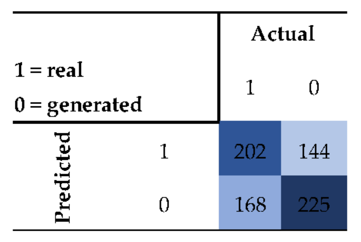
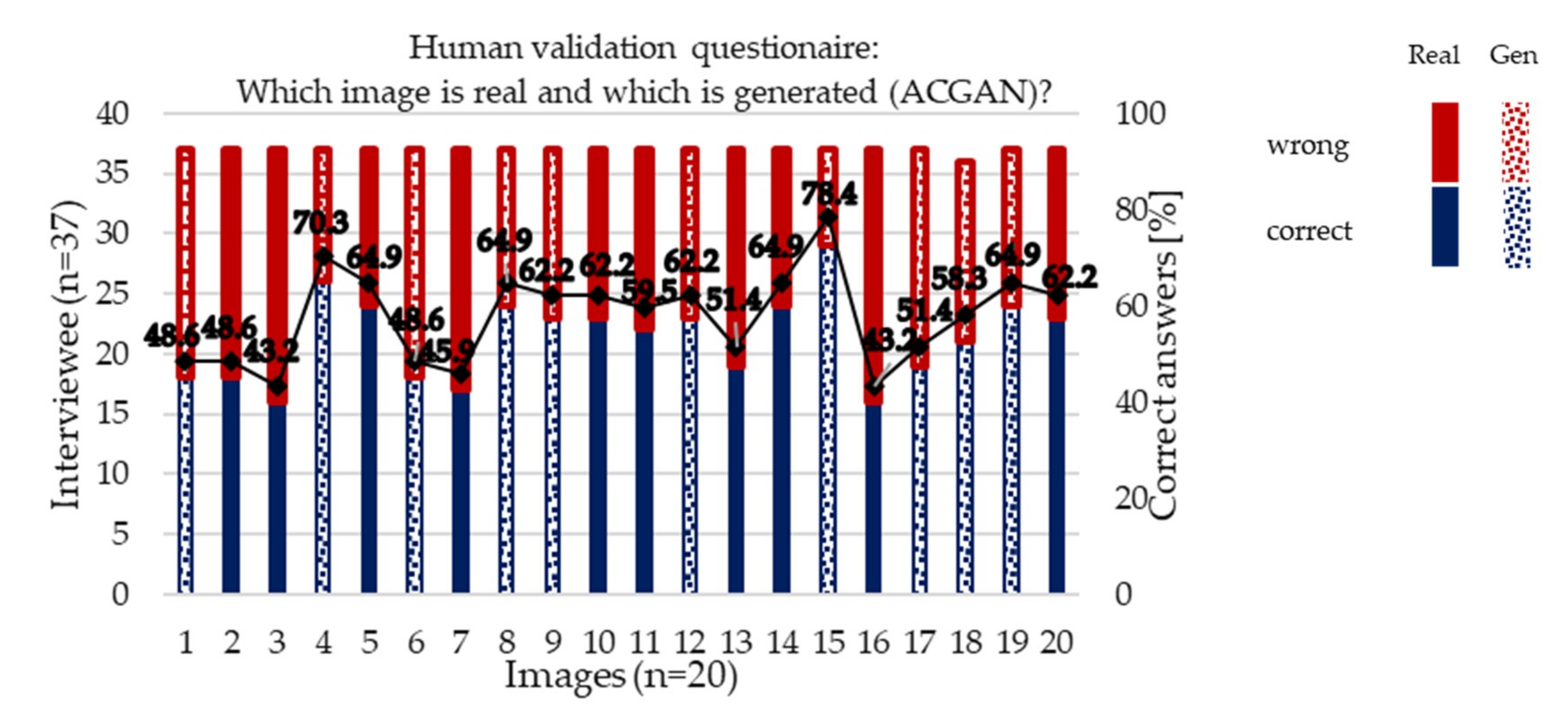
3.2.1. Human Validation

The results of human validation were summarized in a cumulative confusion matrix (Figure 5). The correct answers numbered 225 and 202 for the generated and real images, respectively, while the incorrect answers numbered 144 and 168, respectively. Hence, the overall accuracy was 57%, while the accuracies for the real and generated images were 54.6% and 61.0%, respectively, which indicated that the margin of accuracies between the real and generated images was small for human judgment. The results of human validation showed that their responses varied with the extent of randomness; hence, it was difficult for humans to distinguish between the real and generated images.

$$\mathit{Accuracy}=\frac{TP+TN}{TP+TN+FP+FN}=\frac{202+225}{202+225+144+168}=0.57$$

TP: True Positive, TN: True Negative, FP: False Positive, and FN: False Negative.

When looking at the replies to each image (Figure 6), for 30% of the images (two generated: ID 1 and 6; four real: ID 2, 3, 7, and 16), over 50% of the respondents identified the images incorrectly, whereas two images (generated ID 17; real ID 13) had only one vote difference, which indicated the same levels of difficulties of the real and generated images in finding the correct answers. Therefore, the high quality of these generated images was confirmed. Among those, specifically the real images (ID 3, 7, and 16), showed no visible characteristics that might have influenced the interviewees to incorrectly identify them as the generated images. On the other hand, the high accuracy of responses, 70.3% and 78.4% for generated images ID 4 and 15, respectively, might be due to the slightly lower quality of the displayed images, due to the mapping of random numbers drawn from the latent space (refer to Introduction). Thus, overall, the generated images successfully reconstructed the real images; however, there were a few generated images that needed to be excluded from further analysis.

When looking at the results of the human validation of real and generated images at 8 mg/L (Figure 7), the majority of the respondents wrongly identified two out of three images (Image ID 7, 15, and 16), meaning that humans were not able to correctly differentiate between the real and generated images at 8 mg/L as well. Thus, ACGAN was able to generate images of real 8 mg/L membranes. This is not evidence of the ACGAN model being capable of reproducing outlier images with smaller or bigger particle counts, as discussed later in the discussion section.

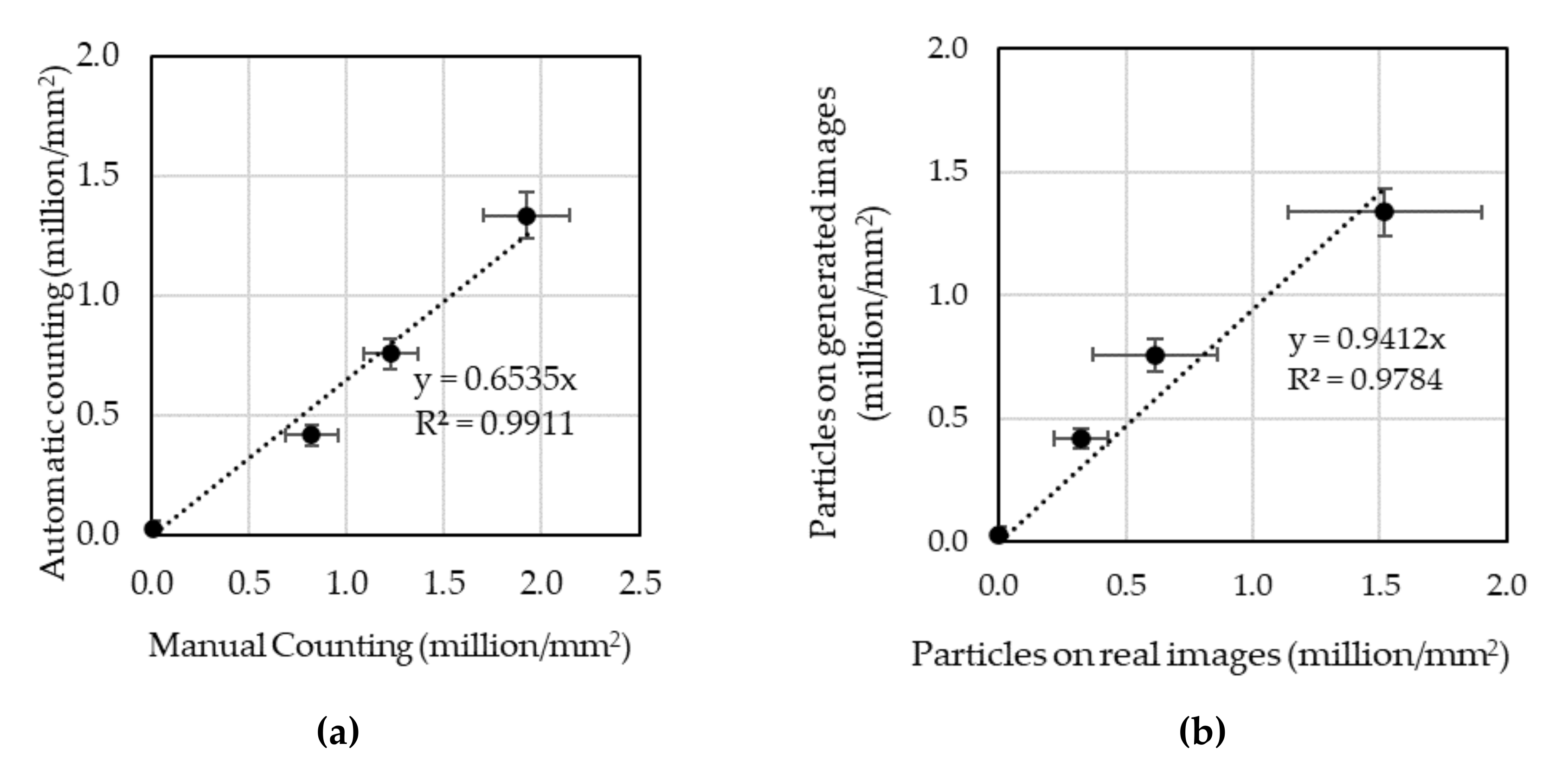
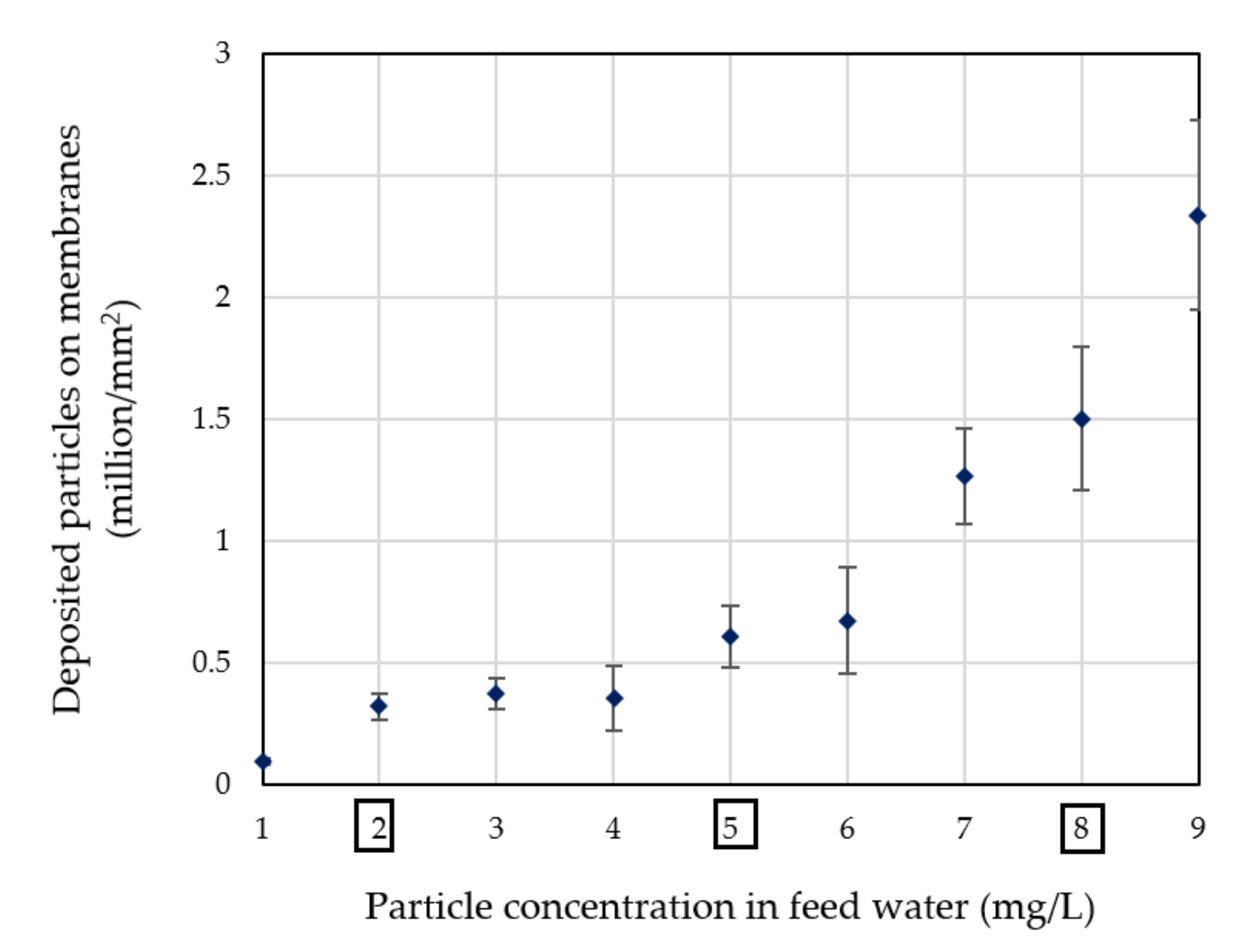
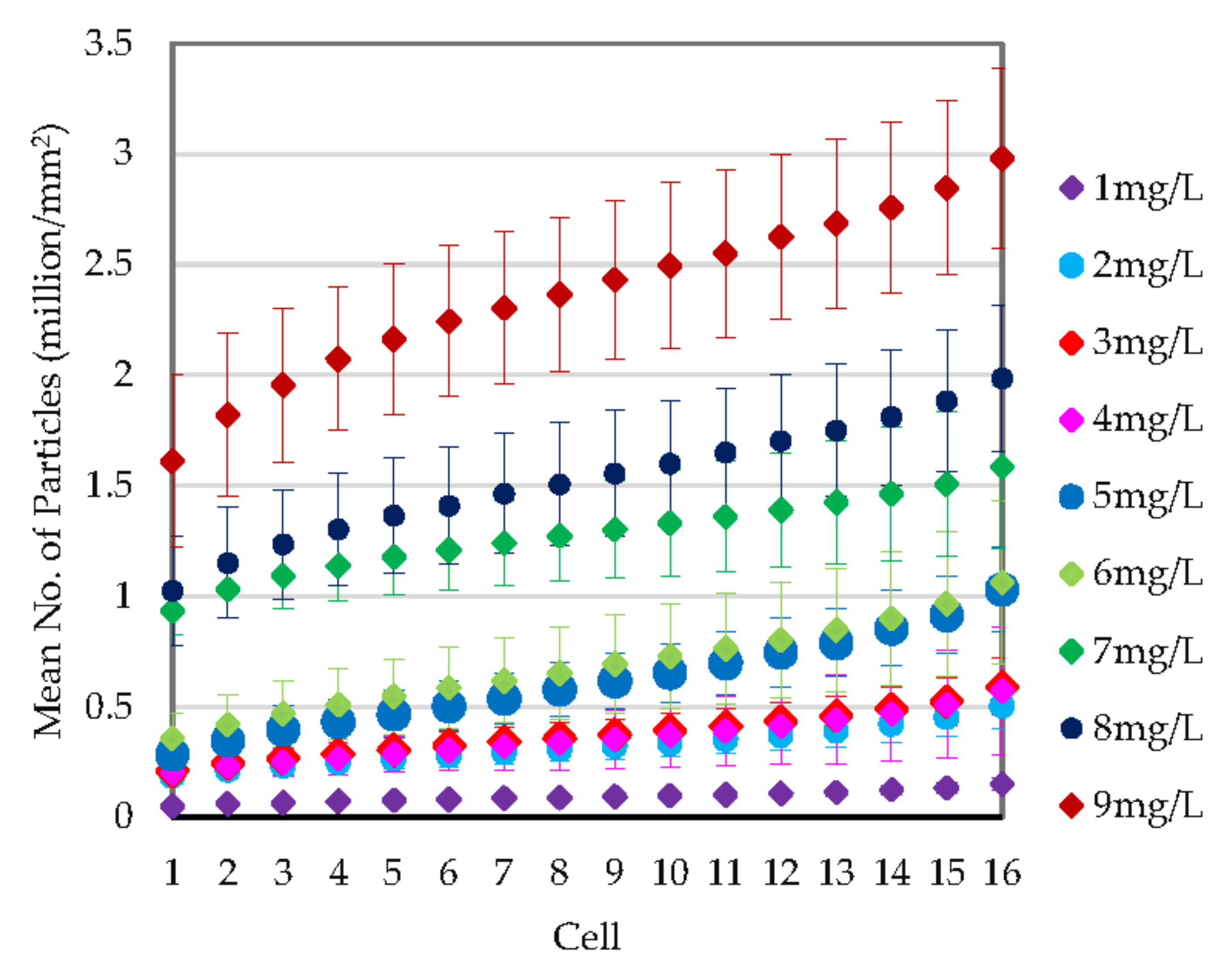
3.2.2. Quantitative Evaluation through Particle Counting

Particles on generated images were counted both manually and automatically (Figure 8a). The difference in the length of the bars, which represents the standard deviations, is due to the difference in the numbers of counted membranes, namely, automatic (n = 1920) vs. manual (n = 50), for each of the observed concentrations (0, 2, 5, and 8 mg/L). There was a linear relationship between manual and automatic particle counting; however, automatic particle counting was overall 34.6% less than those by manual particle counting. This result indicated that automatic counting had the tendency to underestimate the particle counts.

When comparing the mean number of particles on the real and generated images, several aspects could be noted (Figure 8b). At a particle concentration of 0 mg/L, the generated images showed a small number of particles, which might be interpreted as errors in the conditioning of the generator. The overall particle counts on generated images were 5.8% less than the particle counts on real images. The difference between the real and generated mean particle counts became greater when the feed water concentration was increased (up to a 185,597 mean particle count difference at 8 mg/L). Such an observation was partly explained by the application of two different methods for particle counting—circle detection through the Hough transform algorithm and contour detection based on pixel intensities and area thresholding for the real and generated images, respectively. The reason for applying different particle detection techniques is the inapplicability of the Hough transform for generated tiles, on which the particles did not appear as perfect circles, due to the lower quality of the images. The standard deviation of the particle counts on the real membranes increased with the feed water concentration, whereas the standard deviation of the generated images was significantly lower than those on the real images. Cake and multilayer deposition processes, which occur mainly at higher feed water concentrations, might explain the high variance in particle counts at higher feed water concentrations on real images, for which particle counting might be less precise due to the overlapping of circular elements. On the contrary, the standard deviation of the particle counts on the generated images were smaller than the real images, which might be because the ACGAN generated standard images rather than outlier images, far apart from the standard ones, while in the real membrane filtration there was an uneven distribution of particles deposited on the membranes. Thus, it could be said that the ACGAN model developed in this study was superb in reproducing particle deposition on the membranes filtered with low concentration particles in feed water, while at high feed water concentration, it tended to generate standard images of particles deposition, rather than outlier images of extremely high or low particle deposition.

4. Discussion

4.1. Particle Deposition Patterns on Real and Generated Images

Considering particle counts on full sized SEM images (n = 120 for each concentration), the following can be noted (Figure 9); at the feed water concentrations between 1 and 6 mg/L, the variance of particle counts on SEM images was low, and the retention did not increase linearly with increasing particle numbers in the feed water. However, at feed water concentrations greater than 6 mg/L, the number of retained particles increased significantly. The ratio of deposited particles on the membrane at 5 mg/L was the lowest (6.8%) in comparison to 2 mg/L (9.2%) and 8 mg/L (10.5%). We thus identified that there was a range of feed particle concentrations (approximately 5–6 mg/L), at which particle retention was smaller than at lower (1–4 mg/L) and higher concentrations (>6 mg/L).

Such a phenomenon was reported in stochastic-based modeling studies [15], mainly through the flux variation approach, rather than variations of feed particle concentrations. This observation could be further investigated through image analysis of the membranes deposited with particles at different initial feed water concentrations of 0, 2, 5, and 8 mg/L (Figure 10a,b). The highlighted areas on the top figures of Figure 10a (1280 × 960 pixels) indicate observed particle aggregates, whereas the bottom figures of Figure 10a show the corresponding ACGAN generated images (200 × 200 pixels). As the generated images represent only 1/16th of the real SEM size in Figure 10a, they are shown as slightly enlarged.

The density clusters identified on the SEM images of PVDF membranes by density-based spatial clustering of application with noise (DBSCAN) are shown in Figure 10b. The particle deposition patterns, which were reported in previous studies obtained through experimental and mathematical conventional approaches [5,8,12,15,30], were also recognized in these figures. Namely, at a low feed water concentration of 2 mg/L, the exclusion and attachment mechanisms seemed to be prevalent, with particles rejected by the same or smaller sized pores and particles attached on the membrane surfaces forming scattered small aggregates (Figure 10a,b far left).

The distribution of particle aggregates was similar for the real and generated images (Figure 10a); however, the differently colored images of particles identified by the DBSCAN showed more clearly that the particles penetrated deeply into the pores. The majority of the image shows homogenous and sparse distribution (light blue color in Figure 10b) that corresponded to sporadic attachments of particles, both in deep pores, membrane edges, and crystal structures, while there were several small aggregates, mostly on membrane surfaces, which suggested the prevalence of particle–membrane interactions over particle–particle interactions (Figure 10b). This kind of attachment behavior was identified as the first step of the fouling process in the multi-mechanism fouling model proposed by Griffiths et al. [8].

The density of the attached particles on the membrane surfaces increased further at 5 mg/L of feed water on the real and generated images (Figure 10a middle), but they could not show the particles deposited inside the pores. In contrast, the DBSCAN images successfully showed particles both deep inside and on the surface of the membrane pores. In addition, the particles were mostly found in aggregates, seemingly depositing on the initially blocked smaller pores or again surrounding larger membranes structures (Figure 10a). DBSCAN analysis showed the highest and widest distribution in cluster numbers, confirming the tendency of particles to assemble, as the particle–particle interactions became stronger (Figure 10b).

As Park et al. [9] showed through their analysis of fouling formation on RO/NF membranes, the influence of membrane properties on the fouling processes decreased as the membrane surface became saturated with foulants. The similar patterns of particle deposition on the real and generated images (Figure 10a) indicated that the particles first attached and aggregated on membrane surfaces near small pores, which led to the clogging of small pores. Then, the share in the flux through larger pores increased as they remained free of particles, as can be seen on the SEM and the generated images, consequently increasing the probabilities of particles passing through the membrane. This process was clearly seen at 5 mg/L—the small pores were blocked faster than at 2 mg/L, thus, enhancing the flux through the larger pores, which resulted in lower particle retention rates. The experimental results by Beuscher [15] for the filtration of a 50 nm beads suspension through membranes of different pore sizes (0.02–0.04 µm) reported an overall decrease in the retention efficiency, which could not be explained if size exclusion was the only phenomenon at play. Thus, it was estimated that the water flux was diverted to large pores, due to the clogging of small pores.

At 8 mg/L, the particles deposited on the membrane formed a large aggregate, as observed by DBSCAN, but the real SEM and generated images showed only the surface deposition of particles. These results indicated that the DBSCAN is a useful tool to identify the total numbers of particles attached or deposited on the membrane, while the SEM images were useful for the identification of particles deposited on surfaces. Thus, a combination of SEM or ACGAN images with DBSCAN analysis is a useful method to identify particles deposited on both membrane surfaces and inside large pores.

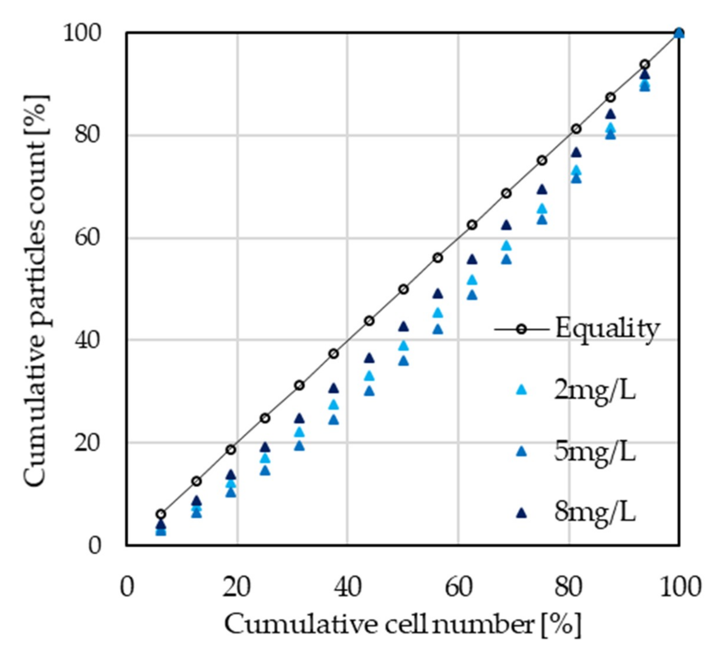
4.2. Particle Distribution Analysis through Gini Index Calculation

As shown in Figure 7b, the particle counts on the real membranes had a higher variance than the ACGAN generated membranes. To measure the deviation from the equal distribution of particles deposited on the membranes, a total of 120 SEM images were cut into 16 cells and the particles on each of the 16 cells were counted. Then, the 16 cells of each of the 120 SEM images were sorted from the smallest to the largest. The averages and standard deviations were calculated for each of the 16 cells for 120 images (Figure 11). At each feed water concentration, a sigmoidal trend could be seen from cell 1 to cell 16, namely from the lowest to the highest number of retained particles. For all feed water concentrations, except for 3 mg/L (p = 0.07), there was a statistically significant difference in the number of deposited particles counted on the 16 cells (ANOVA, p < 0.05). If the membrane was produced completely equally on all portions of the membrane, the number of particle depositions should be equal among all 16 cells. This indicated that the ratio between the largest particle number of a cell (cell number 16), over the smallest (cell number 1) could be an indicator of the variance in the retention efficiency of the membrane at each feed water concentration. This ratio was the largest at 3.63 at 5 mg/L, compared to other feed water concentrations. This conclusion agreed with the observations previously carried out (Section 4.1) and those shown in Figure 10.

The cumulative particle counts on the 16 cells for different feed water concentrations were further plotted to draw the Lorenz Curves and thereby to obtain the Gini Index equality coefficient (Figure 12). For all feed water concentrations, the Gini Index did not surpass 0.20, indicating only a slight unevenness in the particle distribution on the membrane surface. It could be noted, though, that the Gini Index increased from 1 mg/L (GI = 0.160), reaching its maximum at 5 mg/L (GI = 0.193), and then decreased to its minimum at 9 mg/L (GI = 0.091). The Lorenz curves for the SEM images at 2, 5, and 8 mg/L (Figure 12) could be related to the deposition patterns previously described and observed for the real and generated SEM images, as well as to the density clusters identified using the DBSCAN algorithm (Figure 10). At 2 mg/L (G = 0.152), higher equality in the distribution corresponded to random attachments of particles on membrane materials and in deep pores. At 5 mg/L, the inequality in distribution was the highest (G = 0.193) and so was the tendency of particles to cluster, giving in to particle–particle interactions. As the pores were blocked and a cake layer started forming on the surface of the membrane, at 8 mg/L, the distribution of particles drew near the line of equality (G = 0.10) and was homogenous.

Observing the intermediate steps leading to internal fouling is a very helpful indicator of the process of particle deposition and should be accounted for, with the aim of optimizing the porous filtration processes, and cleaning practices and schedules. Special account should be taken regarding particles, as the smaller particles were already reported as the main contributor of membrane fouling and flux decline because they shorten the initial internal pore blocking phase [33].

5. Conclusions

An auxiliary classifier generative adversarial network (ACGAN) model was developed to reproduce membrane fouling by particle deposition, using SEM photos of PVDF 0.45 µm porous membranes. We verified—by both human judgment and particle counting on the real and generated images—that the ACGAN model developed in this study could regenerate the images of particle-deposited membranes. There was a limitation, however, especially at a high particle concentration, that the ACGAN model tended to produce standard membrane images with smaller standard deviations rather than those of the real SEM images.

Furthermore, the particle deposition patterns of the real SEM and generated images proved that these images had the same patterns of the particle deposition processes, which indicated the effectiveness of ACGAN-generated images to simulate the particle deposition processes on filtration membranes. The particle deposition and formation of aggregate on the membranes were compared to the particle deposition and aggregation analysis through density-based spatial clustering of application with noise (DBSCAN). It was found that, while the SEM and generated images were useful to identify the particles deposited on the membrane surface, DBSCAN was able to identify the particles deposited on both the surface and inside the pores of the membrane images. Thus, a combined use of these two methods would make it possible to work with both membrane surfaces and inside pores.

To investigate the deviance of particle distribution on the real, rather than generated, membranes, the membrane images were cut into 16 cells, and the number of particles were counted for each of those cells. As a result, the inequality of particle distribution was the highest at the median feed water concentration, with the clustering of particles on membrane surfaces. At lower and higher feed concentrations, the particle distribution was more even, which might be linked to the random initial attachment of the particles and homogenous cake layer formation, respectively. These results provided insight into the different particle retention rates at various feed water concentrations.

The ACGAN model developed in this research was useful for feature extraction of the fouled membranes and provided an alternative modeling method of membrane fouling in water filtration that could represent the actual porous membrane structure, and thereby, overcome the constraints of over-simplification of the real membrane structures in the previous studies. The adaptability of the deep neural network (DNN) models including ACGAN to model membranes of any structure is a further strength, while the conventional physical models must be developed for each specific type of membranes. Although the provided ACGAN model is readily available for data augmentation applications, its potential has yet to be explored in further research, which should consider the generations of images for which real SEM images are not available, such as at varied filtration conditions, without the need of carrying out experiments. This would allow, with a minimum input of real SEM images, actual sequence predictions of particle deposition. The satisfying quality and diversity of generated images, as well as the capability to reproduce particle deposition patterns observed on real SEM images, confirms the future need to explore diverse DNNs in the field of membrane science, to improve our understanding of membrane fouling processes.

References

1. Alspach, B.; Adham, S.; Cooke, T.; Delphos, P.; Garcia-Aleman, J.; Jacangelo, J.; Karimi, A.; Pressman, J.; Schaefer, J.; Sethi, S. Microfiltration and ultrafiltration membranes for drinking water. J. Am. Water Work. Assoc. 2008, 100, 84–97. [Google Scholar]
2. Warsinger, D.M.; Chakraborty, S.; Tow, E.W.; Plumlee, M.H.; Bellona, C.; Loutatidou, S.; Karimi, L.; Mikelonis, A.M.; Archilli, A.; Ghassemi, A.; et al. A review of polymeric membranes and processes for potable water reuse. Prog. Polym. Sci. 2018, 81, 209–237. [Google Scholar] [CrossRef] [PubMed]
3. Van der Bruggen, B. Microfiltration, ultrafiltration, nanofiltration, reverse osmosis, and forward osmosis. Fundam. Modeling Membr. Syst. 2018, 25–70. [Google Scholar]
4. Singh, R.; Hoffmann, E.J.; Judd, S. Membrane Technology and Engineering for Water Purification; Membranes Technology ebook Collection; Elsevier: Amsterdam, Netherlands, 2008. [Google Scholar]
5. Krupp, A.U.; Griffiths, M.; Please, C.P. Stochastic modelling of membrane filtration. Proc. R. Soc. 2017, 473, 20160948. [Google Scholar] [CrossRef] [PubMed] [Green Version]
6. Guo, W.; Ngo, H.-H.; Li, J. A mini review on membrane fouling. Bioresour. Technol. 2012, 122, 27–34. [Google Scholar] [CrossRef] [PubMed]
7. Lohaus, J.; Perez, Y.M.; Wessling, M. What are the microscopic events of colloidal membrane fouling? J. Membr. Sci. 2018, 553, 90–98. [Google Scholar] [CrossRef] [Green Version]
8. Griffiths, I.M.; Kumar, A.; Stewart, P.S. A combined network model for membrane fouling. J. Colloid Interface Sci. 2014, 432, 10–18. [Google Scholar] [CrossRef] [Green Version]
9. Park, S.; Baek, S.-S.; Pyo, J.C.; Pachepsky, Y.; Park, J.; Cho, K.H. Deep neural networks for modeling fouling growth and flux decline during NF/RO membrane filtration. J. Membr. Sci. 2019, 587, 117164. [Google Scholar] [CrossRef]
10. Shetty, G.R.; Chellam, S. Predicting membrane fouling during municipal drinking water nanofiltration using artificial neural networks. J. Membr. Sci. 2003, 217, 69–86. [Google Scholar] [CrossRef]
11. Ando, T.; Akamatsu, K.; Fujita, M.; Nakao, S. Direct Simulation Model of Concentrated Particulate Flow in Pressure-Driven Dead-End Microfiltration. J. Chem. Eng. Jpn. 2010, 43, 815–828. [Google Scholar] [CrossRef] [Green Version]
12. Mino, Y.; Sakai, S.; Matsuyama, H. Simulations of particulate flow passing through membrane pore under dead-end and constant pressure filtration condition. Chem. Eng. Sci. 2018, 190, 68–76. [Google Scholar] [CrossRef]
13. Abdoli, S.M.; Shafiei, S.; Raoof, A.; Ebadi, A.; Jafarzadeh, Y.; Aslannejad, H. Water Flux Reduction in Microfiltration Membranes: A Pore Network Study. Chem. Eng. Technol. 2018, 41, 1566–1576. [Google Scholar] [CrossRef]
14. Xiong, Q.; Baychev, T.G.; Jivkov, A.P. Review of pore network modeling of porous media: Experimental characterizations, network constructions and applications to reactive transport. J. Contam. Hydrol. 2016, 192, 101–117. [Google Scholar] [CrossRef] [PubMed]
15. Beuscher, U. Modeling Sieving Filtration Using Multiple Layers of Parallel Pores. Chem. Eng. Technol. 2010, 33, 1377–1381. [Google Scholar] [CrossRef]
16. Bowen, R.W.; Joes, M.G.; Welfoot, J.S.; Yousef, H.N.S. Predicting salt rejections at nanofiltration membranes using artificial neural networks. Desalination 2000, 129, 147–162. [Google Scholar] [CrossRef]
17. Baeldung. Genetic Algorithms vs Neural Networks. Baeldung. 2020. Available online: https://www.baeldung.com/cs/genetic-algorithms-vs-neural-networks (accessed on 30 June 2020).
18. Hua, F.; Fang, Z.; Qiu, T. Modeling Ethylene Cracking Process by Learning Convolutional Neural Network. Comput. Aided Chem. Eng. 2000, 44, 841–846. [Google Scholar]
19. Liu, Q.-F.; Kim, S.-H. Evaluation of membrane fouling models based on bench-scale experiments: A comparison between constant flowrate blocking laws and artificial neural network (ANNs) model. J. Membr. Sci. 2008, 310, 393–401. [Google Scholar] [CrossRef]
20. Kowalik-Klimczak, A.; Bednarska, A.; Gradkowski, M. Scanning Electron Microscopy (SEM) in the Analysis of the Structure of Polymeric Nanofiltration Membranes. Probl. Eksploat.-Maint. 2016, 100, 119–128. [Google Scholar]
21. De Rover, E.W.F.; Huisman, I.H. Microscopy as a tool for analysis of membrane failure and fouling. Desalination 2006, 207, 35–44. [Google Scholar] [CrossRef]
22. Standfort, V.; Yan, K.; Pickhardt, P.J.; Summers, R.M. Data augmentation using generative adversarial networks (CycleGAN) to improve generalizability in CT segmentation tasks. Sci. Rep. 2019, 9, 16884. [Google Scholar] [CrossRef]
23. Nicholson, C. A Beginner’s Guide to Generative Adversial Networks (GANs). 2019. Available online: https://skymind.ai/wiki/generative-adversarial-network-gan (accessed on 14 October 2019).
24. Tokyo Metropolitan Waterworks, Water Quality Report. Available online: https://www.waterworks.metro.tokyo.jp/data/suigen/kekka30/j003-4.pdf (accessed on 30 June 2020).
25. Bovik, A.C. Basic Gray Level Image Processing. In The Essential Guide to Image Processing; Academic Press: Cambridge, MA, USA, 2009. [Google Scholar]
26. Deshpande, A. A Beginner’s Guide to Understand Convolutional Neural Networks. 2016. Available online: https://adeshpande3.github.io/adeshpande3.github.io/A-Beginner’s-Guide-To-Understanding-Convolutional-Neural-Networks/ (accessed on 26 June 2019).
27. Brownlee, J. Generative Adversarial Networks with Python: Deep Learning Generative Models for Image Synthesis and Image Translation; Machine Learning Mastery: Vermont, VIC, Australia, 2019. [Google Scholar]
28. Odena, A.; Olah, C.; Shlens, J. Conditional Image Synthesis with Auxiliary Classifiers GANs. In Proceedings of the 34th International Conference on Machine Learning, Sydney, Australia, 6–11 August 2017. [Google Scholar]
29. Radford, A.; Chintala, S. Unsupervised Learning with Deep Convolutional Generative Adversial Networks. Machine Learning; Cornell University: Ithaca, NY, USA, 2017. [Google Scholar]
30. Brownlee, J. How to Code Algorithms from Scratch with Python. In What Is a Confusion Matrix in Machine Learning; Machine Learning Mastery: Vermont, VIC, Australia, 2019. [Google Scholar]
31. Salton do Prado, K. How DBSCAN Works and Why Should We Use it. 2017. Available online: https://towardsdatascience.com/how-dbscan-works-and-why-should-i-use-it-443b4a191c80 (accessed on 20 April 2020).
32. Wright Muelas, M.; Mughal, F.; O’Hagan, S.; Day, P.J.; Kell, D.B. The role and robustness of the Gini coefficient as an unbiased tool for the selection of Gini genes for normalizing expression profiling data. Sci. Rep. 2019, 9, 1–21. [Google Scholar] [CrossRef] [PubMed]
33. Lim, A.L.; Bai, R. Membrane fouling and cleaning in microfiltration of activated sludge wastewater. J. Membr. Sci. 2003, 216, 279–290. [Google Scholar] [CrossRef]
34. Raschka, S.; Mirjalili, V. Python Machine Learning, 2nd ed.; Packt Publishing Ltd.: Birmingham, UK, 2017. [Google Scholar]
Figure 1. Scanning electron microscope (SEM) photos of virgin polyvinyl difluoride (PVDF) flat sheet membranes (1280 × 960 pixels, 1500×, 10 kV, VE-8800, Keyence, Osaka, Japan); (a) pore size = 0.1 µm, and (b) pore size = 0.45 µm.
Water 12 02225 g001
Figure 2. Experimental setup for the filtration of feed water particles through a flat sheet membrane.
Water 12 02225 g002
Figure 3. Auxiliary classifier generative adversarial networks (ACGAN) model structure configurations.
Water 12 02225 g003
Figure 4. ACGAN generated images of the PVDF membrane structure and particles for four different particle concentrations in feed water (a) 0, (b) 2, (c) 5, and (d) 8 mg/L (200 × 200 pixels).
Water 12 02225 g004
Figure 5. The cumulative confusion matrix of all responses (n = 739) for the discrimination of real and generated ACGAN images questionnaire.
Water 12 02225 g005
Figure 6. Interviewee (n = 37) responses to the discrimination of real and generated ACGAN images questionnaire.
Water 12 02225 g006
Figure 7. Examples of (a) real and (b) generated SEM images at 8 mg/L feed water concentration.
Water 12 02225 g007
Figure 8. Particle counts on membranes at four different initial concentrations (0, 2, 5, and 8 mg/L, n = 1920 for each concentration): (a) comparison between the manual and automatic counts on generated images, and (b) comparison between the particle counts on the real and generated images by automatic counting. The bars indicate the standard deviations.
Water 12 02225 g008
Figure 9. Mean number of particles for 1–9 mg/L feed water particles concentrations detected per mm2 membrane area on equalized SEM photos of PVDF flat sheet membranes (n = 120 for each particle concentration, 1280 × 960 pixels, 1500×, 10 kV, Keyence VE-8800).
Water 12 02225 g009
Figure 10. The real and generated images of PVDF flat sheet membranes at feed water concentrations of 2, 5, and 8 mg/L (from left to right)—(a) highlighted patterns of particle depositions on real (top: 1280 × 960 pixels) and generated images (bottom: 200 × 200 pixels), and (b) particle clusters on real images identified by density-based spatial clustering of applications with noise (DBSCAN).
Water 12 02225 g010
Figure 11. Particle distribution on 16 cells of SEM images, ordered from the minimum to the maximum particle counts. Error bars indicate standard deviation.
Water 12 02225 g011
Figure 12. The Lorenz curve for the cumulative particle counts to cumulative cell numbers for SEM images. Feed water concentration—2, 5, and 8 mg/L.
Water 12 02225 g012