Abstract
Long-term trends in reference evapotranspiration (ETref) and its controlling factors are critical pieces of information in understanding how agricultural water requirements and water resources respond to a variable and changing climate. In this study, ETref, along with climate variables that directly and indirectly impact it, such as air temperature (T), incoming solar radiation (Rs), wind speed (u), relative humidity (RH), and precipitation (P), are discussed. All variables are analyzed for four weather stations located in irrigated agricultural regions of inter-mountain Wyoming: Pinedale, Torrington, Powell, and Worland. Non-parametric Mann−Kendall (MK) trend test and Theil–Sen’s slope estimator were used to determine the statistical significance of positive or negative trends in climate variables and ETref. Three non-parametric methods—(i) Pettitt Test (PT), (ii) Alexandersson’s Standard Normal Homogeneity Test (SNHT), and (iii) Buishand’s Range Test (BRT)—were used to check the data homogeneity and to detect any significant Trend Change Point (TCP) in the measured data time-series. For the data influenced by serial correlation, a modified version of the MK test (pre-whitening) were applied. Over the study duration, a statistically significant positive trend in maximum, minimum, and average annual temperature (Tmax, Tmin, and Tavg, respectively) was observed at all stations, except for Torrington in the southeast part of Wyoming, where these temperature measures had negative trends. The study indicated that the recent warming trends are much more pronounced than during the 1930s Dust Bowl Era. For all the stations, no TCPs were observed for P; however, significant changes in trends were observed for Tmax and Tmin on both annual and seasonal timescales. Both grass and alfalfa reference evapotranspiration (ETo and ETr) had statistically significant positive trends in at least one season (in particular, the spring months of March, April, and May (MAM) or summer months of June, July, and August (JJA) at all stations, except the station located in southeast Wyoming (Torrington) where no statistically significant positive trends were observed. Torrington instead experienced statistically significant negative trends in ETo and ETr, particularly in the fall months of SON and winter months of DJF. Over the period-of-record, an overall change of +26, +31, −48, and +34 mm in ETo and +28, +40, −80, and +39 mm in ETr was observed at Pinedale, Powell, Torrington, and Worland, respectively. Our analysis indicated that both ETo (−3.4 mm year−1) and ETr (−5.3 mm year−1) are decreasing at a much faster rate in recent years at Torrington compared to other stations. Relationships between climate variables and ETo and ETr on an annual time-step reveal that ETo and ETr were significantly and positively correlated to Tavg, Tmax, Rs, Rn, and VPD, as well as significantly and negatively correlated to RH.
1. Introduction
Understanding long-term climatic trends at regional and local scales can help alleviate potential negative effects on agro-ecosystem productivity and aid in the development of effective climate change mitigation and adaptation strategies [1]. The influence of climate change/variability on agricultural production and water resources depends on the local magnitude and timing of variability, as well as mitigation and adaption practices undertaken [2,3]. According to the Intergovernmental Panel on Climate Change (IPCC) Fifth Assessment Report, National Aeronautics and Space Administration (NASA), and National Oceanic and Atmospheric Administration (NOAA), in the span of last hundred and thirty-six years, seventeen of the eighteen warmest years occurred after 2001. On a global scale, the years 2016, 2019, and 2015 ranked as the warmest, second warmest, and third-warmest for the period-of-record, with average global temperature anomalies of +0.99 °C, +0.95 °C, and +0.86 °C, respectively, compared to the 1951−1980 average. The global surface temperature is projected to increase by an additional 0.4 °C by 2025 [4]. This shift could have serious impacts on agricultural productivity and regional freshwater resources.
In general, projections of local and regional temperature changes are uncertain, particularly when inferred from general circulation models (GCMs), which typically have a spatial resolution of 1° or 2°, which is far coarser than the scale at which regional and local-level processes and decisions occur [5]. In situ monitoring of locally observed data and trends is thus essential for documenting changes in climatic conditions at a scale relevant to agriculture. In addition, with the change in land surface/air temperature measures, meteorological variables which are directly and indirectly related to temperature (e.g., vapor pressure deficit, evaporation from the surface, transpiration from vegetation surfaces, and crop evapotranspiration (ETc)) can be affected significantly. Changes in atmospheric temperature also affect precipitation, relative humidity, wind speed, and direction through an influence on regional atmospheric circulation patterns. Among these variables, ETc is one of the most important and largest components of the hydrological cycle. ETc represents a direct response of water losses from agricultural fields and is a powerful indicator of crop water productivity [6]. Accurate estimation of ETc is also important for irrigation management, quantification of water supply and demand, water allocations, and other hydrological processes. In general, direct measurement of ETc is generally difficult and expensive, requiring advanced instrumentation such as Eddy Covariance Systems, Bowen Ratio Energy Balance Systems, or Lysimeters. Therefore, in many cases, ETc is estimated from reference (potential) evapotranspiration (ETref) adjusted with crop coefficients (Kc) using the Food and Agricultural Organisation (FAO) Irrigation and Drainage paper number 56 approach. The crop coefficient is an integrated factor that incorporates crop canopy characteristics, irrigation method, management practices, and soil−water conditions [7]. On the other hand, ETref is an integrated climatic parameter that measures evaporative demand of the atmosphere. Many studies found good agreement between Penman−Monteith-estimated (potential) ETref with Lysimeter and Eddy covariance-measured ETref on grass surface [8]. In the semi-arid condition of Spain, López-Urrea et al. [9] evaluated the performance of Penman−Monteith’s estimated ETref against the lysimeter-measured values on an hourly scale and found a good agreement with Penman−Monteith ETref values, which were 4% higher than the average lysimeter values. A similar agreement between ETref values calculated using the Penman−Monteith equation and ETref values measured from Lysimeter and Eddy covariance was observed by Gebler et al. [8]. They observed Penman–Monteith ETref estimated was 6% and 2.4% higher than eddy covariance and lysimeter-measured ETref.
ETref has been extensively used to understand the effects of climate change and variability on irrigated agriculture at point and regional scales [10,11]. The general expectation is that temperature increases result in increases in ETref; however, many studies report a decreasing trend in ETref despite increases in air temperature [12,13,14,15]. For example, Chattopadhyay and Hulme [16] studied pan evaporation (Epan), and Penman [17] estimated ETref trends in India for 15 years and reported decreasing trends in both Epan and ETref. Moonen et al. [14] used a temperature-based Hargreaves and Samani [18] model in Pisa, Italy, over a 122-year period and found a decreasing trend in ETref. Aside from these studies that show regional declines in ETref, other studies have shown an increase. Tabari et al. [19] reported a positive trend in Penman−Monteith–ETref over 20 meteorological stations during 1966–2005 in Iran and demonstrated that an increase in air temperature was the main contributing factor. Contrary to an increase in air temperature, Burn and Hesch [20] in their analysis of Epan at 48 stations along the Canadian Prairies found that wind speed has more influence on trends in Epan compared to air temperature. Irmak et al. [21] suggest that one reason for the inconsistent trends reported in the literature is the use of temperature or radiation-based models such as Thornthwaite [22], Blaney and Criddle [23], Priestley and Taylor [24], and Hargreaves and Samani [25]. Since ETref can be affected by many climatic variables, models that rely on single climate variables, such as air temperature or radiation, can cause significant bias in ETref. Physically based energy balance methods such as Penman [17], Monteith [26] or Standardized Penman-Monteith [27], which account for different climate variables, can generally provide more robust assessments of the integrated effect of change in meteorological parameters on ETref. In general, ETref calculations based on the Standardized Penman-Monteith method required maximum and minimum temperature (Tmax, and Tmin), maximum and minimum relative humidity (RHmax and RHmin), incoming solar radiation (Rs), and wind speed at 2 m (u) data. However, in many regions of the world, including the U.S., some of these variables are often missing or not available from the weather station, especially for long-term analysis. Therefore, it is important to drive the methodology to solve a combination-based energy balance equation with fewer inputs to study the span of a diverse array of conditions thought to influence ETref.
In the semi-arid state of Wyoming, irrigated agriculture accounts for 80–85% of total consumptive water use [28]. Irrigated cropland acreage varies from 0.60 to 0.65 million hectares annually depending upon available surface water supplies. As Wyoming’s agricultural, municipal, industrial, and recreational/environmental water uses increase, the State’s limited water supplies have come under increased scrutiny. Although the Wyoming State Constitution decrees that all water inside its boundaries is property of the state, several interstate water compacts and court decrees limit the amount of streamflow that Wyoming can deplete [29]. Wyoming serves as a headwater state to the Missouri-Mississippi Basin, Green–Colorado River Basin, Snake-Columbia River Basin, and Great Salt Lake Basin. Wyoming’s apportionment of water in the Colorado River Basin (via the Green River and Little Snake River) is also affected by an international treaty between the U.S. and Mexico, as the Colorado River ultimately flows into Mexico [29]. A robust and accurate estimate of ETref trends can aid in understanding the long-term impacts of climate change and variability on the future of Wyoming’s water availability, crop production, and irrigation management. However, few studies quantified ETref in the inter-mountainous region of Wyoming; this study is one of the first to explore the long-term trends in climate variables and ETref. Furthermore, there is a need to identify the critical trend change point (TCP) in the climate dataset, which has not been investigated by many researchers. Therefore, the objectives of this study were to (1) investigate long-term trends in maximum, minimum, and average temperature (Tmax, Tmin, and Tavg), relative humidity (RH), vapor pressure deficit (VPD), incoming solar radiation (Rs), net radiation (Rn), and wind speed at 2 m height (u); (2) investigate the trend change point (TCP) in the long-term climate data series; (3) investigate variation, trends, and magnitude of change in ETref for grass and alfalfa (ETo and ETr, respectively) at annual and seasonal time-steps; and (4) investigate relationships between ETref and associated climate variables.
2. Material and Methods
2.1. Study Area and Climate Data
Located in the Rocky Mountain region of the western U.S., Wyoming covers an area of 253,600 km2 and is dominated by mountain ranges and high elevation plains with an average elevation of ~2042 m AMSL (Figure 1). The central and western parts of the state comprise mountain ranges and basins, while the eastern portion lies within the Great Plains. The state’s climate is characterized as semi-arid to arid with cold winters and mild to warm summers, depending on elevation. Annual average precipitation ranges from 915 mm in high elevation mountains to 150 mm in lower elevation plains, with a statewide annual average of 405 mm. Wyoming has approximately 12 million hectares of land in agricultural production, of which 90% is grazing land and approximately 9% is cropland. Most crop production is only possible with irrigation (surface or sprinkler) because rainfall does not typically supply the required amount of water for reproductive or forage growth. Irrigated agriculture accounts for 85% of total consumptive water use in Wyoming. Each year, approximately 8.5 billion cubic meters of surface water diversion and approximately 0.6 billion cubic meters of groundwater withdrawals support the state’s 1.4 to 1.6 million hectares of irrigated lands, which generate $1.8 billion of income annually [30].
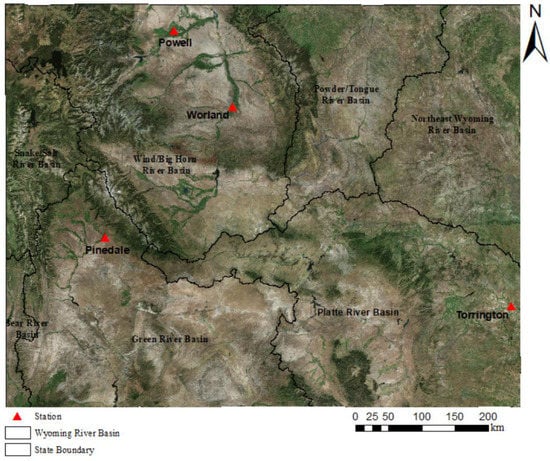
Figure 1.
Major river basin regions and the location of selected stations in Wyoming.
Climate data for the analysis were obtained from four weather stations near Powell, Worland, Pinedale, and Torrington, Wyoming (Table 1; Figure 1). Stations were selected based on data availability, period-of-record (>50 years), and proximity to agricultural lands. The different study period for different stations was selected to quantify the long-term trend and to compare the difference between the current situation and the Dust Bowl Era drought (1930−1935). In addition, the long-term trend for the common period (1963–2017) when data for each station is available were also discussed for potential differences among selected stations. These stations are operated by the National Weather Service (NWS) in manual mode, with observations made and recorded daily by an observer. All of these NWS stations have daily data for Tmax, Tmin, Tavg, and P. It is important to note, however, that the NWS site at Worland has undergone a few moves during its history and, even more so, was initially installed in an industrial setting. Automated stations were established near the NWS site in Powell in 2010 and near the NWS site in Worland in 2013. For the NWS site in Pinedale, the nearest automated station was installed in 2011, 15 km southeast in Boulder, WY. For the NWS site in Torrington, WY, an automated weather station was installed nearby in September 1996 and then moved to Lingle, WY, (15 km northwest) in May 2008. The automated weather stations are operated and maintained by the Wyoming State Engineer’s Office and the University of Wyoming Water Resources Data System’s (WRDS) Wyoming Agriculture Climate Network (WACNet). WACNet is an automated climate network that records hourly and daily climate variables [31]. The data from WACNet stations near the four NWS sites were used to model wind speeds. For the NWS climate data, there are data gaps in the observed Tmax, Tmin, and P, which were infilled according to the procedures outlined in Cropper and Cropper [32]. These include the following: (i) if data were missing for one day, the missing values were interpolated between the previous and following day; (ii) if temperature data were missing for more than one day and corresponding Tmin/Tmax values were available, then missing values were calculated based on the 11-year average of the Tmin/Tmax difference equal to the daily diurnal temperature range (DTR) of the missing day; and (iii) if both the Tmax and Tmin values were missing for more than one day, the values were calculated based on the 11-year daily average of the missing day. The 11-year average was used such that interpolated values equal the average of the decadal climate.

Table 1.
Weather station metadata for select weather stations used in the study.
2.2. Methods
Grass and Alfalfa Reference Evapotranspiration Calculation (ETo and ETr)
Reference evapotranspiration (ETref) was calculated on a daily time-step using the Standardized Penman-Monteith equation with a fixed surface resistance of 45 s m−1 and 70 s m−1 and fixed plant height of 0.50 m for alfalfa and 0.12 m for pasture grass [27] as follows:
where is standardized grass and alfalfa reference evapotranspiration (ETo and ETr) (mm d−1), is net radiation at the reference surface (MJ m−2 d−1), G is the soil heat flux density (MJ m−2 d−1), T is the mean daily air temperature (°C), is the mean daily wind speed at 2 m height (m s−1), is the saturation vapor pressure (kPa), is the mean actual vapor pressure (kPa), () is the vapor pressure deficit (kPa), Δ is the slope of the saturation vapor pressure curve (kPa °C−1), is the psychrometric constant (kPa °C−1), and are numerator and denominator constants that change with a reference surface and calculation time-step. accounts for the time-step, bulk surface resistance, and aerodynamic resistance of the reference surface. and coefficients are 900 and 0.34 for ETo, and 1600 and 0.38 for ETr, respectively, over a daily time-step.
In this study, measured Rs were available beginning in 2011 for the Pinedale station, 2010 for Powell, 1997 for Torrington, and 2013 for Worland. Earlier Rs data were calculated on a daily time-step following the Hargreaves and Samani [25] and Samani [33] approach using measured Tmax and Tmin data as:
where KT is an empirical coefficient, is daily extraterrestrial radiation (MJ m−2 d−1), and TD is the mean maximum and minimum temperature difference (°C). Daily and other associated variables and parameters were calculated as a function of day of the year, solar constant and declination, and latitude using the procedures presented by Duffie and Beckman [34]:
where is the solar constant of 0.0820 MJ m−2 min−1, is the latitude (rad), is the inverse relative distance from Earth to Sun, which is calculated as a function of day of the year (J) as:
is the sunset hour angle (rad), which was calculated as:
and is the solar declination angle (rad), which was calculated as:
The was calculated as the radiation balance between incoming net shortwave radiation and outgoing net longwave radiation [27] as:
The is calculated as the radiation balance between incoming shortwave radiation and reflected solar radiation as:
where α is surface albedo. In this study, a constant value of 0.23 is used for the analysis.
Net longwave radiation is calculated as:
where is Stefan−Boltzmann constant of 4.903E−9 MJ K−4 m−2 d−1, and are the daily maximum and minimum absolute temperature in Kelvin, is the actual vapor pressure (kPa), is incoming shortwave radiation, and is the clear sky solar radiation (MJ m−2 d−1), which is calculated as:
The daily soil heat flux (G) beneath the reference grass and alfalfa surface is generally small, so it was neglected for 24-hour time-steps. Actual vapor pressure () was calculated as:
is the dew point temperature (°C); however, in the absence of data, many studies assume minimum daily temperatures are in equilibrium with . This assumption is an acceptable approximation under clear sky conditions in sub-humid to humid climates. However, in Wyoming’s semi-arid climate, this assumption might not always be valid. In this study, was calculated by subtracting a temperature-dependent term from daily minimum temperature (), following the procedure developed by [35]:
where is diurnal temperature computed from daily and as:
The coefficient k is a calibration coefficient that accounts for site-specific tendency for RH below 100%. Values for k were computed on a monthly basis using measured RH data for each automated weather station (Figure 2). Due to a lack of RH data at the Worland station, k values from the Powell station were used to calculate Tdew. Missing RH data were calculated as the ratio of actual vapor pressure ( to saturation vapor pressure () at the same air temperature as follows:
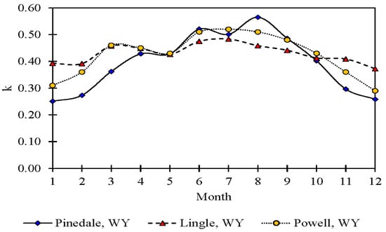
Figure 2.
Monthly variation in calibration coefficient (k) for the Tdew calculation. Coefficient k account for the site-specific tendency of relative humidity to remain below 100%.
The was calculated from measured values of and . The slope of saturation vapor pressure versus air temperature (Δ) was calculated as a function of air temperature following [27].
Wind speed measurement at 2 m height (u, m s−1) is an essential component of the standardized Penman−Monteith equation. Measured wind speed measurements at 3 m height, beginning in 2011 for Pinedale, 2010 for Powell, 1997 for Torrington, and 2013 for Worland were converted to u using the logarithmic function [27]. When data were not available, u was estimated following Curtis and Eagleson [36]. Details of this estimating procedure are provided in Appendix A.
To further understand the impact of climate variables on ETref, linear regression models were developed to evaluate the relationship between ETo and ETr with Tmax, Tmin, Tavg, P, Rs, Rn, u, VPD, and RH. For each climate station, the coefficient of determination (R2) was used to measure the proportion of variability in ETo and ETr explained by the climate variables. Furthermore, variations in ETref can be caused by both radiometric and aerodynamic variables [27]. Changes in the radiative component can be explained by contributions from Rn and Δ, whereas changes in the aerodynamic component can be explained by VPD, u, and Δ contributions. We divided the ETo and ETr equations into their aerodynamic and radiative components, as follows, to evaluate the contribution of each to total ETo and ETr:
2.3. Statistical Analysis
2.3.1. Homogeneity Analysis
Three non-parametric methods (i) Pettitt Test (PT) [37], (ii) Alexandersson’s Standard Normal Homogeneity Test (SNHT) [38], and (iii) Buishand’s Range Test (BRT) [39] were employed to detect any significant TCP in the measured data time-series. All of the three tests used in this study assume the null hypothesis of data being homogeneous; i.e., no change point exists in the time series. These tests were selected because of their different characteristics; for example, the SNHT test is more sensitive to inhomogeneities in the beginning and later end of the time series, whereas PT and BRT tests work better in identifying the TCP near the middle of time series. In this study, the TCP was investigated for only the measured climate dataset i.e., Tmin, Tmax, and P time series.
2.3.2. Trend Analysis
In this study, two non-parametric methods, the Mann−Kendall (MK) trend test [40,41] and Theil−Sen’s slope estimator [42,43], were used to detect long-term trends in climate variables. The MK test’s null hypothesis states that datasets are independent and identically distributed random variables (i.e., there is no trend or serial correlation among the data series). The alternative hypothesis states that the data follow a monotonic trend. However, in many cases, the observed dataset is auto-correlated (e.g., Tmax and Tmin), which may result in misinterpretation of the trend analysis [44,45]. For example, a positive serial correlation results in wrongful rejection of the null hypothesis of no trend when it is true (type I error). Similarly, a negative serial correlation results in accepting the null hypothesis of no trend when it is false (type II error). To eliminate potential issues in time series data, a modified MK test was used by removing the lag-1 serial correlation component from the time series. This process is called pre-whitening. The lag-1 serial correlation of sample data (k = 1) was computed as [44,45]. The “modifiedmk” open-source library package in R-language was used to perform all the non-parametric MK tests, Theil-Sen’s Slope test, and all modified versions of MK test mentioned in this study.
3. Results and Discussion
3.1. Trends in Climate Variables
3.1.1. Maximum, Minimum, and Average Temperatures (Tmax, Tmin, and Tavg)
Long-term fluctuations in air temperature can cause distinct changes in ETref, influencing agricultural water consumption patterns and production outcomes. Because of its high elevation, Wyoming has a relatively cool climate. Table 2 presents descriptive statistics of Tmax, Tmin, and Tavg for Pinedale, Powell, Torrington, and Worland, WY over the study period, and from 1963–2017. Over the period-of-record, a maximum average annual Tavg of 8.7 °C (range: −0.01 to 17.4 °C) was observed for Torrington, WY, and a minimum average annual Tavg of 2.3 °C (range: −6.4 to 10.9 °C) was observed for Pinedale, WY. At all the stations, January and July were the coldest and warmest months (data not shown). From 1963–2017, Tvag was 73%, 14%, and 13% and Tmax was 36%, 12%, and 9% higher for Torrington compared to Pinedale, Powell, and Worland, respectively. For the same period, minimum Tmin was 96%, 98%, and 87% lower for Pinedale than forPowell, Torrington, and Worland, respectively.
Table 2.
Average values with standard deviation for climate variables used in this study from four weather stations over the period-of-record and from 1963–2017. Tmin, Tmax, and Tavg = minimum, maximum, and average air annual temperature, respectively (°C); P = average annual precipitation (mm); Rs and Rn = average annual incoming shortwave radiation and net radiation, respectively (MJ m−2 d−1); u = average annual wind speed at 2 m height (m s−1), VPD = vapor pressure deficit (kPa); RH = relative humidity (%); MinTmin = minimum annual minimum temperature (°C); MaxTmin = maximum annual minimum temperature (°C); MinTmax = minimum annual maximum temperature (°C); and MaxTmax = maximum annual maximum temperature (°C).
Annual distribution in Tmax, Tmin, and Tavg for the period-of record and common period (1963-2017) along with trend lines is presented in Figure 3. Over the period-of-record, significant positive long-term trends (p−values < 0.05) in Tmax, Tmin, and Tavg were observed at all stations, except Torrington, where there were no significant positive trends, and instead a significant negative trend in Tmax (Table 3). Total change in Tmax for the period-of-record was 1.2 °C, 0.9 °C, −1.2 °C, and 1.3 °C at Pinedale, Powell, Torrington, and Worland, respectively. Although there is a small decreasing trend in Tmax at Powell (−0.01 °C year−1) from 1963–2017, the recent warming trends (Tmax) at Powell and Worland are more pronounced than during the Dust Bowl Era in the 1930s. For example, from 1988 to 2017, a total change of 0.9 °C and 0.3 °C in Tmax was at Powell and Worland, respectively (Table 4). In addition, the maximum decadal changes in Tmax occurred between 1981–1990 for Powell (1.8 °C decade−1) and Worland (2.5 °C decade−1) (Table 4). This is due to an increasing frequency of the number of very hot days (days with Tmax > 35 °C) since 1980 at all stations (data not shown). On a seasonal time-step, significant positive trends in Tmax are observed for March to August, with a maximum change (p-values < 0.05) of +1.5 °C, +1.21 °C, and +1.6 °C for Pinedale, Powell, and Worland, respectively. In contrast, a significant negative Tmax trend was observed at Torrington for September to February, with a maximum decrease of −1.7 °C (Table 3).

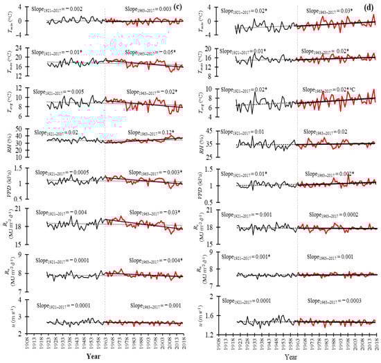
Figure 3.
Temporal variation in minimum, maximum, and average temperature (Tmax, Tmin, and Tavg; °C), relatively humidity (RH; %), vapor pressure deficit (VPD; kPa), incoming solar radiation (Rs; MJ m−2 d−1), net radiation (Rn; MJ m−2 d−1), and wind speed (u; m s−1) at 2 m height on an annual time–step for the period-of-record and the common period of 1963–2017 (red line) at (a) Pinedale, (b) Powell, (c) Torrington, and (d) Worland, Wyoming, with slope (yr−1). The asterisks (*) sign represents the significant trends at a 5% significance level. The dotted and solid black lines indicate the linear trend line for total data and the common period (1963–2017).
Table 3.
Theil-Sen’s slope (Qi) of the meteorological variables and grass and alfalfa reference evapotranspiration at annual and seasonal time-step for four weather stations in the state of Wyoming.
Table 4.
Magnitude of change (unit per 10-year, 1963–2017, and 1988–2017 period,) statistics (Theil-Sen Slope, Qi) of the meteorological variables at four weather stations in the state of Wyoming.
The significant negative Tmax trend in Torrington on annual and seasonal scales (especially from 1963–2017 (0.05 °C year−1) and 1988–2017 (−0.1°C year−1) (Figure 3; Table 3 and Table 4) might be due to the cooling effect of irrigation in southeast WY. For example, southeast Wyoming, where most of the agriculture is dependent on the groundwater resources from the Ogallala Aquifer, had a notable increase in groundwater withdrawal for irrigation by 180 million gallons per day from 2005 to 2015 [46]. However, the relationship between irrigation expansion and its effect on local and regional temperature trends is beyond the scope of this study. A similar negative trend in Tmax was observed by Lobell and Bonfils [47] at the irrigated sites in California during June–August, owing to irrigation expansion in the region. Analysis of long-term climate observations and climate and land surface modeling efforts by Mahmood et al. [48] and Kueppers et al. [49] have shown that irrigation can consistently reduce Tmax. A similar negative trend in Tmax was also observed by Sharma et al. [10] in Panhandle, NE, which is in the same climate zone as Torrington, WY. They reported that the negative trend in Tmax is due to the expansion of irrigated acres in western NE, which may have contributed to increased atmospheric moisture and cloudiness, resulting in a decrease in Tmax.
Over the period-of-record, statistically significant increases in Tmin (p-value < 0.05) at the annual time-step were observed for all stations, except Torrington (Table 3). The degree of observed changes for Tmin over the period-of-record was 2.20 °C, 0.66 °C, −0.19 °C, and 1.84 °C at Pinedale, Powell, Torrington, and Worland, respectively. Similar to Tmax, a negative trend in Tmin from 1963-2017 at Powell is mainly due to a drop in Tmin from 1977 to 1986, which led to the overall decreasing trend from that period and thereafter (1988–2017), and a significant positive trend was observed (Table 4). For example, the total change in Tmin from 1988 to 2017 was 1.2 °C, 1.8 °C, −0.09 °C, and 0.6 °C at Pinedale, Powell, Torrington, and Worland, respectively. In addition, for all stations, the largest decadal changes in Tmin also occurred in the same period, with a total change of +1.50 °C, +1.80 °C, and +2.3 °C decade−1 from 1990–2017, except the Powell station, where the maximum decadal change in Tmin of 3.0 °C decade−1 occurred in the Dust Bowl Era of 1930–1940 (Table 4). Recent increases in Tmin at Pinedale, Torrington, and Worland illustrate the decreasing frequency of the number of cold days (daily Tmax < 0 °C) starting in the 1980s. Similar to Tmax, statistically significant increases (p-value < 0.05) were observed for all seasons at Pinedale and Worland, with maximum Tmin increasing by +2.8 °C for December, January, and February (DJF) and 3.3 °C for March, April, and May (MAM). For Powell, with the exception of September, October, and November (SON), there is a positive trend for all other seasons, with the highest Tmin increase of 1.1 °C in the months of MAM (Table 3). Over the period-of-record, Tavg showed a significant positive trend at Pinedale, Powell, and Worland and a significant negative trend at Torrington (Table 3). Although a significant increasing trend was observed in Tavg in recent years (1988–2017), the decadal trend in Tavg revealed that for both Powell and Worland, the warming trend is much more pronounced than in the Dust Bowl Era in the 1930s (Table 4). The largest change in Tavg is +0.04 °C at Pinedale and +0.01 °C year−1 at Powell, both observed in MAM, and −0.02 °C at Torrington and +0.02 °C year−1 at Worland, both observed in DJF.
It is important to note that climate change may not always be characterized by changes in the means of climate variables, but rather by changes in parameters such as standard deviation, skewness, or median and mode [21]. To further understand positive and negative trends in Tmax and Tmin, annual minimum and maximum values of Tmin and Tmax (MinTmin, MaxTmin, MinTmax, and MaxTmax) were analyzed (Table 2 and Table 3). Increases in Tmax and Tmin values at Pinedale, Powell, and Worland are accompanied by significant increases in MinTmin and MaxTmax both over the study period as well as in recent years (1988–2017). This study indicated that MinTmin is rising at a faster rate than MaxTmax. These increases suggest that cooler days and nights, along with frosts, have become less frequent, while hotter days and nights, along with heat waves, have become more frequent. Significant negative trends in annual Tavg and Tmax at Torrington are due to significant decreases in MinTmax, which overshadows the effect of significant positive seasonal trends in MinTmin in December through May. In addition, in recent years (2000 to 2017), approximately 59%, 59%, 65%, and 76% of years at Pinedale; 76%, 53%, 65%, and 65% of years at Powell; and 49%, 29%, 59%, and 88% of years at Worland have higher values of MinTmin, MaxTmin, MinTmax, and MaxTmax than their long-term average values, illustrating warming trends in recent years.
The climatic forces responsible for warming in WY are complex and are not fully understood. Many factors could lead to the recent warming (e.g., the elevation dependency of warming, which is most likely due to the combined effects of cloud radiation and snow-albedo feedback, changes in atmospheric circulation, and land-use changes). The significant increase in winter and summer air temperature observed in this study is likely to result in increased winter runoff, reduced peak snow-water equivalent, earlier peak streamflow, and reduced summer streamflow volumes [50]. Agriculture is one of the important economic activities in the state. Crops such as alfalfa, sugarbeet, dry bean, and barley grown in Wyoming are highly dependent on the irrigation practices, which is highly dependent on the winter snowpack accumulation. Continued increase in Tmax and Tmin in recent years especially in the northwestern and western parts of the state will have a significant effect on the water supply and soil moisture availability in the region, which can further affect the irrigate agriculture.
Similar 21st century warming trends on annual and seasonal time-steps are reported by Frankson et al. [51] in Wyoming with net warming of 1.4 °C since the beginning of the 20th century. They concluded that since 2000, the state has experienced above-average frequency of extremely hot days and below-average frequency of extremely cold days. These results also align with those observed by Gaffen and Ross [52], who reported an increase of over 0.4 °C decade−1 from 1961 to 1995 in the High Plains. Similar results were obtained by Hamlet and Lettenmaier [53] over the western U.S. They used the Historical Climatology Network (HCN) and Historical Canadian Climate Database (HCCD) data, which showed greater increases in minimum temperatures compared to maximum temperatures. A similar observation was made by Mote [54] in the Pacific Northwest U.S. and reported an increase of 0.7 °C to 0.9 °C in annual averaged air temperature from global averages. In the same regions, Abatzoglou et al. [55] observed an accelerated warming rate with linear trends for the 1970–2012 and 1980–2012 time periods of approximately 0.2 °C decade−1. Temperature trends observed in this study are also consistent with Santos et al. [56]. They used Tmax and Tmin temperatures data taken from 35 meteorological (weather) stations across Idaho, U.S. and observed that the difference between Tmax and Tmin is decreasing, indicating that the Tmin is increasing faster than the maximum air temperature. The increasing trend in air temperature observed in the study is also consistent with the findings of Karl et al. [57] and Meehl et al. [58]. The results observed in this study at Pinedale are also consistent with Hall et al. [59], who showed a pronounced statistically significant increasing trend in Tmax and Tmin in the spring and summer months at Pinedale, Wyoming.
3.1.2. Precipitation (P)
Changes in P regimes indirectly have a significant effect on other climate variables and thus ETref. Figure 4 represents the annual variation in P for Pinedale, Powell, Torrington, and Worland. Like other locations in the western U.S., annual P varies greatly by location and from year to year. Being a headwaters state, Wyoming serves as a major source of water for several downstream states, so changes in P can have broad implications beyond the state’s boundaries. The long-term average annual P over the study duration was 292 ± 72, 160 ± 46, 351 ± 83, and 199 ± 62 mm at Pinedale, Powell, Torrington, and Worland, respectively, with 51%, 55%, 51%, and 56% of the years having below-average P. Powell and Worland stations in the Big Horn Basin experience less P than the other stations, likely due to the effect of multiple mountain ranges blocking the flow of moist air from both the east and west.
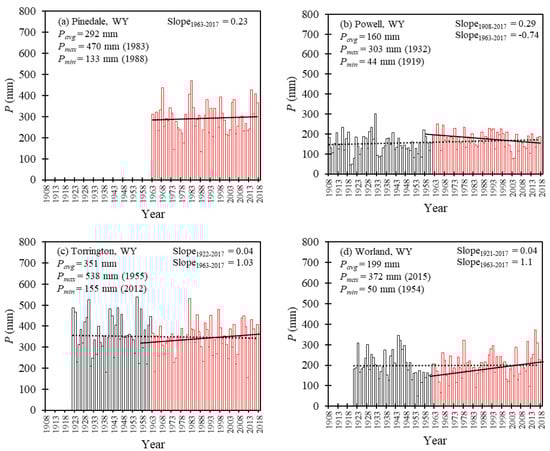
Figure 4.
Variation in annual total precipitation (P, mm) at (a) Pinedale, (b) Powell, (c) Torrington, and (d) Worland, Wyoming. The dotted and solid black lines indicate the linear trend line for total data and the common period (1963–2017).
Over the study duration, all stations except Torrington show a positive trend in either annual or seasonal P. There was approximately 12.5, 31.6, −3.9, and 4.1 mm of change in annual P over the study duration at Pinedale, Powell, Torrington, and Worland, respectively. At Powell and Worland, there was a significant positive trend in P during the spring (MAM). Pinedale instead experienced a significant positive trend in P during the fall (SON), as well as a significant negative trend during the summer (JJA). The positive trend in spring P is due to the rising spring temperatures that cause an increase in the snow line (the average lowest elevation at which snowfalls). This further increases the likelihood that some of the snow will fall as rain, which can reduce water storage in the form of the snowpack, particularly at lower elevations. Heavy spring month P, along with increased spring temperatures, can cause severe flooding by causing the rapid melting of the snowpack, further decreasing water availability during the drier summer months [53]. On a seasonal scale, JJA P (representing the crop-growing season months) shows the largest negative trend for all stations, except Powell, WY, where seasonal P shows a positive trend. For the period-of-record, a maximum change of −32 mm (Pinedale, WY), +18.4 mm (Powell, WY), −9.2 mm (Torrington, WY), and −24.5 mm (Worland, WY) was observed for the JJA period. On a decadal scale, the largest change in precipitation occurred in 1981–1990 (−23.9 mm decade−1) at Pinedale, 1931–1940 (+11.5 mm decade−1) at Powell, 1922−1930 (+33.5 mm decade−1) at Torrington, and 1961–1970 (−10.9 mm decade−1) at Worland. In addition, increases in P were observed in recent years (1988–2017) at all stations except Powell, with an annual average P change of 36, −48, 26, and 12 mm was observed at Pinedale, Powell, Torrington, and Worland, respectively. The seasonal trends of increasing P in spring and decreasing summer P in some Wyoming stations are consistent with other studies in the region [52,54,55,60,61].
3.1.3. Incoming Shortwave Radiation (Rs) and Net Radiation (Rn)
Incoming solar radiation (Rs) and net radiation (Rn) are excellent estimators of the radiative budget for ETref. However, in many cases, these datasets are not available for long-term analysis. Over the years, many models have been developed to estimate Rs ranging from simple models that are based on sunshine duration, cloud cover, and temperature extremes to more complex models that require detailed meteorological data such as u, RH, and Tdew [62,63,64,65,66]. Sanchez et al. [63] and Sanchez-Lorenzo and Wild [64] estimated Rs based on a homogeneous sunshine duration series to study the long-term (1885−2010) trend in Rs in Spain and Switzerland, respectively. Biggs et al. [65] estimated Rs using a combination of the Angstrom equation and the modified Hargreaves equation to study the trend in Rs in southern India from 1985−1997. Similarly, Bandyopadhyay et al. [66] compared different models to estimate Rs and observed that the original Hargreaves method performs better than other methods. Therefore, in this study, due to the limitation of Rs and Rn data availability, Rs was modeled on a daily time-step using the Hargreaves and Samani [18] approach. Rn was calculated as the radiation balance between incoming net shortwave radiation and outgoing net longwave radiation. It is important to note the modeling of Rs from air temperature and extraterrestrial radiation has some error that can impact the trend and magnitude of changes in ETref. To check the accuracy of the modeled Rs values, the estimated values were compared with available Rs values for each station. At all stations, the model overestimates in the lower Rs range. In general, the Rs estimates are within 10% (overestimated) of the measured values. Overall modeled estimates of Rs compare well with the station data, with high Pearson’s correlation coefficient (R2) and small root mean square difference (RMSD) R2 = 0.77, RMSD = 3.99 MJ m2 d−1 at Pinedale; R2 = 0.84, RMSD = 3.33 MJ m2 d−1 at Powell; R2 = 0.71, RMSD = 4.76 MJ m2 d−1 at Torrington; R2 = 0.79, RMSD = 4.15 MJ m2 d−1 at Worland (Figure S1). The relationship between the estimated and measured Rs improved when it is accounted for at monthly and yearly time−step. It was observed that a 10% increase in Rs yielded between 2.8% and 3.9% increase in ETo and between 6.5% and 6.7% increase in Rn at all sites. A similar observation was made by Irmak et al. [21], who observed that overestimation in Rs would impact the Rn value portion of the ETref estimates. They found that an 8% overestimation of Rs would result in a 2% and 6.4% overestimation in ETref and Rn, respectively, with all other climate variables held constant. A similar observation was made by Bandyopadhyay et al. [66], who found a relatively small effect of modeled Rs on ETo estimates over 29 stations distributed throughout India. While the overestimation in modeled Rs may have a minor impact on the magnitude and long-term trend of ETref, it is not large enough to impact the annual average trend of Rn and ETref in this study.
The annual average Rs over the study duration at Pinedale, Powell, Torrington, and Worland was 18.4 ± 0.5, 16.7 ± 0.4, 18.4 ± 0.6, and 17.7 ± 0.4 MJ m2 d−1, respectively (Table 2). Overall, annual Rs follows a significant positive trend at Powell, and a negative trend at Pinedale, Torrington, and Worland (Table 3). Total change in Rs over the period-of-record was −0.5, +0.3, −0.4, and −0.1 MJ m−2 d−1 at Pinedale, Powell, Torrington, and Worland, respectively. On a seasonal scale, statistically significant increases in Rs occurred mainly during summer and fall (JJA and SON) (Table 3). Time series analysis of Rs from 1963 to 2017 revealed mixed results with an increasing Rs trend in Powell and Worland and a negative trend in Pinedale and Torrington, with a total change of −0.5, +0.2, −1.7, and +0.01 MJ m−2, d−1, respectively (Table 4). However, all the positive trends turn negative from 1988 to 2017 time period. Rn follows a similar trend as Rs, with the exception of Torrington where Rs and Rn have inverse trends, particularly in the months of SON and DJF. The negative trend in Rs and Rn at the Pinedale station is characterized by cloudier skies when compared to the Powell and Worland stations, where clear skies increase Rs and Rn, resulting in higher Tmax and Tmin values.
3.1.4. Wind Speed (u)
Wind speed at 2 m height (u) remains relatively constant throughout the period−of−record for all stations (Table 4), with minor seasonal fluctuations (Table 3, Figure 3). It is important to note that although we presented the trends in u, it is not anticipated because in modeling u (based on the availability of station data), the mean and variance remain relatively constant based on time of day, which preserves skewness and distribution [36]. Because the model uses simulated u, independent of other climate variables, the trend in modeled u does not exhibit any bias when compared to measured station data at all locations, indicating the accuracy of the modeling algorithm used. In addition, the estimated u values are comparable to the measured wind speed data at all stations (Figure 5). In all cases, mean, variance, lag−1 value of autocorrelation, and skewness of simulated u are in agreement with the measured data (Figure 5). Similarly, positive skewness in the frequency distribution of u was observed by Ivanov et al. [67], with mean observed and simulated u of 3.49 and 3.26 m s−1, respectively, for Albuquerque. Over the study duration, average annual u of 2.05 m s−1 (range: 1.84 to 2.21 m s−1), 2.65 m s−1 (range: 2.39 to 2.91 m s−1), 1.75 m s−1 (range: 1.57 to 1.95 m s−1), and 1.48 m s−1 (range: 1.34 to 1. m s−1) were observed for Pinedale, Torrington, Powell, and Worland, WY, respectively (Table 2). While our analyses did not consider the annual trends in u, Xie and Zhu [68] observed a decreasing trend in u at higher altitude state of Tibetan Plateau from 1970 to 2009, with u decreasing at a rate of 0.21 m s−1 decade−1. A similar decreasing trend in u was observed by Yin et al. [69] with u decreasing at a rate of 0.09 m s−1 per decade in China. In the Central High Plain Region of Nebraska, Sharma and Irmak [10] reported an overall reduction of 0.94 and 0.67 m s−1 on annual (January–December) and seasonal (May to September) time-steps, respectively, from 1986 to 2009. In theory, a decrease in u would cause ETref to decline, with all other climate variables remaining constant; however, this rarely occurs. It was observed with 1% decrease in daily average u yielded between 0.17–0.3% decrease in ETref. A similar observation was made by Irmak et al. [21], who reported that the effect o u on ETref can easily be obscured by changes in other climate variables, especially changes in Rs.
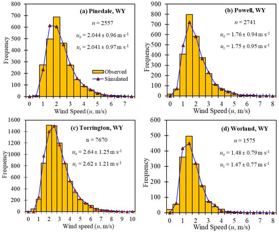
Figure 5.
Histogram of daily wind speed (u, m s−1) from observed and simulated data for (a) Pinedale, (b) Powell, (c) Torrington, and (d) Worland, Wyoming. The u0 and us represent the mean and standard deviation for observed and simulated data.
3.1.5. Relative Humidity (RH) and Vapor Pressure Deficit (VPD)
The annual change of average relative humidity (RH) and vapor pressure deficit (VPD) over the study duration and for the common period (1963–2017) are presented in Table 3. In this study, both RH and VPD are calculated from Tdew, which in turn is estimated using Equations (3) and (4) and is based on the availability of measured RH data from each station. On a daily time-step, the relationship between estimated and measured Tdew is strong (R2 = 0.86; RMSD = 4.2 °C for Powell weather station (Figure S2)). In general, relatively low RH values were observed at all stations (Table 2). On an annual scale, RH values increase over the period-of-record for Pinedale, Torrington, and Worland stations and decrease at the Powell station (Table 3). This trend remains the same from 1963–2017 for all the stations. At Powell, there is a significant decline in RH of 7.3% from 1922−1930 and 4.5% from 1971−1980, followed by an increase of 3.6% from 1988–2017 (Table 4). At the Worland station, RH increased by 5.9% from 1951–1960 but then decreased by 9.4% from 1981−1990.
In theory, VPD decreases with increasing precipitation; however, under the semi−arid conditions of Wyoming, a small increase in precipitation has very little effect on VPD relative to the influence of and variation in u, Tmax, and Tmin. For all stations except Torrington, VPD follows a significant (p-value < 0.1) positive trend on an annual scale over the study duration as well as in recent years (Table 3). Over the period-of-record, VPD increased at a rate of 0.001 kPa year−1 at Pinedale, Powell, and Worland, and decreased at a rate of −0.001 kPa year−1 at the Torrington station. Similar to annual trends, significant increases in the VPD trend are observed for JJA (crop growing season) for all stations (0.02 kPa year−1), except at Torrington, where no trend was observed. No visible trend at Torrington is likely due to continuous fluctuation in VPD at the decadal time−step with sharp upward shifts from 1931–1940 (0.2 kPa decade−1) and 1981−1990 (0.2 kPa decade−1) and a sharp decline in 1971–1980 (−0.2 kPa decade−1) (Table 4).
3.2. Trend Change Point (TCP) Analysis
In long-term climatic trend analysis, identifying the trend along with the time of trend changes plays an important role. In this study, three non-parametric tests PT, SNHT, and BRT [37,38,39] were employed to detect any significant TCPs in the measured data time-series (Tmin, Tmax, and P) on both annual and seasonal scales. On average, similar results were observed from the three tests used in this study. Test results revealed significant TCPs in Tmax and Tmin time-series data; however, no TCPs were observed for the P time series at all stations on annual and seasonal scales (Table 5). For Pinedale, significant TCP occurred in 1993 for the annual Tmin data series. On a seasonal scale, TCP in the Tmin data series occurred in 1993 for winter months (DJF) and 1980 for summer and fall months (MAM and JJA). At Powell, significant TCP occurred in 1937 and 1951 for Tmin and Tmax, respectively, on an annual scale. On a seasonal scale, TCP was mainly observed during the 1950s and 1980s (Table 5). For Torrington, TCP was observed only for Tmax, with a change point that occurred in the late-1970s and mid-2000s. For Worland, the TCP occurred in the late-1970’s for both Tmax and Tmin on annual and season scales. As stated by Alexandersson and Moberg [39], there are many reasons for trend change points, such as relocation of the station, instrument/sensor change, land-use, and management changes, or sudden changes in the environmental condition. For example, in this study, the site at Worland has undergone a few moves during its history, especially in late 1970s, which is also reflected in the change point analysis for both Tmax and Tmin. Similarly, the recent trend change point at Torrington (mid−2000s) may also be due to a significant increase in water use for irrigation. For example, southeast Wyoming, where most of the agriculture is dependent on the groundwater resources from the Ogallala Aquifer, had a notable increase in groundwater withdrawal for irrigation by 180 million gallons per day (43% increase) from 2005 to 2015 [46].
Table 5.
Significant Trend Change Points (TCP, years) identified by Pettitt’s Test (PT), Alexandersson’s Standard Normal Homogeneity Test (SNHT), and Buishand’s Range Test (BRT) at Pinedale, Powell, Torrington, and Worland on an annual and seasonal time scale.
3.3. Trends in Reference Evapotranspiration (ETref)
Estimates of atmospheric evaporative demand of reference grass and alfalfa surfaces (ETo and ETr), based on climate station data over the study duration at annual and seasonal scales, are presented in Table 6. It is important to note that estimated climate variables have some impact on the trend analysis and magnitude of changes of ETref. To check the accuracy of the ETref values calculated using the modeled variables, the estimated ETref values were compared to the ETref values when calculated using the measured full climate dataset at all four sites (Figure 6). Overall, a good relationship was observed between two approaches, with R2 values varying between 0.86 to 0.97 and RMSD ranging from 0.37 to 0.91 mm d−1. Maximum ETo values were observed in the years 1988, 1931, 1939, and 1981 at Pinedale, Powell, Torrington, and Worland, respectively. Their minimum ETo values were observed in the years 1993, 1924, 2009, and 1932, respectively. Comparing ETr and ETo at each station, average annual ETr values were 26%, 25%, 30%, and 25% higher than ETo at Pinedale, Powell, Torrington, and Worland, respectively. Greater fluctuation in both ETo and ETr was observed at each station, with 49%, 55%, 49%, and 53% of years having above−average ETo for Pinedale, Powell, Torrington, and Worland, respectively, and 51%, 56%, 45%, and 52% of the years had above-average ETr. For each station except Pinedale, maximum and minimum ETo and ETr values occurred in the same years that maximum and minimum Rs values occurred.
Table 6.
Descriptive statistics for annual and seasonal grass and alfalfa reference evapotranspiration (ETo and ETr, mm) for four weather stations in the state of Wyoming.
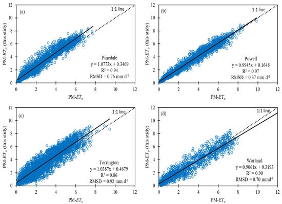
Figure 6.
Comparison of reference evapotranspiration (ETo, mm d−1) estimated using modeled variables Penman−Monteith (PM)–ETo (this study) against the Standardized Penman−Monteith estimated reference evapotranspiration (FAO-56) estimated using full measured climate dataset at (a) Pinedale (2011 to 2017), (b) Powell (2010 to 2017), (c) Torrington (2008 to 2017) and (d) Worland (2014−2017).
On a seasonal scale, maximum ETo and ETr values were observed in JJA, and minimum values were observed in DJF (Table 6). At both seasonal and annual time-steps, comparison among the stations for the common time interval (1963 to 2017) reveals larger ETo and ETr values at Torrington, followed by Worland, Powell, and Pinedale. On average, Torrington’s annual ETo values were 23%, 22%, and 21% higher than those at Pinedale, Powell, and Worland. Similarly, Torrington’s annual ETr values were 27%, 26%, and 26% higher than those of the other stations. Higher ETo and ETr values at Torrington are due to higher values of Tmax, Tavg, Rs, u, and VPD compared to the other stations for the same time interval (1963−2017). For example, annual Tavg at Torrington was approximately 73%, 14%, and 13% higher than Tavg values at Pinedale, Powell, and Worland, respectively. Similarly, average annual VPD was approximately 32%, 13%, and 4% higher at Torrington compared to other stations. On daily time−steps, histograms of ETo and ETr for each station (Figure 7) are positively skewed with the peak (i.e., mode) values between 0 to 1 mm d−1 for ETo and 1 to 2 mm d−1 for ETr. However, at Torrington, peak (i.e., mode) ETo and ETr values are observed between 1 to 2 mm d−1 and 2 to 3 mm d−1 (Figure 7). Average daily values of 3.0, 3.9, 3.0, and 3.1 mm for ETo and 4.1, 4.2, 5.6, and 4.1 mm for ETr were observed at Pinedale, Powell, Torrington, and Worland, respectively.
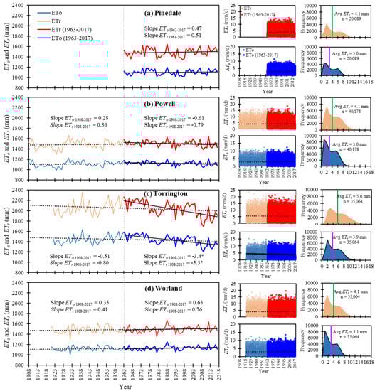
Figure 7.
Temporal variation of grass and alfalfa reference evapotranspiration (ETo and ETr, mm) at annual and daily time scale over the period−of−record and from 1963−2017 along with histogram distribution of daily ETo and ETr at (a) Pinedale, (b) Powell, (c) Torrington, and (d) Worland, WY. (Pink and green lines in the histograms represent the mean daily ETr and ETo, respectively.)
A time-series graph of grass− and alfalfa-based reference evapotranspiration (ETo and ETr) on an annual and daily time-step (Figure 7) suggested positive trends in both ETo and ETr at Pinedale, Powell, and Worland but negative trends at Torrington. Over the study duration, an overall change of +26, +31, −48, and +34 mm in ETo was observed at Pinedale, Powell, Torrington, and Worland. Likewise, an overall change of +28, +40, −80, and +39 mm in ETr was observed. However, long-term trends at the annual scale were statistically significant only for ETo, and only at Powell and Worland (p-value < 0.1). No annual trends were statistically significant at the other stations, nor for ETr. A similar non-significant slight upward trend in ETr was observed by Clifford and Doesken [70] in Colorado from 1993 to 2007. Positive trends in annual ETo at Powell and Worland are associated with significant positive trends in annual P, Tmax, Tmin, and Tavg, Rs, and VPD and a significant negative trend in annual RH.
On a seasonal scale, Powell and Worland showed significant positive trends for both ETo and ETr during MAM, as well as significant positive trends during JJA for ETo (Table 3). Pinedale shared this significant positive trend during JJA, for both ETo and ETr. The total increase during JJA over the study duration was 26, 1.8, and 22 mm in ETo at Pinedale, Powell, and Worland, respectively. These positive trends in ETo and ETr during spring or summer were all associated with significant increases in Tmax and Tavg during those seasons. Other studies have detected significant increases in Tavg as the main cause of increasing ETo (e.g., [16]). A similar increasing trend in spring and summer ETo was observed by Hamlet et al. [71] with a median trend of 7–13 mm decade−1. They associated this increase with a rising vapor pressure deficit from July to September. Additional contributing factors at some of the stations included significant seasonal increases in Tmin, Rs, Rn, u, and VPD (Table 3). These trends imply that crop water requirements will likely increase in these regions because of increases in ETo and ETr during the growing season. If accompanied by decreases in summer precipitation, as observed in Pinedale for JJA (Table 3), these two combined effects could have adverse consequences for agricultural production. These increase trends in ETo and ETr, and its adverse consequences to agriculture have also been reported by Jaksa and Sridhar [72]. They used the Noah land surface model to study the long−term trends of ETc within the irrigated region of Snake River basin, Idaho for the past 30 years spanning between 1980 and 2010 and reported that warming climate and boundary-layer meteorological variables indicated that cooling induced by irrigation are the main cause of the increasing trend in ETc (increase at a rate of 0.78 mm year−1) in the region.
Torrington, in contrast to all the other stations, showed significant negative trends for both ETo and ETr, specifically during SON and DJF. These long-term decreases at Torrington may be the result of significant decreases in seasonal Tmax because of the cooling effect of irrigation [47,48,49]. In addition, a decreasing trend in ETref may be due to the decreasing trend in P. Trend analysis from 1963 to 2017 (red and blue lines in Figure 7) revealed that both ETo and ETr are decreasing at a much faster rate at Powell and Torrington but increasing at Pindale and Worland. A total change of +26, −34, −187, and +35 in ETo and +28, −43, −291, +42 mm in ETr was observed at Pinedale, Powell, Torrington, and Worland, respectively, from 1963–2017. Torrington’s trends are consistent with the findings of Sharma et al. [10], who reported similar negative trends from 1986−2009 in Panhandle, NE, which is in the same climate zone as Torrington, WY. A similar negative ETo trend was observed in China [73], India [16], and the U.S. [21]. All these studies reported that the negative trends in Tmax are the prominent cause of reduction in ETo.
On a decadal scale, all four stations experienced a statistically significant increase in ETo (as well as in ETr at all stations expect Powell) from 1981−1990 (Table 4). The magnitude of these increases was 11.4, 5.3, 19.8, and 14.5 mm year−1 for ETo at Pinedale, Powell, Torrington, and Worland, respectively; similarly, increases for ETr were 18.4, 9.4 (not statistically significant), 31.4, and 24.0 mm year−1. Only Worland experienced a statistically significant decline in ETo and ETr, specifically from 1951−1960, with ETo changing at a rate of −11.3 mm year−1 and ETr changing at a rate of −20.2 mm year−1 (Table 4). This decade also saw significant declines in u and VPD and a significant increase in RH. Powell, which is just 120 km northwest of Worland, saw similar conditions during this decade, but the reductions in ETo and ETr were not statistically significant.
Furthermore, the trend and contribution of aerodynamic and radiative components of ETo and ETr revealed that, for both ETo and ETr, the aerodynamic component contributes more at all stations, ranging between 45% to 59% of the total ETo and 59% to 79% of the total ETr (Table 7). The maximum aerodynamic contribution to ETo and ETr was observed at Torrington. Trend analysis of these components illustrates a positive trend in aerodynamic and radiation components at all stations, except Torrington, where both components show negative trends. The positive trends of aerodynamic and radiative components at Pinedale, Powell, and Worland are driven by the increasing trend of radiative components (i.e., solar radiation and air temperature) and positive trend of aerodynamic components (i.e., u and VPD). Negative trends in both radiative and aerodynamic components of ETo and ETr at Torrington are mainly driven by negative trends in both temperature and u. Moreover, the negative trend of u at the Torrington station was more evident than at the other three stations, which have a positive ETo trend.
Table 7.
Average percent contribution and slope of trend analysis for the aerodynamic and radiative components of ETo and ETr at Pinedale, Torrington, Powell, and Worland, WY.
Daily estimates of ETo and ETr were analyzed for their potential to inform future estimates of actual crop ETc based on the two-step approach of FAO-56 for calculating crop coefficients (Kc). Values for the grass crop coefficient (Kco) and alfalfa crop coefficient (Kcr) are typically obtained by dividing ETc by ETo and ETr, respectively. Since Kco and Kcr coefficients are not interchangeable, this study analyzed the relationships between daily ETo and ETr (Figure S3). The results indicated that, in semi-arid WY, the ratio of ETo/ETr ranged from 0.70 to 0.75. The minimum value was observed for Torrington, while the other stations’ ETo/ETr values were very close to 0.75. These values are consistent with those of Irmak et al. [74], who evaluated ETr/ETo (reciprocal to that presented in this study) in other climate regions. For example, the values at Pinedale, Powell, and Worland closely match the values Irmak et al. [74] reported for Phoenix, AZ, which is categorized as arid, while the Torrington ratio resembled values reported for semi-arid Bushland, TX.
3.4. Relationship between ETr and ETo and Climate Variables
Small changes in meteorological variables can result in significant changes in ETref; therefore, these relationships should be further evaluated. Linear regression models were developed to evaluate the relationship between ETo and ETr with Tmax, Tmin, Tavg, P, Rs, Rn, u, VPD, and RH on an annual time-step over the period-of-record (Table 8). Positive and negative signs in Table 8 indicate whether the relationship is positive or negative between a climate variable and ETo and ETr. Results show that, for all stations, nearly all climate variables have a significant correlation with ETo and ETr (p−values < 0.01), with the exception of Tmin, u, and P (where they are grayed out in Table 8). Most variables are positively correlated with ETo and ETr, except P and RH, which show a negative correlation. Tmax, Rs, and VPD explain the maximum amount of variation in ETo and ETr values across all four stations. Results for Pinedale, for example, indicate that VPD explains approximately 87% of variability in ETo and 83% of variability in ETr, followed by Tmax (0.70 in ETo and 0.67 in ETr) and Rs (0.66 in ETo and 0.67 in ETr). Tmin and u are poorly correlated to ETo and ETr (Table 8). Similar observations occur at Torrington, which is at a similar latitude as Pinedale, with VPD, Rs, and Tmax accounting for ~80% of the variability in ETo and ETr. Negative relationships between ETref and P at Pinedale and Torrington are probably due to higher cloud cover there and decreases in Tmax, Rs, Rn, and VPD, all of which are generally associated with increasing P.
Table 8.
Coefficient of determination (R2) observed between grass and alfalfa reference evapotranspiration (annual ETo and ETr) and climate variables. Tmin, Tmax, and Tavg = minimum, maximum and average air annual temperature (°C); P = average annual precipitation (mm); Rs and Rn = average annual incoming shortwave radiation and net radiation (MJ m−2 d−1); RH = relative humidity (%); u = average annual wind speed at 2 m height (m s−1); VPD = vapor pressure deficit (kPa); (+) and (−) signs indicate a positive or negative relationship between climate variables and ETo and ETr).
At Powell and Worland, in the northwestern portion of the state, the effects of VPD, Rs, and Tmax on ETo and ETr are somewhat less than at the other stations (Table 8). VPD, Tmax, and Rs explain approximately 81%, 59%, and 51% of the variability in ETo at Powell, and 73%, 54%, and 50% of the variability in ETr at Powell. They explain 75%, 71%, and 54% of the variability in ETo at Worland and 68%, 66%, and 59% of the variability in ETr at Worland. Another difference observed at Powell and Worland is the significant correlation of Tmin and u with ETo and ETr, which explain 10−16% of the variability in ETo and ETr. The negative relationship between ETref and P is probably due to an increase in cloud cover and decrease in Tmax, Rs, Rn, and VPD, which is generally associated with increasing P. Significant relationships between u and ETref at Powell and Worland, but not Pinedale and Torrington, are likely due to the more arid climate of the northwestern region. In general, u influences ETref through its effects on moisture content of the air. For example, because of the arid climate of northwestern Wyoming, the saturated air above the surface is replaced by drier air, which increases VPD and hence ETref.
These findings are consistent with results reported by Maček et al. [75], who examined the trends and relationships between climate and ETo from 18 meteorological stations located in the temperate continental to mountain climate of Slovenia. The authors reported that Rs had the largest impact on ETo, followed by Tavg and VPD. These results are also in agreement with Irmak et al. [76], who evaluated different climate regions and reported that ETo is highly sensitive to VPD. It should be noted that changes in magnitude or trend of one climate variable cannot solely describe the variation in ETref. The results indicated that ETref did not respond well to Tmin; however, a significant increase in Tmin can indirectly increase trends in Tavg, which in turn affects VPD and ETref. Therefore, it is important to account for all climate variables collectively when analyzing variation in ETref by using combination-based energy balance models as opposed to models based solely on simplified temperature or radiation components. In addition, this also makes it important to understand and quantify the individual contribution of the climatic variables to the changes in ETo and ETr. Therefore, future studies will aim at the sensitivity analysis of ETo and ETr to the changes in climate variables. Future studies will also aim to evaluate the spatio−temporal variation in ETref and ETa in the inter-mountain region of Wyoming.
4. Conclusions
Information on long−term trends in climatic variables, reference evapotranspiration (ETref), and their relationship to each other is vital in the management of agricultural, water resources, and hydrological systems under variable and changing climate conditions. In this study, long−term trends for reference evapotranspiration (ETref) and climate variables that directly and indirectly impact ETref were evaluated over four sites in the intermountain state of Wyoming: Pinedale (1963–2017), Torrington (1922–2017), Powell (1908–2017), and Worland (1921–2017). In addition, the long-term trend for the common period (1963–2017) when data for each station areavailable was also discussed for potential difference among selected stations. ETref was calculated on a daily time-step using the combination-based energy balance Standardized Penman-Monteith equation. For all sites, the full climate dataset (Tmax, Tmin, RH, u, and Rs) to estimate ETref was available only for recent years. Earlier climate data were estimated using a previously developed practical and robust procedure using the observed Tmax and Tmin data on a long-term basis. It is important to note that estimated climate variables have some impact on the trend analysis and magnitude of changes; however, the impact is not expected to be large enough to influence the results on this study, especially when annual scales are considered. Non-parametric Mann-Kendall trend test and Theil-Sen’s slope estimator were used to determine the statistical significance of positive or negative trends in climate variables and ETref. Three non-parametric methods, (i) Pettitt Test (PT), (ii) Alexandersson’s Standard Normal Homogeneity Test (SNHT), and (iii) Buishand’s Range Test (BRT), were employed to detect any significant TCP in the measured data time-series. For the data influenced by serial correlation, a modified version of the MK test (pre-whitening) was applied.
A statistically significant positive trend in maximum, minimum, and average annual temperature (Tmax, Tmin, and Tavg, respectively) was observed at all stations, except for Torrington in the southeast part of Wyoming, where these temperature measures had negative trends. The study indicated that the recent warming trends are much more pronounced than during the 1930s Dust Bowl Era. For all the stations, no TCPs were observed for P; however, significant changes in trends were observed for Tmax and Tmin on both annual and seasonal timescale (Table 5). Over the study duration, an overall change of +26, +31, −48, and +34 mm in ETo and +28, +40, −80, and +39 mm in ETr was observed at Pinedale, Powell, Torrington, and Worland, respectively. Two of the four study sites—Powell and Worland—exhibited a statistically significant positive trend in annual ETref for grass (ETo), but not for alfalfa (ETr), over the period−of−record (Table 3). These increases were associated with significant positive trends in annual Tmax, Tmin, and Tavg and significant negative trends in relative humidity (RH). Our study indicates that minimum Tmin is rising at a faster rate than the maximum Tmax. These increases suggest that cooler days and nights, along with frosts, have become less frequent, while hotter days and nights, and heat waves, have become more frequent. The other two study sites—Pinedale and Torrington—exhibited no statistically significant trend in annual ETref for grass (ETo) or alfalfa (ETr) over the period-of-record. However, a statistically significant negative trend was observed for both ETo and ETr at Torrington from 1963–2017, where ETo and ETr are decreasing at a much faster rate of 3.4 mm year−1 and 5.3 mm year−1 compared to other stations. That said, three stations—Pinedale, Powell, and Worland—exhibited statistically significant positive trends in seasonal ETref during the spring (MAM) or summer (JJA). Torrington showed no statistically significant positive seasonal trends, instead experiencing statistically significant negative trends during the fall (SON) and winter (DJF) seasons. These long−term decreases in fall and winter ETo and ETr are associated with significant decreases in Tmax, Tavg, Rs, and in some instances decreased u and VPD and increased RH.
On an annual time−step, ETo and ETr are significantly and positively correlated with Tavg, Tmax, Rs, Rn, and VPD and significantly negatively correlated with RH (Table 8). Such increases in ETo and ETr, if combined with a decrease in summer (JJA) precipitation (e.g., at Pinedale), may have serious adverse consequences for agricultural production. Increases in ETo and ETr trends in MAM and JJA months could be attributed to increases in crop water requirements for the production of various crops and early snowmelt in mountainous regions that determine seasonal water availability. Therefore, it is important for state agencies, irrigation districts, and water managers to consider these rising trends when discussing future developments for water resources and agriculture in Wyoming, particularly given long-term warming trends in the state.
Supplementary Materials
The following are available online at https://www.mdpi.com/2073-4441/12/8/2159/s1, Figures S1–S3 are added as supplement material. Figure S1. Measured vs. estimated incoming shortwave radiation (Rs) at (a) Pinedale (2011 to 2017), (b) Powell (2010 to 2017), (c) Torrington (2008 to 2017), and (d) Worland (2013 to 2017). Figure S2. Relationship between measured and estimated dew point temperature at Powell, WY. Figure S3. Relationship between daily grass and alfalfa reference evapotranspiration (ETo and ETr) at (a) Pinedale, (b) Powell, (c) Torrington, and (d) Worland, Wyoming.
Author Contributions
This paper is a joint effort by several authors. V.S. conceptualized the idea, obtained funding, performed the data analysis, and drafted the manuscript. C.N. and A.B. assisted V.S. in data collection, data analysis, and editing the manuscript. S.I. and D.P. contributed to the intellectual content of the manuscript and provided edits. All authors have read and agreed to the published version of the manuscript.
Funding
This research was funded by National Institute of Food and Agriculture, United States Department of Agriculture, Hatch Project (WYO−590−18).
Acknowledgments
The authors express their appreciation to USDA−NIFA for funding. We are also grateful to University of Wyoming Water Resources Data System for making the long-term climate data and station information available for the study. The mention of trade, firm, or product names is for descriptive purposes only and does not imply endorsement, suitability, or recommendation for use by the U.S.−government−represented universities or the authors.
Conflicts of Interest
The authors declare no conflict of interest.
Appendix A. Methods for Estimating Wind Speed (u)
When wind speed data were unavailable, u was estimated following Curtis and Eagleson [36]. This procedure assumes that the frequency distribution of u is positively skewed, and u is treated as lag−1 Markov process, independent from other climate variables. Furthermore, the mean and variance of the observed u values are not allowed to vary with time of day when estimating u, which ensures that the generated values approximate the property of atmospheric stability following a characteristic diurnal curve. This procedure is outlined as (i) determining statistical parameters (mean, variance, skewness) of u from the measured dataset, (ii) analyzing the frequency distribution of u from the measured dataset, and (iii) generating random numbers of the same statistical characteristics and frequency distribution, then constituting the deterministic part and combining it with the random distribution. To generate skewed daily u data, Curtis and Eagleson [36] suggest that the random term should force skewness on the estimates of the autoregressive model, leading to an approximately gamma distribution of u:
where is daily wind speed, is mean daily wind speed, is the lag−1 serial correlation, and is the wind speed standard deviation. The random variable is calculated as:
where is the standard normal deviate (estimated from a standardized set of computer−generated numbers) and is the skewness of random variables, defined as:
where is the skew coefficient determined from the available observed u data.
Wind speed measurements at 3 m height were adjusted to the standard height at 2 m using a logarithmic wind speed provide over a short grass reference surface as:
where u = wind speed at 2 m above ground surface (m s−1), uz = measured wind speed at height zw (3 m) over 0.12 m grass reference surface (m s−1), and d = zero−plane displacement height (m), calculated as 0.67h, zom = aerodynamic roughness length (m) calculated as 0.123h, and h is the vegetation height (m).
References
- Easterling, W.E.; Crosson, P.R.; Rosenberg, N.J.; McKenney, M.S.; Katz, L.A.; Lemon, K.M. Agricultural impacts of and responses to climate change in the Missouri−Iowa−Nebraska−Kansas (MINK) region. Clim. Chang. 1993, 24, 23–61. [Google Scholar] [CrossRef]
- Anandhi, A. Growing degree days—Ecosystem indicator for changing diurnal temperatures and their impact on corn growth stages in Kansas. Ecol. Indic. 2016, 61, 149–158. [Google Scholar] [CrossRef]
- Allen, R.G.; Gichuki, F.N.; Rosenzweig, C. CO2−induced climatic changes and irrigation−water requirements. J. Water Resour. Plan. Manag. 1991, 117, 157–178. [Google Scholar] [CrossRef]
- Boykoff, M.; Fernández Reyes, R.; Daly, M.; McAllister, L.; McNatt, M.; Oonk, D.; Pearman, O. World Newspaper Coverage of Climate Change or Global Warming, 2004−2018 September 2018; Center for Science and Technology Policy Research, Cooperative Institute for Research in Environmental Sciences, University of Colorado Boulder: Boulder, CO, USA, 2018. [Google Scholar]
- Kotamarthi, R.; Mearns, L.; Hayhoe, K.; Castro, C.; Wuebbles, D. Use of Climate Information for Decision−Making and Impact Research; U.S. Department of Defense, Strategic Environment Research and Development Program Report; Defense Technical Information Center: Fort Belvoir, VA, USA, 2016; p. 55.
- Sharma, V.; Irmak, S. Mapping spatially interpolated precipitation, reference evapotranspiration, actual crop evapotranspiration, and net irrigation requirements in Nebraska: Part I. precipitation and reference evapotranspiration. Tans. ASABE 2012, 55, 907–921. [Google Scholar] [CrossRef]
- Verstraeten, W.W.; Veroustraete, F.; Feyen, J. Assessment of evapotranspiration and soil moisture content across different scales of observation. Sensors 2008, 8, 70–117. [Google Scholar] [CrossRef]
- Gebler, S.; Franssen, H.H.; Pütz, T.; Post, H.; Schmidt, M.; Vereecken, H. Actual evapotranspiration and precipitation measured by lysimeters: A comparison with eddy covariance and tipping bucket. Hydrol. Earth Syst. Sci. 2015, 19, 2145. [Google Scholar] [CrossRef]
- López−Urrea, R.; de Santa Olalla, F.M.; Fabeiro, C.; Moratalla, A. Testing evapotranspiration equations using lysimeter observations in a semiarid climate. Agric. Water Manag. 2006, 85, 15–26. [Google Scholar] [CrossRef]
- Sharma, V.; Irmak, S.; Djaman, K.; Sharma, V. Large−scale spatial and temporal variability in evapotranspiration, crop water−use efficiency, and evapotranspiration water−use efficiency of irrigated and rainfed maize and soybean. J. Irrig. Drain. Eng. 2006, 142, 04015063. [Google Scholar] [CrossRef]
- Burman, R.D.; Wright, J.L.; Jensen, M.E. Changes in climate and potential evapotranspiration across a large irrigated area in Idaho. Trans. ASAE 1975, 18, 1089–1093. [Google Scholar] [CrossRef]
- Bandyopadhyay, A.; Bhadra, A.; Raghuwanshi, N.S.; Singh, R. Temporal trends in estimates of reference evapotranspiration over India. J. Hydrol. Eng. 2009, 14, 508–515. [Google Scholar] [CrossRef]
- Liu, C.; Zeng, Y. Changes of pan evaporation in the recent 40 years in the yellow river basin. Water Int. 2004, 29, 510–516. [Google Scholar] [CrossRef]
- Moonen, A.C.; Ercoli, L.; Mariotti, M.; Masoni, A. Climate change in Italy indicated by agrometeorological indices over 122 years. Agricul. For. Meteorol. 2002, 111, 13–27. [Google Scholar] [CrossRef]
- Hobbins, M.T.; Ramírez, J.A.; Brown, T.C. Trends in pan evaporation and actual evapotranspiration across the conterminous US: Paradoxical or complementary? Geophys. Res. Lett. 2004, 31, L13503. [Google Scholar] [CrossRef]
- Chattopadhyay, N.; Hulme, M. Evaporation and potential evapotranspiration in India under conditions of recent and future climate change. Agric. For. Meteorol. 1997, 87, 55–73. [Google Scholar] [CrossRef]
- Penman, H.L. Natural evaporation from open water, bare soil and grass. Proc. R. Soc. Lond. Ser. A Math. Phys. Sci. 1948, 193, 120–145. [Google Scholar]
- Hargreaves, G.H.; Samani, Z.A. Estimating potential evapotranspiration. J. Irrig. Drain. Eng. 1982, 108, 225–230. [Google Scholar]
- Tabari, H.; Marofi, S.; Aeini, A.; Talaee, P.H.; Mohammadi, K. Trend analysis of reference evapotranspiration in the western half of Iran. Agric. For. Meteorol. 2011, 151, 128–136. [Google Scholar] [CrossRef]
- Burn, D.H.; Hesch, N.M. Trends in evaporation for the canadian prairies. J. Hydrol. 2007, 336, 61–73. [Google Scholar] [CrossRef]
- Irmak, S.; Kabenge, I.; Skaggs, K.E.; Mutiibwa, D. Trend and magnitude of changes in climate variables and reference evapotranspiration over 116−yr period in the platte river basin, central Nebraska−USA. J. Hydrol. 2012, 420, 228–244. [Google Scholar] [CrossRef]
- Thornthwaite, C.W. An approach toward a rational classification of climate. Geogr. Rev. 1948, 38, 55–94. [Google Scholar] [CrossRef]
- Blaney, H.F.; Criddle, W.D. Determining water requirements in irrigated areas from climatological and irrigation data. In Soil Conservation Service Technical Paper 96; Soil Conservation Service, US Dept. of Agriculture: Washington, DC, USA, 1950. [Google Scholar]
- Priestley, C.H.B.; Taylor, R.J. On the assessment of surface heat flux and evaporation using large−scale parameters. Mon. Weather Rev. 1972, 100, 81–92. [Google Scholar] [CrossRef]
- Hargreaves, G.H.; Samani, Z.A. Reference crop evapotranspiration from temperature. Appl. Eng. Agric. 1985, 1, 96–99. [Google Scholar] [CrossRef]
- Monteith, J.L. Evaporation and environment. In the State and Movement of Water in Living Organisms. Symp. Soc. Exp. Biol. 1965, 19, 205–234. [Google Scholar]
- Allen, R.G.; Walter, I.A.; Elliott, R.L.; Howell, T.A.; Itenfisu, D.; Jensen, M.E.; Snyder, R.L. (Eds.) The ASCE Standardized Reference Evapotranspiration Equation; ASCE: Reston, VA, USA, 2005. [Google Scholar]
- Hansen, K.; Nicholson, C.; Paige, G. Wyoming’s Water: Resources and Management; University of Wyoming Cooperative Extension Service: Laramie, WY, USA, 2015; p. B−1272. [Google Scholar]
- Jacobs, J.J.; Brosz, J.D. Wyoming Water Law: A Summary; University of Wyoming, Cooperative Extension Service: Laramie, WY, USA, 1995; p. B−849R. [Google Scholar]
- USDA−NASS. U.S. Census of Agriculture; Department of Agriculture—National Agricultural Statistics Service: Washington, DC, USA, 2012.
- Sharma, V.; Nicholson, C.; Bergantino, T.; Cowley, J.; Hess, B.; Tanaka, J. Wyoming Agricultural Climate Network (WACNet). In University of Wyoming Agricultural Experiment Station Field Day Bulletin; University of Wyoming: Laramie, WY, USA, 2018; pp. 52–53. [Google Scholar]
- Cropper, T.; Cropper, P. A 133−year record of climate change and variability from Sheffield, England. Climate 2016, 4, 46. [Google Scholar] [CrossRef]
- Samani, Z. Estimating solar radiation and evapotranspiration using minimum climatological data. J. Irrig. Drain. Eng. 2000, 126, 265–267. [Google Scholar] [CrossRef]
- Duffie, J.A.; Beckman, W.A. Solar Engineering of Thermal Processes; John Wiley and Sons: Hoboken, NJ, USA, 1980; p. 109. [Google Scholar]
- Eccel, E. Estimating air humidity from temperature and precipitation measures for modelling applications. Meteorol. Appl. 2012, 19, 118–128. [Google Scholar] [CrossRef]
- Curtis, D.C.; Eagleson, P.S. Constrained Stochastic Climate Simulation: Technical Report; Massachusetts Institute of Technology: Cambridge, MA, USA, 1982. [Google Scholar]
- Pettitt, A.N. A non-parametric approach to the change-point problem. J. R. Stat. Soc. Ser. C 1979, 28, 126–135. [Google Scholar] [CrossRef]
- Alexandersson, H. A homogeneity test applied to precipitation data. J. Climatol. 1986, 6, 661–675. [Google Scholar] [CrossRef]
- Buishand, T.A. Some methods for testing the homogeneity of rainfall records. J. Hydrol. 1982, 58, 11–27. [Google Scholar] [CrossRef]
- Mann, H.B. Nonparametric tests against trend. Econom. J. Econom. Soc. 1945, 13, 245–259. [Google Scholar] [CrossRef]
- Kendall, M.G. Rank Correlation Measures; Charles Griffin: London, UK, 1975; pp. 202–215. [Google Scholar]
- Theil, H. A rank−invariant method of linear and polynomial regression analysis: Parts 1−3. Ned. Akad. Wetensch. Proc. Ser. A 1950, 53, 1397–1412. [Google Scholar]
- Sen, P.K. Estimates of the regression coefficient based on Kendall’s tau. J. Am. Stat. Assoc. 1968, 63, 1379–1389. [Google Scholar] [CrossRef]
- Salas, J.D. Applied Modeling of Hydrologic Time Series; Water Resources Publication: Littleton, CO, USA, 1980.
- Yue, S.; Pilon, P.; Phinney, B.; Cavadias, G. The influence of autocorrelation on the ability to detect trend in hydrological series. Hydrolog. Process. 2002, 16, 1807–1829. [Google Scholar] [CrossRef]
- Dieter, C.A.; Maupin, M.A.; Caldwell, R.R.; Harris, M.A.; Ivahnenko, T.I.; Lovelace, J.K.; Linsey, K.S. Estimated Use of Water in the United States in 2015 (No. 1441); US Geological Survey: Reston, VA, USA, 2018.
- Lobell, D.B.; Bonfils, C. The effect of irrigation on regional temperatures: A spatial and temporal analysis of trends in California, 1934–2002. J. Clim. 2008, 21, 2063–2071. [Google Scholar] [CrossRef]
- Mahmood, R.; Foster, S.A.; Keeling, T.; Hubbard, K.G.; Carlson, C.; Leeper, R. Impacts of irrigation on 20th century temperature in the northern Great Plains. Global Planet. Chang. 2006, 54, 1–18. [Google Scholar] [CrossRef]
- Kueppers, L.M.; Snyder, M.A.; Sloan, L.C. Irrigation cooling effect: Regional climate forcing by land-use change. Geophys. Res. Lett. 2007, 34. [Google Scholar] [CrossRef]
- Stewart, I.T.; Cayan, D.R.; Dettinger, M.D. Changes toward earlier streamflow timing across western North America. J. Clim. 2005, 18, 1136–1155. [Google Scholar] [CrossRef]
- Frankson, R.; Kunkel, K.; Stevens, L.; Easterling, D.; Stewart, B. Wyoming State Climate Summary; NOAA Technical Report NESDIS 149−WY; NOAA National Centers for Environmental Information: Asheville, NC, USA, 2017; p. 4.
- Gaffen, D.J.; Ross, R.J. Climatology and trends of US surface humidity and temperature. J. Clim. 1999, 12, 811–828. [Google Scholar] [CrossRef]
- Hamlet, A.F.; Lettenmaier, D.P. Effects of 20th century warming and climate variability on flood risk in the western US. Water Resour. Res. 2007, 43. [Google Scholar]
- Mote, P.W. Trends in temperature and precipitation in the Pacific Northwest during the twentieth century. Northwest Sci. 2003, 77, 271–282. [Google Scholar]
- Abatzoglou, J.T.; Rupp, D.E.; Mote, P.W. Seasonal climate variability and change in the Pacific Northwest of the United States. J. Clim. 2014, 27, 2125–2142. [Google Scholar] [CrossRef]
- Santos, C.A.C.D.; Rao, T.V.R.; Olinda, R.A.D. Trends in temperature and growing season length in Idaho−USA during the past few decades. Rev. Bras. Meteorol. 2015, 30, 359–370. [Google Scholar] [CrossRef]
- Karl, T.R.; Knight, R.W.; Easterling, D.R.; Quayle, R.G. Indices of climate change for the United States. Bull. Am. Meteorol. Soc. 1996, 77, 279–292. [Google Scholar] [CrossRef]
- Meehl, G.A.; Tebaldi, C.; Walton, G.; Easterling, D.; McDaniel, L. Relative increase of record high maximum temperatures compared to record low minimum temperatures in the US. Geophys. Res. Lett. 2009, 36, L23701. [Google Scholar] [CrossRef]
- Hall, D.K.; Crawford, C.J.; DiGirolamo, N.E.; Riggs, G.A.; Foster, J.L. Detection of earlier snowmelt in the Wind River Range, Wyoming, using Landsat imagery, 1972–2013. Remote Sens. Environ. 2015, 162, 45–54. [Google Scholar] [CrossRef]
- Easterling, D.R.; Kunkel, K.E.; Arnold, J.R.; Knutson, T.; LeGrande, A.N.; Leung, L.R.; Vose, R.S.; Waliser, D.E.; Wehner, M.F. Precipitation change in the United States. In Climate Science Special Report: Fourth National Climate Assessment; Wuebbles, D.J., Fahey, D.W., Hibbard, K.A., Dokken, D.J., Stewart, B.C., Maycock, T.K., Eds.; U.S. Global Change Research Program: Washington, DC, USA, 2017; Volume 1, pp. 207–230. [Google Scholar] [CrossRef]
- Kunkel, K.E.; Andsager, K.; Easterling, D.R. Long−term trends in extreme precipitation events over the conterminous United States and Canada. J. Clim. 1999, 12, 2515–2527. [Google Scholar] [CrossRef]
- Spokas, K.; Forcella, F. Estimating hourly incoming solar radiation from limited meteorological data. Weed Sci. 2006, 54, 182–189. [Google Scholar] [CrossRef]
- Sanchez−Lorenzo, A.; Calbó, J.; Wild, M. Global and diffuse solar radiation in Spain: Building a homogeneous dataset and assessing their trends. Global Planet. Chang. 2013, 100, 343–352. [Google Scholar]
- Sanchez−Lorenzo, A.; Wild, M. Decadal variations in estimated surface solar radiation over Switzerland since the late 19th century. Atmos. Chem. Phys. 2012, 12, 8635–8644. [Google Scholar] [CrossRef]
- Biggs, T.W.; Scott, C.A.; Rajagopalan, B.; Turral, H.N. Trends in solar radiation due to clouds and aerosols, southern India, 1952–1997. Int. J. Clim. J. R. Meteor. Soc. 2007, 27, 1505–1518. [Google Scholar] [CrossRef]
- Bandyopadhyay, A.; Bhadra, A.; Raghuwanshi, N.S.; Singh, R. Estimation of monthly solar radiation from measured air temperature extremes. Agric. For. Meteorol. 2008, 148, 1707–1718. [Google Scholar] [CrossRef]
- Ivanov, V.Y.; Bras, R.L.; Curtis, D.C. A weather generator for hydrological, ecological, and agricultural applications. Water Resour. Res. 2007, 43, W10406. [Google Scholar] [CrossRef]
- Xie, H.; Zhu, X. Reference evapotranspiration trends and their sensitivity to climatic change on the Tibetan Plateau (1970–2009). Hydrolog. Process. 2013, 27, 3685–3693. [Google Scholar] [CrossRef]
- Yin, Y.; Wu, S.; Chen, G.; Dai, E. Attribution analyses of potential evapotranspiration changes in China since the 1960s. Theor. Appl. Climatol. 2010, 101, 19–28. [Google Scholar] [CrossRef]
- Clifford, W.A.; Doesken, N.J. Detecting Trends in Evapotranspiration in Colorado; Colorado Water Institute; Colorado State University: Fort Collins, CO, USA, 2009. [Google Scholar]
- Hamlet, A.F.; Mote, P.W.; Clark, M.P.; Lettenmaier, D.P. Twentieth−century trends in runoff, evapotranspiration, and soil moisture in the western United States. J. Clim. 2007, 20, 1468–1486. [Google Scholar] [CrossRef]
- Jaksa, W.T.; Sridhar, V. Effect of irrigation in simulating long−term evapotranspiration climatology in a human−dominated river basin system. Agricul. For. Meteorol. 2015, 200, 109–118. [Google Scholar] [CrossRef]
- Ma, X.; Zhang, M.; Li, Y.; Wang, S.; Ma, Q.; Liu, W. Decreasing potential evapotranspiration in the Huanghe River Watershed in climate warming during 1960–2010. J. Geograph. Sci. 2012, 22, 977–988. [Google Scholar] [CrossRef]
- Irmak, S.; Irmak, A.; Howell, T.A.; Martin, D.L.; Payero, J.O.; Copeland, K.S. Variability analyses of alfalfa−reference to grass−reference evapotranspiration ratios in growing and dormant seasons. J. Irrig. Drain. Eng. 2008, 134, 147–159. [Google Scholar] [CrossRef]
- Maček, U.; Bezak, N.; Šraj, M. Reference evapotranspiration changes in Slovenia, Europe. Agric. For. Meteorol. 2018, 260, 183–192. [Google Scholar] [CrossRef]
- Irmak, S.; Payero, J.O.; Martin, D.L.; Irmak, A.; Howell, T.A. Sensitivity analyses and sensitivity coefficients of standardized daily ASCE−Penman−Monteith equation. J. Irrig. Drain. Eng. 2006, 132, 564–578. [Google Scholar] [CrossRef]
© 2020 by the authors. Licensee MDPI, Basel, Switzerland. This article is an open access article distributed under the terms and conditions of the Creative Commons Attribution (CC BY) license (http://creativecommons.org/licenses/by/4.0/).