Investigating Tradeoffs of Green to Grey Stormwater Infrastructure Using a Planning-Level Decision Support Tool

 , , ,
, , ,
Abstract
1. Introduction
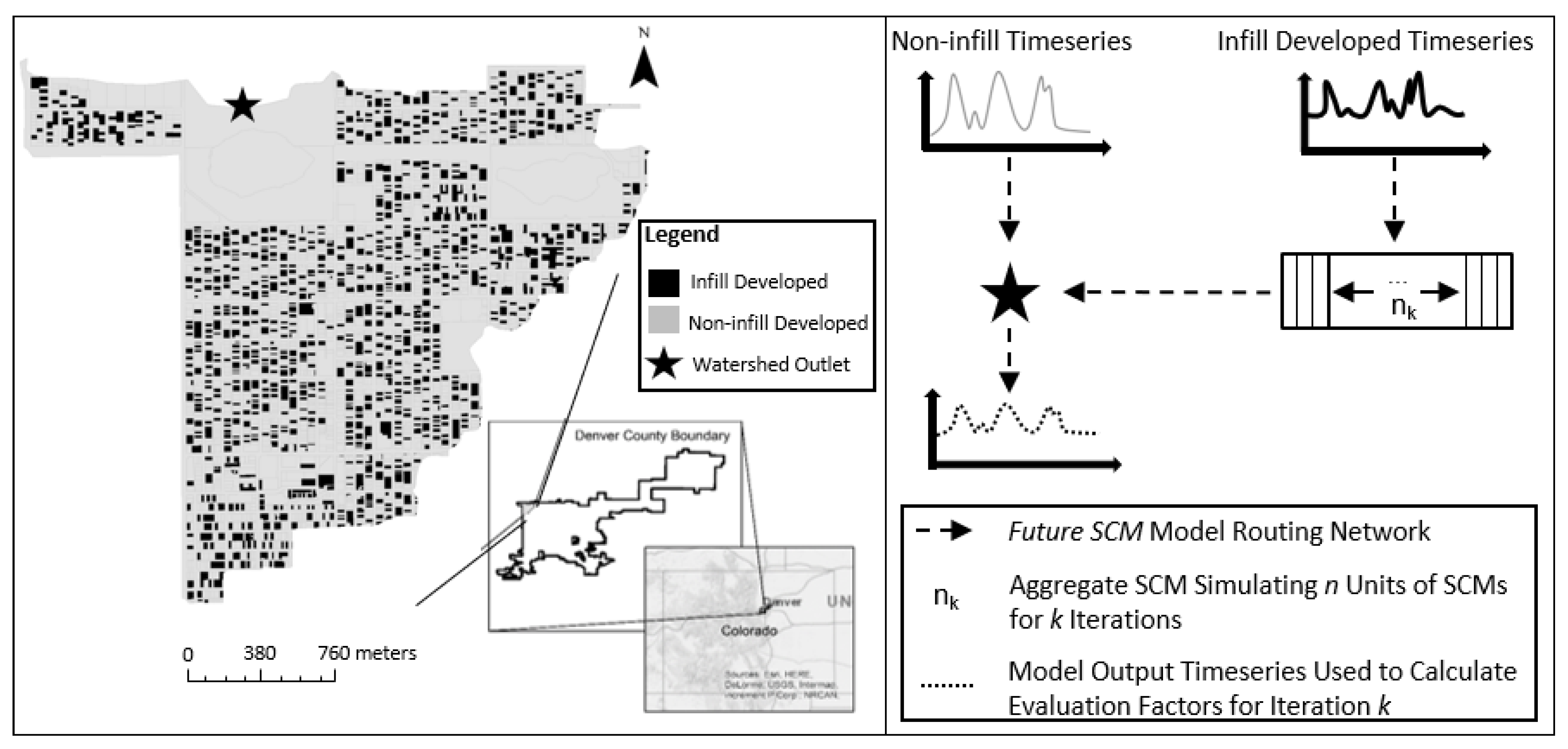
2. Study Area
3. Methods
3.1. Model
3.1.1. Water Quantity Data
3.1.2. Water Quality Data
3.1.3. Modeled SCMs
3.1.4. Model Routing
3.2. Model Validation
3.3. Optimization Scenarios
- set of SCM solutions associated with location i
- = computed amount of water quantity factor at assessment point j
- = the maximum value of the water quantity factor targeted at assessment point j
- = computed amount of water quality factor at assessment point k
- = the maximum value of the water quality factor targeted at assessment point k
- = the management evaluation factor (EF) at one given assessment point, and the EF can be any of the options listed in Table 2
3.3.1. Individual Optimization
3.3.2. Full Optimization
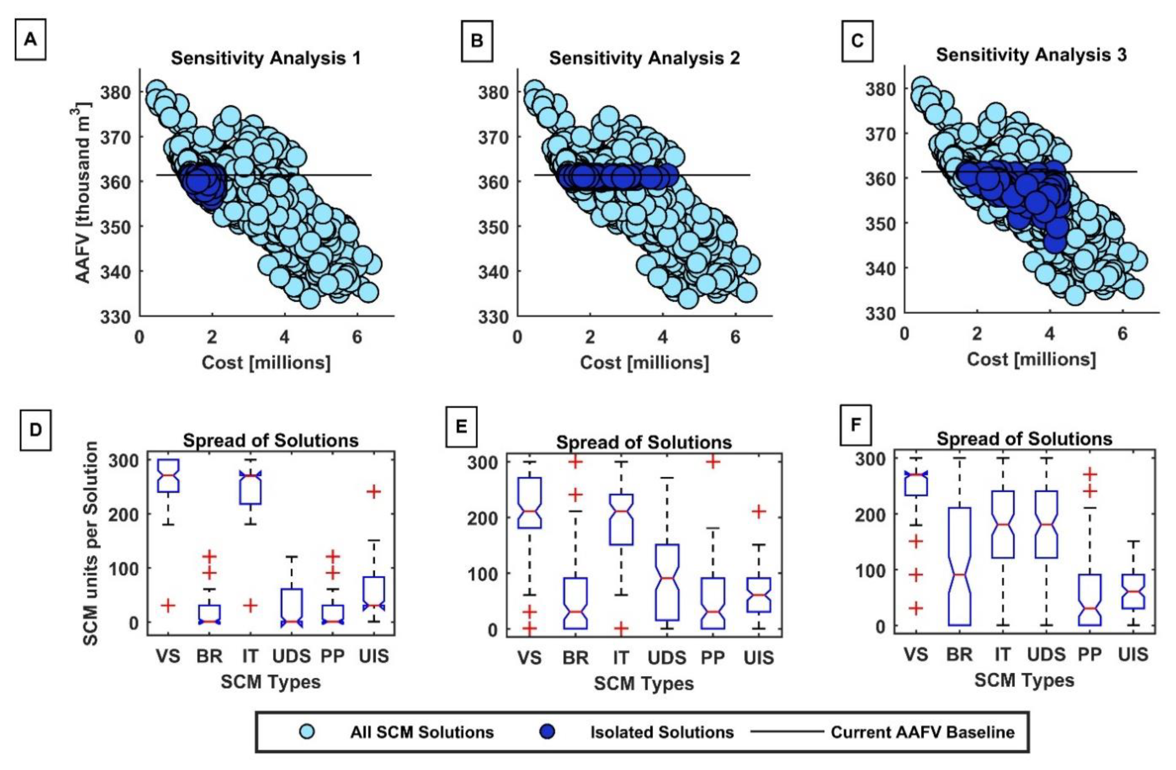
3.3.3. Full Optimization Selection Criteria Sensitivity Analysis
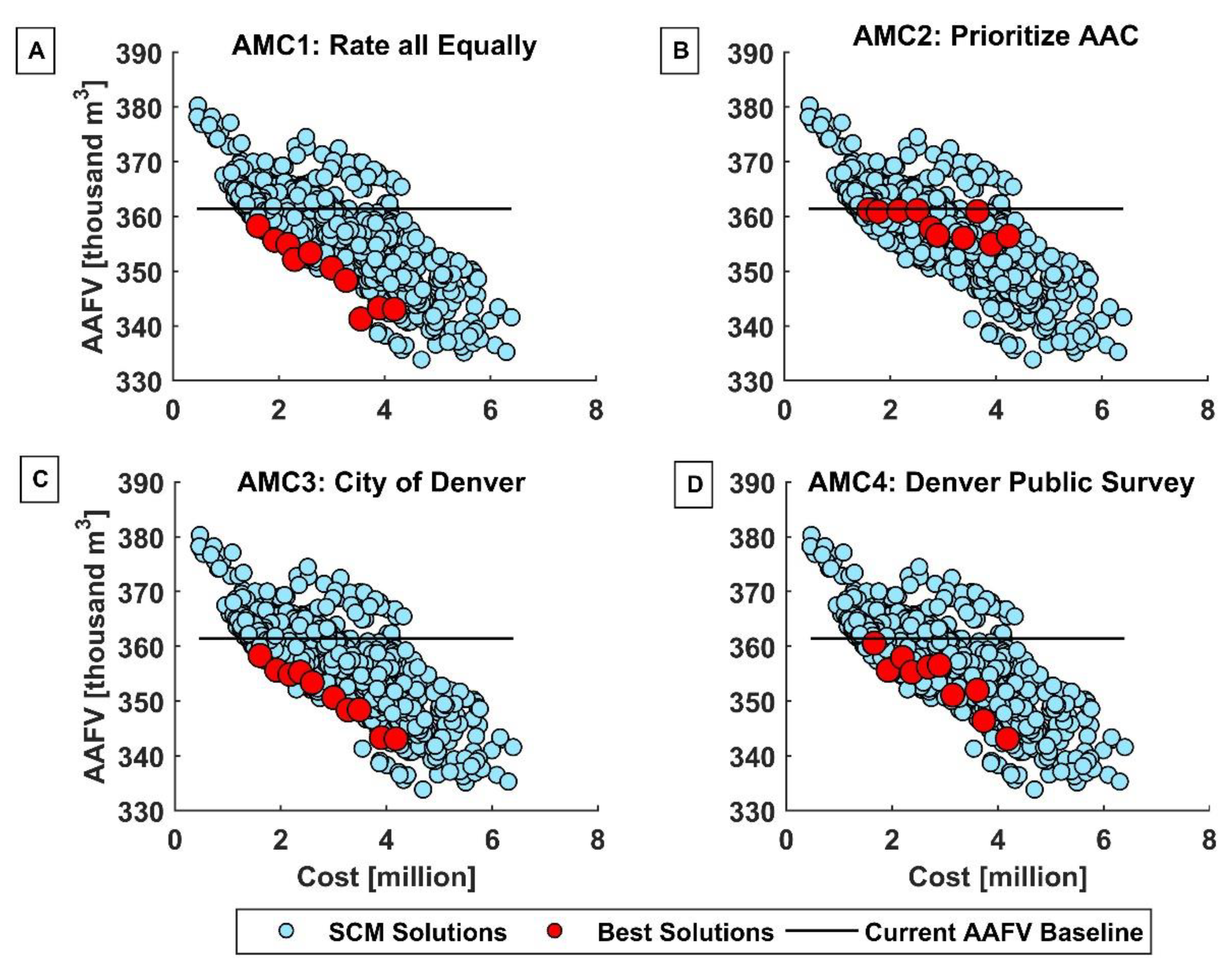
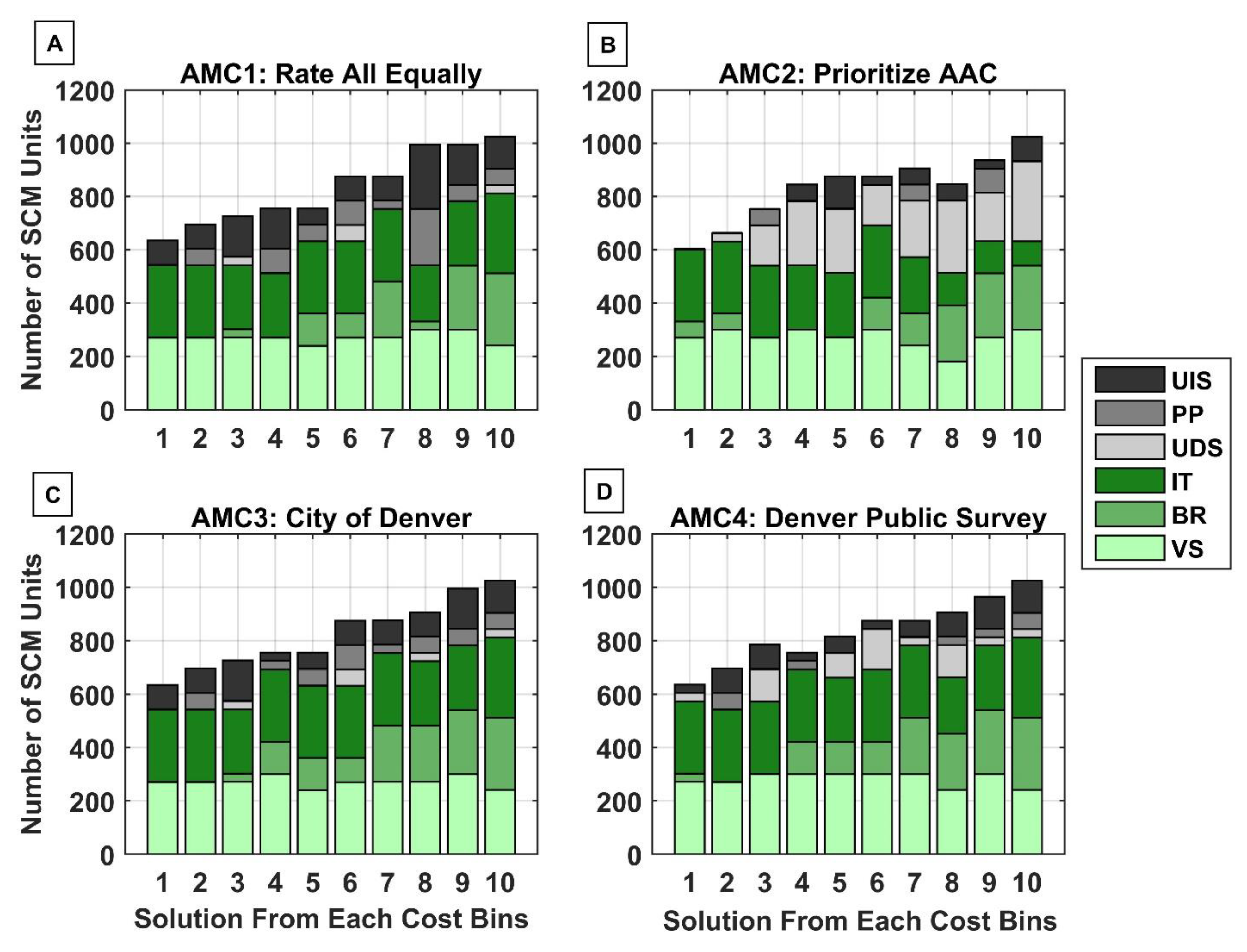
3.3.4. Full Optimization Aggregate Multi-Criteria (AMC) Selection
4. Results
4.1. Model Validation Results
4.2. Individual Optimization Results
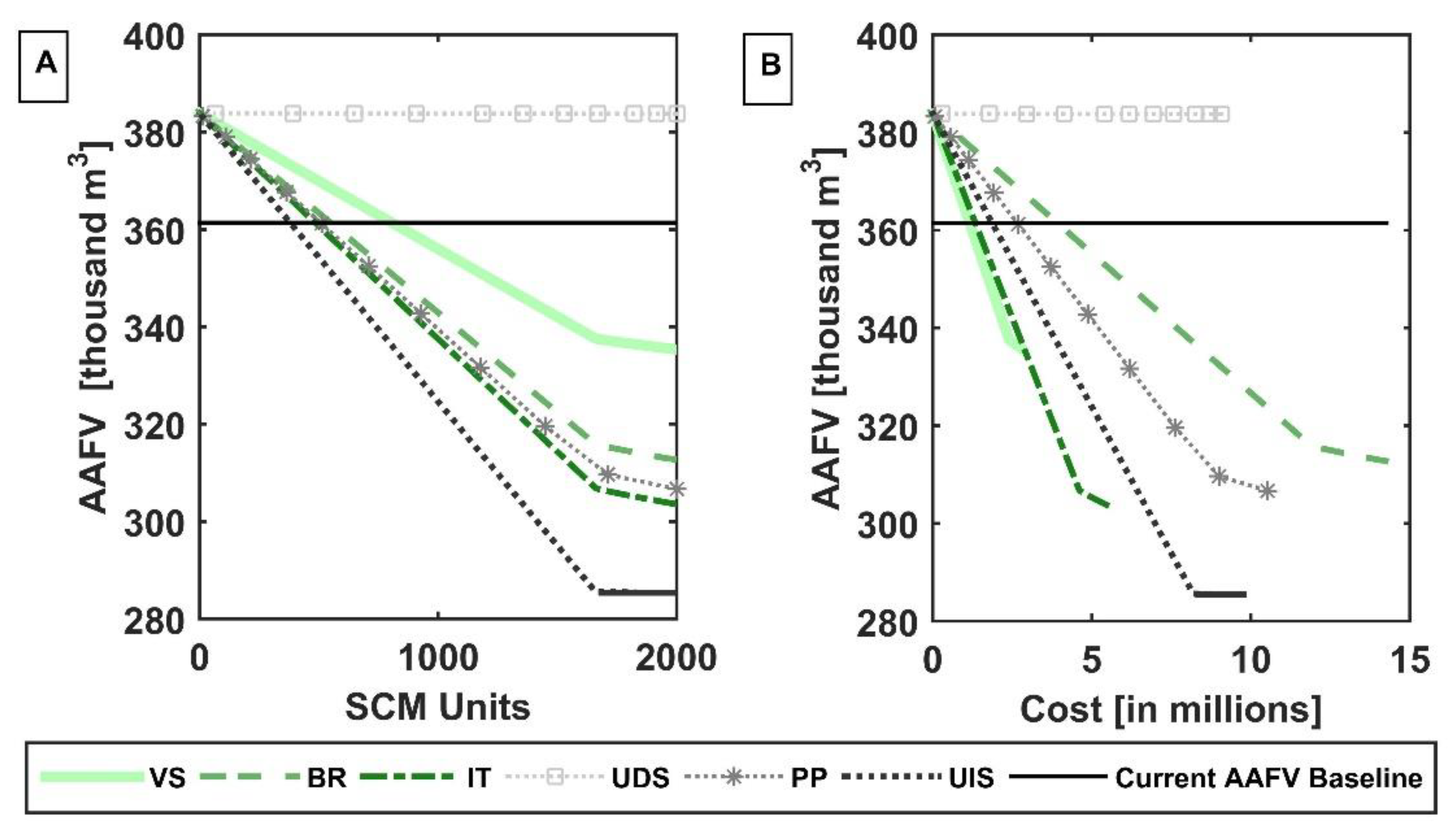
4.2.1. Water Quantity Results
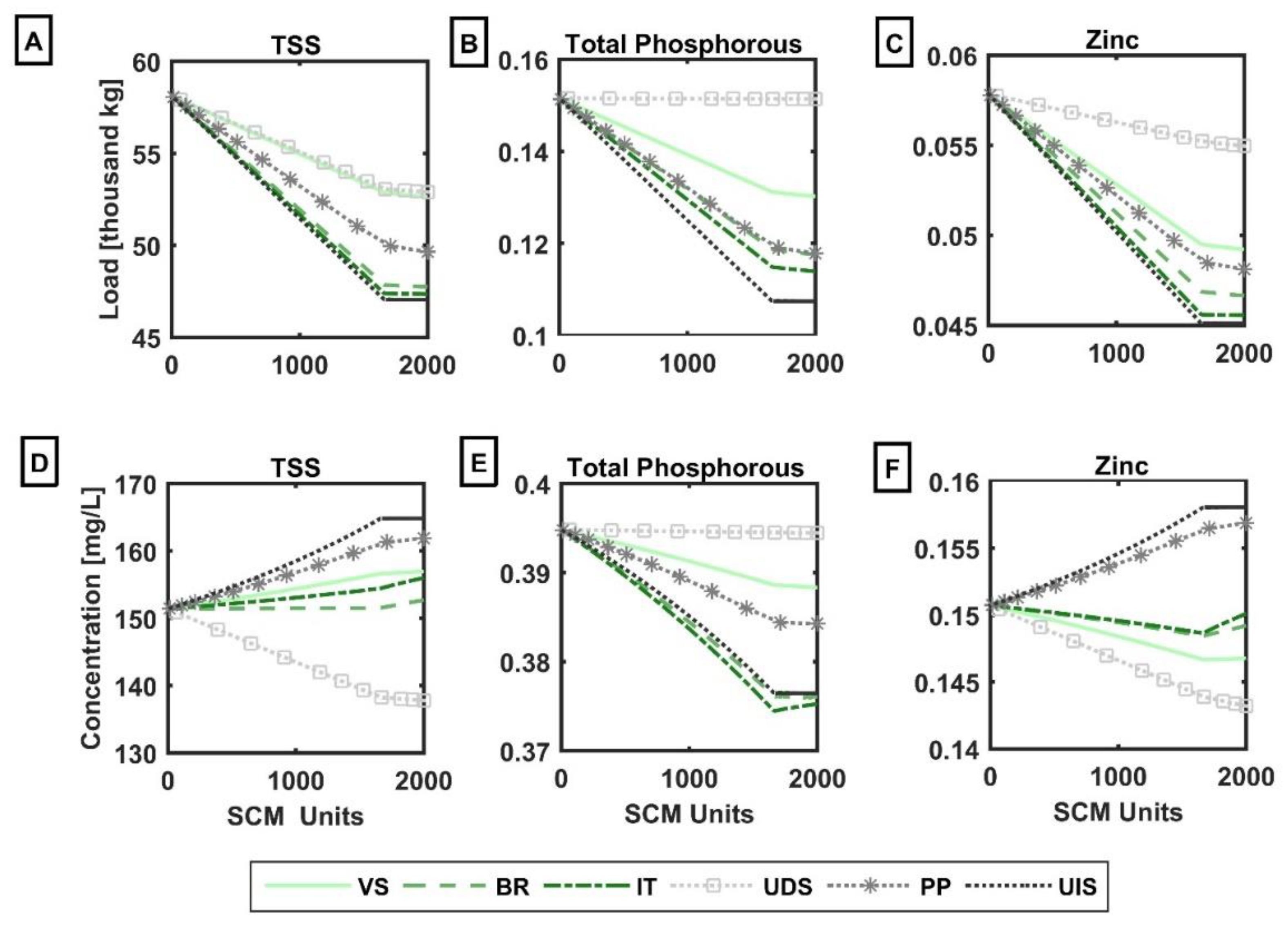
4.2.2. Water Quality Results
4.2.3. AAFV Criteria Solution Selection Results
4.3. Full Optimization Results
4.3.1. Selection Criteria Sensitivity Analysis Results
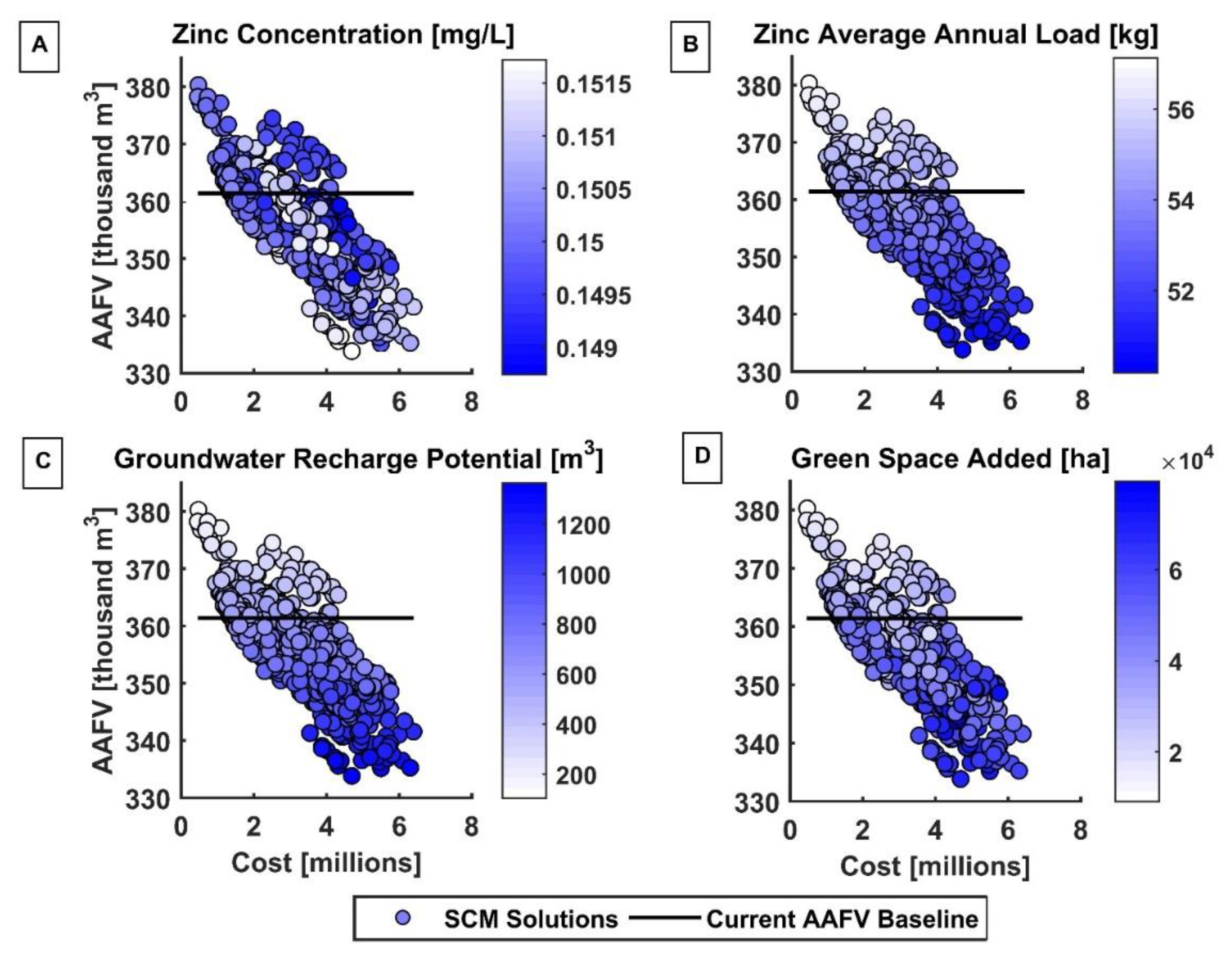
4.3.2. Aggregate Multi-Criteria Results
5. Discussion
5.1. Benefits and Tradeoffs of Green to Grey Infrastructure
5.1.1. Hydrologic Performance
5.1.2. Cost
5.1.3. Added Greenness
5.2. Impact of Decision Maker Priorities on Planning-Level Decisions
6. Conclusions
Author Contributions
Funding
Acknowledgments
Conflicts of Interest
Appendix A
- Algorithms: Scatter search and NSGAII determine how the optimization module creates a population of solutions and how that population evolves over time based on the optimal solutions (determined by the controls). While scatter search uses a clumping of the best solutions, NSGAII uses the single best solution along the Pareto frontier.
- Controls: Cost minimization and a cost effectiveness curve determine how the optimization module determines the optimal solutions. Cost minimization aims to minimize cost while achieving a certain evaluation factor goal. A cost effectiveness curve aims to both minimize cost and maximize an evaluation curve within a target range simultaneously.
- Number of SCM units: This sets the lower and higher bounds of the number of SCM units the model can simulate in each solution. Users can set these bounds to be wide so that the model looks at only implementing one SCM unit all the way to enough SCM units to capture water from the whole watershed. The user can also set a stricter bound if they know a general range of SCMs that will reach a desired goal.
- Step of SCM unit: This sets the step at which the optimization module may select SCM units. For example, if the user sets a step of five, the model will only simulate 5, 10, 15, etc. units of a certain SCM type.
- Target evaluation range: The target evaluation range is what tells the optimization module where to look for the optimal solutions. Cost minimization only uses one target evaluation number. The model looks for the best solutions that reach this goal at a minimum cost. The cost evaluation control uses two evaluation targets. The optimization module looks for the optimal solutions within that range.
References
- Booth, D.B.; Bledsoe, B.P. Streams and Urbanization. In The Water Environment of Cities; Baker, L.A., Ed.; Springer: New York, NY, USA, 2009; pp. 93–123. [Google Scholar] [CrossRef]
- Brabec, E.; Schulte, S.; Richards, P.L. Impervious Surfaces and Water Quality: A Review of Current Literature and Its Implications for Watershed Planning. J. Plan. Lit. 2002, 16, 499–514. [Google Scholar] [CrossRef]
- Paul, M.J.; Meyer, J.L. Streams in the Urban Landscape. Annu. Rev. Ecol. Syst. 2001, 32, 333–365. [Google Scholar] [CrossRef]
- Driscoll, M.O.; Clinton, S.; Jefferson, A.; Manda, A.; Mcmillan, S. Urbanization Effects on Watershed Hydrology and In-Stream Processes in the Southern United States. Water 2010, 2, 605–648. [Google Scholar] [CrossRef]
- USEPA. National Summary of State Information: Assessed Waters of United States. Available online: https://ofmpub.epa.gov/waters10/attains_nation_cy.control (accessed on 1 January 2018).
- NRC. Urban Stormwater Management in the United States; National Research Council: Washington, DC, USA, 2008. [Google Scholar]
- USEPA. Preliminary Data Summary of Urban Storm Water Best Management Practices (No. EPA-821-R-99-012); USEPA: Washington, DC, USA, 1999.
- Liu, Y.; Engel, B.A.; Flanagan, D.C.; Gitau, M.W.; Mcmillan, S.K.; Chaubey, I. A Review on Effectiveness of Best Management Practices in Improving Hydrology and Water Quality: Needs and Opportunities. Sci. Total Environ. 2017, 601–602, 580–593. [Google Scholar] [CrossRef]
- UDFCD. Urban Storm Drainage Criteria Manual: Volume 3 Best Management Practices; UDFCD: Denver, CO, USA, 2010.
- Bracmort, K.S.; Arabi, M.; Frankenberger, J.R.; Engel, B.A.; Arnold, J.G. Modeling Long-Term Water Quality Impact of Structural BMPs. Am. Soc. Agric. Biol. Eng. 2006, 49, 367–374. [Google Scholar] [CrossRef]
- Ando, A.W.; Netusil, N.R. Valuing the Benefits of Green Stormwater Infrastructure. Oxf. Res. Encycl. Environ. Sci. 2018, 1–26. [Google Scholar] [CrossRef]
- Charlesworth, S.M.; Booth, C.A. (Eds.) Sustainable Surface Water Management: A Handbook for SuDS; Wiley: Hoboken, NJ, USA, 2016. [Google Scholar] [CrossRef]
- Clean Water Act. EPA Administered Permit Programs: The Natinoal Pollutant Discharge Elimination System; USEPA: Washington, DC, USA, 2011; Volume 40 CFR Par.
- Spahr, K. Contextualizing and Communicating the Ancillary Benefits of Green Stormwater Infrastructure; Colorado School of Mines: Golden, CO, USA, 2020. [Google Scholar]
- Brown, R.R. Local Institutional Development and Organizational Change for Advancing Sustainable Urban Water Futures. J. Environ. Plan. Manag. 2008, 41, 221–233. [Google Scholar] [CrossRef]
- Fitzgerald, J.; Laufer, J. Governing Green Stormwater Infrastructure: The Philadelphia Experience. Local Environ. 2017, 22, 256–268. [Google Scholar] [CrossRef]
- Roesner, L.A.; Bledsoe, B.P.; Brashear, R.W. Are Best-Management-Practice Criteria Really Environmentally Friendly? J. Water Resour. Plan. Manag. 2001, 127, 150–154. [Google Scholar] [CrossRef]
- Sun, Y.; Li, Q.; Liu, L.; Xu, C.; Liu, Z. Hydrological Simulation Approaches for BMPs and LID Practices in Highly Urbanized Area and Development of Hydrological Performance Indicator System. Water Sci. Eng. 2014, 7, 143–154. [Google Scholar] [CrossRef]
- Karr, J.R.; Dudley, D.R. Ecological Perspective on Water Quality Goals. J. Environ. Manag. 1981, 5, 55–68. [Google Scholar] [CrossRef]
- Bell, C.D.; Spahr, K.; Grubert, E.; Stokes-draut, J.; Gallo, E.; Mccray, J.E.; Hogue, T.S. Decision Making on the Gray-Green Stormwater Infrastructure Continuum. J. Sustain. Water Built. Environ. 2019, 5. [Google Scholar] [CrossRef]
- CMWR. Tunnel and Reservoir Plan (TARP) Fact Sheet; Chicago Metropolitan Water Reclamation: Chicago, IL, USA, 2013.
- LADPH. Guidelines for Alternate Water Sources: Indoor and Outdoor Non-Potable Uses; Los Angeles County Department of Public Health: Los Angeles, CA, USA, 2016.
- USEPA. Storm Water Technology Fact Sheet: On-Site Underground Retention/detention; USEPA: Washington, DC, USA, 2001.
- NYCDEP. Guidelines for the Design and Construction of Stormwater Management Systems; New York City Department of Environmental Protection: New York, NY, USA, 2012.
- Contech. Underground Stormwater Detention & Infiltration; Contech Engineered Solutions LLC: West Chester, OH, USA, 2019. [Google Scholar]
- International Stormwater BMP Database. Available online: http://www.bmpdatabase.org/ (accessed on 1 January 2016).
- Cessna, J. Underground Stormwater Storage Case Studies. Stormwater. 2017. Available online: https://www.stormh2o.com/bmps/article/13030318/underground-stormwater-storage-case-studies (accessed on 25 May 2020).
- New York State. Stormwater Management Design Manual Chapter 10: Enhanced Phosphorus Removal Supplement; New York State: New York, NY, USA, 2015.
- Mcintosh, N.; Drake, J.; Young, D.; Spencer, J. Modeling Sedimentation in Underground Stormwater Detention Chamber Systems. In International Low Impact Development Conference 2015: It Works in All Climates and Soils; Asce Library: Houston, TX, USA, 2015; pp. 43–52. [Google Scholar]
- Smart, P. Modeling Underground Stormwater Storage; HydroCAD Software Solutions: Tamworth, NH, USA, 2020. [Google Scholar]
- Zawiliski, X.; Sakson, X. Modelling of Detention-Sedimentation Basins for Stormwater Treatment Using SWMM Software. In Proceedings of the 11th International Conference on Urban Drainage, Edinburgh, UK, 31 August–5 September 2008; pp. 1–10. [Google Scholar]
- Jayanti, S.; Narayanan, S. Computational Study of Particle-Eddy Interaction in Sedimentation Tanks. J. Environ. Eng. 2004, 130, 37–49. [Google Scholar] [CrossRef]
- Martino, G.D.; Paolo, F.D.; Fontana, N.; Marini, G.; Ranucci, A. Pollution Reduction in Receivers: Storm-Water Tanks. J. Urban Plan. Dev. 2011, 137, 29–38. [Google Scholar] [CrossRef]
- Wang, G.; Chen, S.; Barber, M.E.; Yonge, D.R. Modeling Flow and Pollutant Removal of Wet Detention Pond Treating Stormwater Runoff. J. Environ. Eng. 2004, 130, 1315–1321. [Google Scholar] [CrossRef]
- Jefferson, A.J.; Hopkins, K.G.; Fanelli, R.; Avellaneda, P.M.; Mcmillan, S.K. Stormwater Management Network Effectiveness and Implications for Urban Watershed Function: A Critical Review. Hydrol. Process. 2017, 31, 4056–4080. [Google Scholar] [CrossRef]
- Golden, H.E.; Hoghooghi, N. Green Infrastructure and Its Catchment-Scale Effects: An Emerging Science. Wiley Interdiscip. Rev. Water 2018, 5, e1254. [Google Scholar] [CrossRef]
- Gallo, E.; Bell, C.D.; Mika, K.; Gold, M.; Hogue, T.S. Stormwater Management Options and Decision-Making in Urbanized Watersheds of Los Angeles, California. J. Sustain. Water Built. Environ. 2020, 6, 1–14. [Google Scholar] [CrossRef]
- Wolfand, J.M.; Bell, C.D.; Boehm, A.B.; Hogue, T.S.; Luthy, R.G. Multiple Pathways to Bacterial Load Reduction by Stormwater Best Management Practices: Trade-Offs in Performance, Volume, and Treated Area. Environ. Sci. Technol. 2018, 52, 6370–6379. [Google Scholar] [CrossRef]
- Nolan, T.N.; Goodstein, L.D.; Goodstein, J. Chapter 1—Introduction to Applied Strategic Planning. In Applied Strategic Planning; Pfeiffer: San Francisco, CA, USA, 2008; pp. 1–10. [Google Scholar]
- Downs, B. The Strategic Planning Process in Six Steps. Available online: https://www.bbgbroker.com/strategic-planning-process-6-steps/ (accessed on 25 May 2020).
- Shoemaker, L.; Riverson, J.; Alvi, K.; Zhen, J.; Paul, S.; Rafi, T. SUSTAIN User’s Manual—A Framework for Placement of Best Management Practices in Urban Watersheds to Protect Water Quality; USEPA: Washington, DC, USA, 2009.
- Limbrunner, J.F.; Vogel, R.M.; Chapra, S.C.; Kirchen, P.H. Classic Optimization Techniques Applied to Stormwater and Nonpoint Source Classic Optimization Techniques Applied to Stormwater and Nonpoint Source Pollution Management at the Watershed Scale. J. Water Resour. Plan. Manag. 2013, 139. [Google Scholar] [CrossRef]
- Hipp, J.A.; Lejano, R.; Smith, C.S. Optimization of Stormwater Filtration at the Urban/Watershed Interface. Environ. Sci. Technol. 2006, 40, 4794–4801. [Google Scholar] [CrossRef] [PubMed]
- Perez-pedini, C.; Limbrunner, J.F.; Vogel, R.M. Optimal Location of Infiltration-Based Best Management Practices for Storm Water Management. J. Water Resour. Plan. Manag. 2006, 131, 441–448. [Google Scholar] [CrossRef]
- Zhang, G.; Hamlett, J.M.; Reed, P.; Tang, Y. Multi-Objective Optimization of Low Impact Development Scenarios in an Urbanizing Watershed. Open J. Optim. 2012, 2, 95–108. [Google Scholar] [CrossRef]
- Baek, S.; Choi, D.; Jung, J.; Lee, H.; Lee, H.; Yoon, K.; Hwa, K. Optimizing Low Impact Development (LID) for Stormwater Runoff Treatment in Urban Area, Korea: Experimental and Modeling Approach. Water Res. 2015, 86, 122–131. [Google Scholar] [CrossRef] [PubMed]
- Yang, Y.; Fong, T.; Chui, M. Optimizing Surface and Contributing Areas of Bioretention Cells for Stormwater Runoff Quality and Quantity Management. J. Environ. Manag. 2018, 206, 1090–1103. [Google Scholar] [CrossRef]
- Jenq, T.; Uchrin, C.G.; Granstrom, M.L.; Hsueh, S. A Linear Program Model for Point-Nonpoint Source Control Decisions: Theoretical Development. Ecol. Modell. 1983, 19, 249–262. [Google Scholar] [CrossRef]
- Schleich, J.; White, D. Cost Minimization of Nutrient Reduction in Watershed Managemetn Using Linear Programming. J. Am. Water Resour. Assoc. 1997, 33, 135–142. [Google Scholar] [CrossRef]
- Loáiciga, H.A.; Sadeghi, K.M.; Shivers, S.; Kharaghani, S. Stormwater Control Measures: Optimization Methods for Sizing and Selection. J. Water Resour. Plan. Manag. 2015, 141, 1–10. [Google Scholar] [CrossRef]
- Mays, L.W.; Bedient, P.B. Model for Optimal Size and Location of Detention. J. Water Resour. Plan. Manag. 1982, 108, 270–285. [Google Scholar]
- Sample, D.J.; Heaney, J.P.; Wright, L.T.; Koustas, R. Geographic Information Systems, Decision Support Systems, and Urban Storm-Water Management. J. Water Resour. Plan. Manag. 2001, 127, 155–161. [Google Scholar] [CrossRef]
- Panos, C.L.; Hogue, T.S.; Gilliom, R.L.; Mccray, J.E. High-Resolution Modeling of Infill Development Impact on Stormwater Dynamics in Denver, Colorado. J. Sustain. Water Built. Environ. 2018, 4, 1–14. [Google Scholar] [CrossRef]
- Thomas, J.V. Residential Construction Trends in America’s Metropolitan Regions; U.S. Environmental Protection Agency: Development, Community, and Environment Division: Washington, DC, USA, 2009.
- USEPA. Summary of State Post Construction Stormwater Standards; EPA: Office of Water, Office of Wastewater Management, Water Permits Division: Washington, DC, USA, 2016.
- Cherry, L.; Mollendor, D.; Eisenstein, B.; Hogue, T.S.; Peterman, K.; Mccray, J.E. Predicting Parcel-Scale Redevelopment Using Linear and Logistic Regression—The Berkeley Neighborhood Denver, Colorado Case Study. Sustainability 2019, 11, 1882. [Google Scholar] [CrossRef]
- City and County of Denver. Storm Drainage Design & Technical Criteria; City and County of Denver: Denver, CO, USA, 2013.
- City and County of Denver. Storm Drainage Master Plan; City and County of Denver: Denver, CO, USA, 2019.
- City and County of Denver Public Works. Green Infrastructure Implementation Strategy; City and County of Denver Public Works: Denver, CO, USA, 2018.
- LADPW. Stormwater Best Management Practice Design and Maintenance Manual For Publicly Maintained Storm Drain Systems; County of Los Angeles Department of Public Works: Los Angeles, CA, USA, 2010.
- Minneapolis Public Works. Stormwater and Sanitary Sewer Guide; Minneapolis Public Works: Minneapolis, MN, USA, 2017.
- State of Michigan. Rogue River Outfall Disinfection Project; State of Michigan: Lansing, MI, USA, 2017; Volume 7.
- IDEQ. Idaho Catalog of Stormwater Best Management Practices; Idaho Department of Environmental Quality: Boise, ID, USA, 2020.
- Panos, C.L.; Wolfand, J.M.; Hogue, T.S. SWMM Sensitivity to LID Siting and Routing Parameters: Implications for Stormwater Regulatory Compliance. J. Am. Water Resour. Assoc. 2020, 1–20. [Google Scholar] [CrossRef]
- Bell, C.D.; Wolfand, J.; Hogue, T.S. Regionalization of Default Parameters for Urban Stormwater Quality Models. J. Am. Water Resour. Assoc. 2019. in review. [Google Scholar]
- City and County of Denver. Ultra-Urban Green Infrastructure Guidelines; City and County of Denver: Denver, CO, USA, 2016.
- StormTrap. Capital Cost Budget Estimates for Detention/Infiltration Systems; StormTrap: Romeoville, IL, USA, 2018. [Google Scholar]
- RSMeans. Masterformat City Cost Indexes: Year 2019 Base; RSMeans: Everett, WA, USA, 2019. [Google Scholar]
- Urbonas, B.; Guo, J.C.Y.; Tucker, L.S. Sizing Capture Volume for Stormwater Quality Enhancement; Urban Drainage and Flood Control District: Denver, CO, USA, 1989.
- Clapp, R.B.; Hornberger, G.M. Empirical Equations for Some Soil Hydraulic Properties. Water Resour. Res. 1978, 14, 601–604. [Google Scholar] [CrossRef]
- Minnesota Stormwater Design Team. Minnesota Stormwater Manual; Pollution Control Agency: Glencoe, MN, USA, 2013.
- Panos, C. Advancing Understanding and Prediction of Redevelopment Impacts on Stormwater Runoff in Semi-Arid Urban Areas; Colorado School of Mines: Golden, CO, USA, 2020. [Google Scholar]
- USGS. StreamStats Report: Basin Characteristics for Berkeley Neighborhood; USGS: Denver, CO, USA, 2017.
- Branke, J.; Deb, K.; Dierolf, H.; Osswald, M. Finding Knees in Multi-Objective Optimization. In Parrallel Problem Solving from Nature; Springer: New York, NY, USA, 2004; pp. 722–731. [Google Scholar]
- Samuelson, P.A. The Pure Theory of Public Expenditure. Rev. Econ. Stat. 1954, 387–389. [Google Scholar] [CrossRef]
- Plantinga, A.J.; Wu, J. Co-Benefits from Carbon Sequestration in Forests: Evaluating Reductions in Agricultural Externalities from an Afforestation Policy in Wisconsin. Land Econ. 2003, 79, 74–85. [Google Scholar] [CrossRef]
- Mcauley, A.; Knights, D. What Should It Cost to Maintain Stormwater Treatment Systems? A Case Study from ACT. In Proceedings of the 9th International Water Sensitive Urban Design (WSUD 2015), Sydney, Australia, 19–23 October 2015; pp. 340–350. [Google Scholar]
- Liao, Z.; Chen, H.; Huang, F.; Li, H. Cost–effectiveness Analysis on LID Measures of a Highly Urbanized Area. Desalin. Water Treat. 2014, 56, 2817–2823. [Google Scholar] [CrossRef]
- Rebitzer, G.; Hunkeler, D.; Jolliep, O. LCC-The Economic Pillar of Sustainability: Methodology and Application to Watewater Treatment. Environ. Prog. 2003, 22, 241–249. [Google Scholar] [CrossRef]
- Panagopoulos, Y.; Makropoulos, C.; Mimikou, M. Reducing Surface Water Pollution through the Assessment of the Cost-Effectiveness of BMPs at Different Spatial Scales. J. Environ. Manag. 2011, 92, 2823–2835. [Google Scholar] [CrossRef]
- Jaffe, M. Reflections on Green Infrastructure Economics. Environ. Pract. 2010, 12, 390–395. [Google Scholar] [CrossRef]
- McGarity, A.; Hung, F.; Rosan, C.; Hobbs, B.; Heckert, M.; Szalay, S. Quantifying Benefits of Green Stormwater Infrastructure in Philadelphia. In World Environmental and Water Resources Congress; ASCE: Raston, VA, USA, 2015; pp. 409–420. [Google Scholar]
- Cadavid, L.C.; Ando, A.W. Valuing Preferences over Stormwater Management Outcomes Including Improved Hydrologic Function. Water Resour. Res. 2013, 49, 4114–4125. [Google Scholar] [CrossRef]
- Alves, A.; Vojinovic, Z.; Kapelan, Z.; Sanchez, A.; Gersonius, B. Exploring Trade-Offs among the Multiple Benefits of Green-Blue-Grey Infrastructure for Urban Flood Mitigation. Sci. Total Environ. 2020, 703, 134980. [Google Scholar] [CrossRef] [PubMed]


| Current Baseline (No Infill Development) (ha) | % of Total | Future Baseline (Non-Infill Developed Area) (ha) | % of Total | Future Baseline (Infill Developed Area) (ha) | % of Total | |
|---|---|---|---|---|---|---|
| Commercial | 18 | 3.81 | 18 | 4.68 | 0.00 | 0.00 |
| Industrial | 13 | 2.68 | 13 | 3.30 | 0.00 | 0.00 |
| Residential | 222 | 46.72 | 134 | 34.69 | 89 | 100.00 |
| Transportation | 134 | 28.15 | 134 | 34.60 | 0.00 | 0.00 |
| Parks | 65 | 13.63 | 64 | 16.56 | 0.00 | 0.00 |
| Surface Water | 24 | 5.02 | 24 | 6.17 | 0.00 | 0.00 |
| Total Area | 475 | 100.00 | 387 | 100.00 | 89 | 100.00 |
| SCM Types | Evaluation Factors |
|---|---|
| Green roof | Annual and seasonal * average flow volume |
| Bioretention | Flow exceedance frequency |
| Infiltration trench | Flow duration curve |
| Vegetated swale | Peak discharge flow |
| Dry pond | Annual and seasonal groundwater recharge potential * |
| Wet pond | Annual and seasonal average evapotranspiration * |
| Buffer strip | Annual and seasonal * average loads |
| Porous pavement | Annual and seasonal * average concentration |
| Rain barrel | Days above concentration threshold |
| Underground detention structure * | |
| Underground infiltration structure * | |
| Underground gravel bed * | |
| Aboveground gravel bed * |
| Pollutant EMCs (mg/L) | Mean | Min | 25th | Median | 75th | Max |
|---|---|---|---|---|---|---|
| TSS | ||||||
| Commercial | 210.33 | 1.00 | 37.83 | 118.00 | 275.27 | 1940.00 |
| Paved area | 125.92 | 0.50 | 33.08 | 68.00 | 130.00 | 4800.00 |
| Industrial | 507.04 | 16.00 | 186.00 | 370.00 | 773.00 | 2325.00 |
| Open park space | 602.07 | 194.05 | 293.57 | 516.00 | 845.94 | 1400.00 |
| Residential | 201.76 | 0.30 | 49.00 | 112.50 | 247.49 | 2732.43 |
| TP | ||||||
| Commercial | 0.40 | 0.008 | 0.14 | 0.26 | 0.48 | 6.30 |
| Paved area | 0.39 | 0.070 | 0.15 | 0.28 | 0.42 | 2.60 |
| Industrial | 0.94 | 0.030 | 0.27 | 0.72 | 1.30 | 7.90 |
| Open park space | 0.52 | 0.210 | 0.33 | 0.53 | 0.64 | 1.00 |
| Residential | 0.56 | 0.03 | 0.29 | 0.45 | 0.71 | 4.96 |
| Zn | ||||||
| Commercial | 0.34 | 0.015 | 0.16 | 0.26 | 0.40 | 3.61 |
| Paved area | 0.24 | 0.001 | 0.08 | 0.16 | 0.28 | 2.10 |
| Industrial | 0.54 | 0.005 | 0.31 | 0.47 | 0.69 | 2.40 |
| Open park space | 0.26 | 0.040 | 0.09 | 0.20 | 0.35 | 0.73 |
| Residential | 0.16 | 0.0025 | 0.07 | 0.13 | 0.20 | 1.50 |
| EMCs (mg/L) | Current Baseline (No Infill Development) | Future Baseline (Non-Infill Developed Area) | Future Baseline (Infill Developed Area) |
|---|---|---|---|
| TSS | 157.46 | 164.82 | 112.47 |
| TP | 0.39 | 0.38 | 0.45 |
| Zn | 0.15 | 0.16 | 0.13 |
| Parameter | VS | BR | IT | UDS | PP | UIS |
|---|---|---|---|---|---|---|
| Capital cost (per m3) | 281.50 I | 408.23 I | 168.80 I | 493.69 J | 438.61 I | 424.13 J |
| Surface storage layer | ||||||
| Width (m) | 0.30 A | 1.52 B | 1.52 B | 2.52 F | 1.52 B | 2.31 F |
| Length (m) | 11.06 A | 12.19 B | 12.17 B | 2.52 F | 12.17 B | 2.31 F |
| Surface area (m2) | 16.86 | 18.54 | 18.54 | 6.35 | 18.54 | 5.35 |
| Green space added (m2) | 16.86 | 18.54 | 18.54 | 0 | 0 | 0 |
| Slope A | 5.5% | - | -- | - | - | |
| Weir height (m) | 0.15 A | 0.15 B | 0.23 B | 1.45 C | 0.01 B | 1.45 C |
| Weir width (m) | - | 0.30 | 0.30 | NA | 1.52 | NA |
| Vegetative fraction E | 0.2 | 0.2 | 0.2 | 0.2 | 0.2 | 0.2 |
| Orifice height (m) | - | 0.01 | - | 0.03 | - | - |
| Orifice diameter (cm) A | - | 0.39 | - | 0.39 | - | - |
| Soil storage layer | ||||||
| Infiltration method | Green Ampt | Green Ampt | Green Ampt | Green Ampt | Green Ampt | Green Ampt |
| Soil depth (m) B, F | 0.15 | 0.79 | 0.65 | - | 0.65 | 0.65 |
| Porosity D | 0.42 | 0.435 | 0.41 | - | 0.435 | 0.41 |
| Field capacity E | 0.1 | 0.1 | 0.1 | 0.1 | 0.1 | 0.1 |
| Wilting point E | 0.095 | 0.095 | 0.095 | 0.095 | 0.095 | 0.095 |
| Soil types | Sandy clay loam | Sandy loam | Loamy sand | - | Sandy loam | Loamy sand |
| Soil layer infiltration (cm/hour) A | 0.13 | 0.25 | 0.55 | 0 | 0.25 | 0.55 |
| Suction head (m) E | 0.91 | 0.91 | 0.91 | 0 | 0.91 | 0.91 |
| Underdrain storage layer | ||||||
| Consider underdrain? | no | yes | yes | no | yes | no |
| Void ratio E | - | 0.3 | 0.3 | - | 0.3 | - |
| Back infill rate (cm/hour) G | - | 0.08 | 0.08 | - | 0.08 | - |
| Media below drain (m) B | - | 0.03 | 0.15 | - | 0.08 | - |
| Pollutant decay rates | ||||||
| IBMPD data source H | CA RVTS System | Lakewood CO Iris Garden | Lakewood CO Dry Pond | Lakewood CO Retention Vault | NA | Lakewood CO Retention Vault |
| TSS (1/year) | 0.122 | 2.15 | 0.757 | 0.396 | 0.00 | 0.396 |
| TP (1/year) | 0.00 | 0.0997 | 0.059 | 0.00015 | 0.00 | 0.00015 |
| Zn (1/year) | 4.864 | 0.72 | 0.615 | 0.038 | 0.00 | 0.038 |
| Benefit Ratings | AMC1 (Equal) | AMC2 (Prioritize AAC) | AMC3 (City of Denver) | AMC4 (Public Survey) |
|---|---|---|---|---|
| AAFV | 5 | 0 | 4 | 3 |
| Zn AAC | 5 | 5 | 4 | 5 |
| Zn AAL | 5 | 0 | 5 | 3 |
| GWRP | 5 | 0 | 0 | 2 |
| Green Space Added | 5 | 0 | 4 | 1 |
| Current Baseline | Future Baseline | Future BR 1% Sizing | Future BR 5% Sizing | |
|---|---|---|---|---|
| 2-year storm | ||||
| NSE | 1 | 1 | 0.991 | 0.844 |
| R2 | 1 | 1 | 0.996 | 0.996 |
| % Bias | −0.007 | −0.0008 | −1.710 | 1.920 |
| 5-year storm | ||||
| NSE | 1 | 1 | 0.995 | 0.933 |
| R2 | 1 | 1 | 0.997 | 0.997 |
| % Bias | −0.007 | −0.0008 | −1.953 | −6.276 |
| 10-year storm | ||||
| NSE | 1 | 1 | 0.996 | 0.936 |
| R2 | 1 | 1 | 0.994 | 0.996 |
| % Bias | −0.007 | −0.0008 | −1.682 | −7.041 |
| VS | BR | IT | UDS | PP | UIS | |
|---|---|---|---|---|---|---|
| % difference from Current AAFV Baseline | 0.007 | −0.002 | −0.014 | +6.20* | −0.014 | 0.003 |
| Units of SCMs | 806 | 548 | 485 | 545 | 507 | 379 |
| Area treated (ha) | 42.73 | 29.05 | 25.71 | 28.89 | 26.88 | 20.09 |
| Cost per cubic foot ($) | 281.45 | 408.23 | 168.8 | 493.69 | 424.13 | 438.61 |
| Total capital cost ($) | 1,165,900 | 3,919,800 | 1,341,900 | 2,475,000 | 2,664,200 | 1,871,100 |
| Surface area (ha) | 1.36 | 1.02 | 0.90 | 0.00 | 0.94 | 0.00 |
| Surface storage volume (m3) | 2060 | 1542 | 2048 | 5008 | 123 | 2936 |
| Soil storage volume (m3) | 876 | 3503 | 2405 | 0 | 2677 | 543 |
| Watershed outlet peak flow (cms) | 5.51 | 5.28 | 5.12 | 5.35 | 5.40 | 5.24 |
| 95th percentile peak flow above 0 (cms) | 1.59 | 1.51 | 1.49 | 1.63 | 1.51 | 1.52 |
| 25th percentile peak flow above 0 (cms) | 0.016 | 0.016 | 0.017 | 0.018 | 0.017 | 0.017 |
| Peak flow downstream of aggregate SCM (cms) | 1.38 | 1.27 | 0.99 | 1.30 | 1.27 | 1.08 |
| Total ET (m3) | 13,065 | 37,722 | 33,244 | 0 | 34,720 | 0 |
| Average annual GWRP (m3) | 19,806 | 14,939 | 15,855 | 0 | 15,493 | 22,396 |
| AAL TSS at outlet (kg) | 55,573 | 54,733 | 54,984 | 56,461 | 55,640 | 55,592 |
| AAC TSS at outlet (mg/L) | 153.77 | 151.44 | 152.15 | 147.09 | 153.97 | 153.82 |
| AAL TP at outlet (kg) | 141.67 | 140.75 | 140.85 | 151.51 | 141.69 | 141.50 |
| AAC TP at outlet (mg/L) | 0.392 | 0.389 | 0.390 | 0.395 | 0.392 | 0.392 |
| AAL Zn at outlet(kg) | 53.81 | 54.24 | 54.28 | 56.99 | 55.00 | 54.95 |
| AAC Zn at outlet (mg/L) | 0.149 | 0.150 | 0.150 | 0.149 | 0.152 | 0.152 |
© 2020 by the authors. Licensee MDPI, Basel, Switzerland. This article is an open access article distributed under the terms and conditions of the Creative Commons Attribution (CC BY) license (http://creativecommons.org/licenses/by/4.0/).
Share and Cite
Gallo, E.M.; Bell, C.D.; Panos, C.L.; Smith, S.M.; Hogue, T.S. Investigating Tradeoffs of Green to Grey Stormwater Infrastructure Using a Planning-Level Decision Support Tool. Water 2020, 12, 2005. https://doi.org/10.3390/w12072005
Gallo EM, Bell CD, Panos CL, Smith SM, Hogue TS. Investigating Tradeoffs of Green to Grey Stormwater Infrastructure Using a Planning-Level Decision Support Tool. Water. 2020; 12(7):2005. https://doi.org/10.3390/w12072005
Chicago/Turabian StyleGallo, Elizabeth M., Colin D. Bell, Chelsea L. Panos, Steven M. Smith, and Terri S. Hogue. 2020. "Investigating Tradeoffs of Green to Grey Stormwater Infrastructure Using a Planning-Level Decision Support Tool" Water 12, no. 7: 2005. https://doi.org/10.3390/w12072005
APA StyleGallo, E. M., Bell, C. D., Panos, C. L., Smith, S. M., & Hogue, T. S. (2020). Investigating Tradeoffs of Green to Grey Stormwater Infrastructure Using a Planning-Level Decision Support Tool. Water, 12(7), 2005. https://doi.org/10.3390/w12072005