A MINLP Model for Optimal Localization of Pumps as Turbines in Water Distribution Systems Considering Power Generation Constraints


 ,
, 
Abstract
1. Introduction
1.1. Studies on Economic Analysis by Using PATs for Energy Recovery
1.2. Studies on Optimal Localization of PATs by Stochastic Search Approaches
1.3. Studies on Optimal Localization of PATs by MINLP Approaches
2. Problem Formulation for Optimal PAT Localization
2.1. Objective Function
2.2. Constraints
- (1)
- Continuity flow
- (2)
- Conservation of energy
- (3)
- Bound constraints for flows and head drop across PATs
- (4)
- Constraints on the minimum power generation
- (5)
- Constraints on binary variables associated to each link
- (6)
- The pressure bound at nodes
- (7)
- Binary variable constraints
- (8)
- The reservoir water levels
3. Case Studies
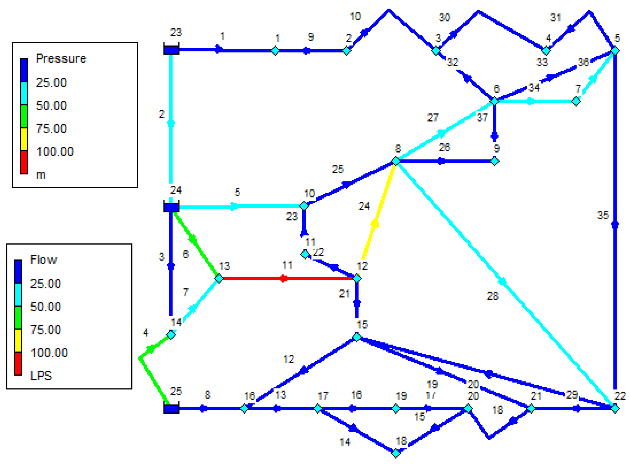
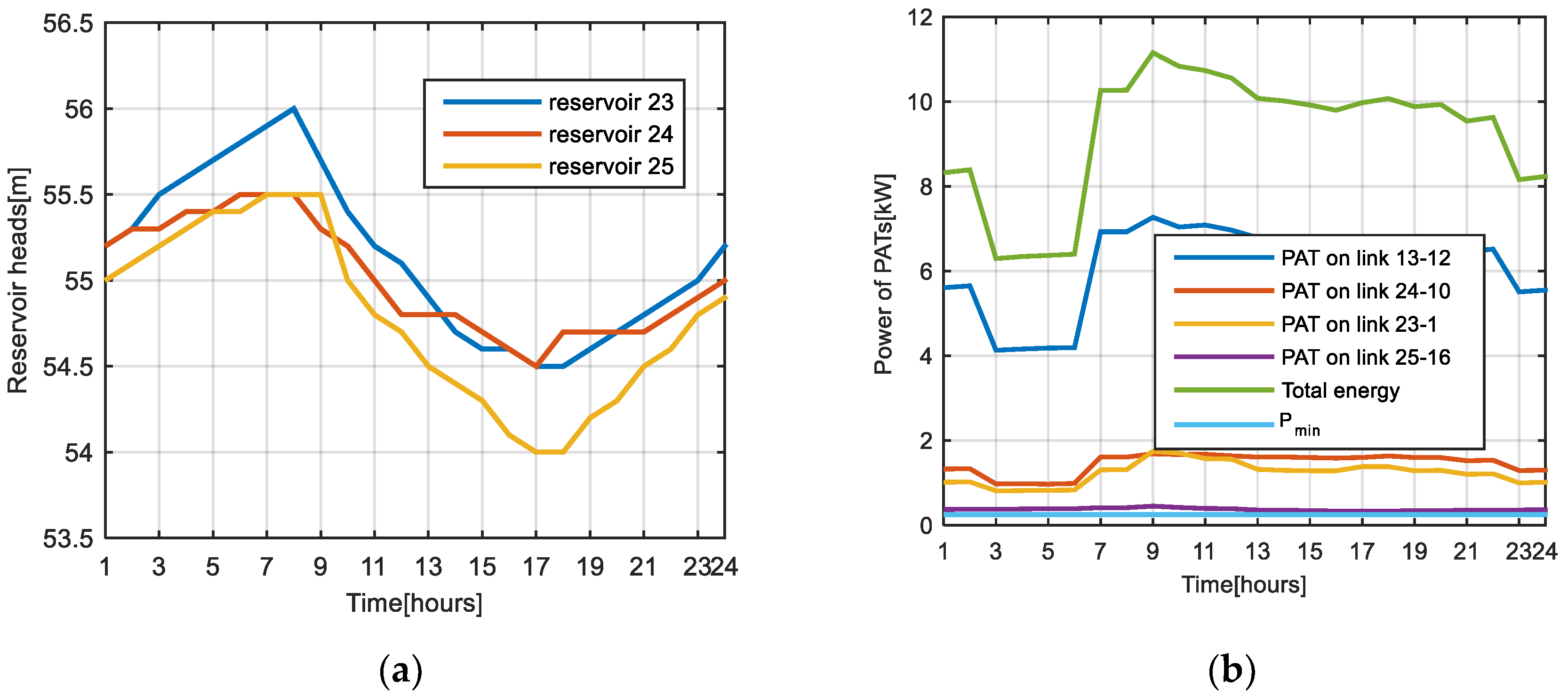
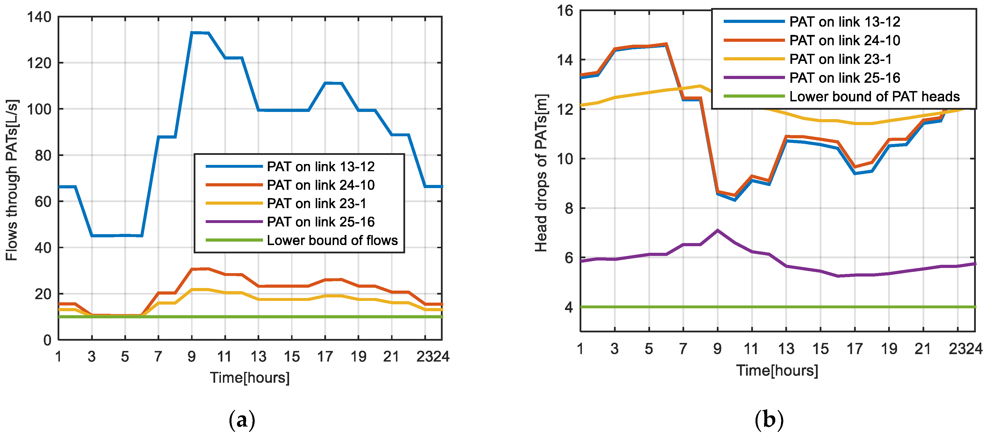
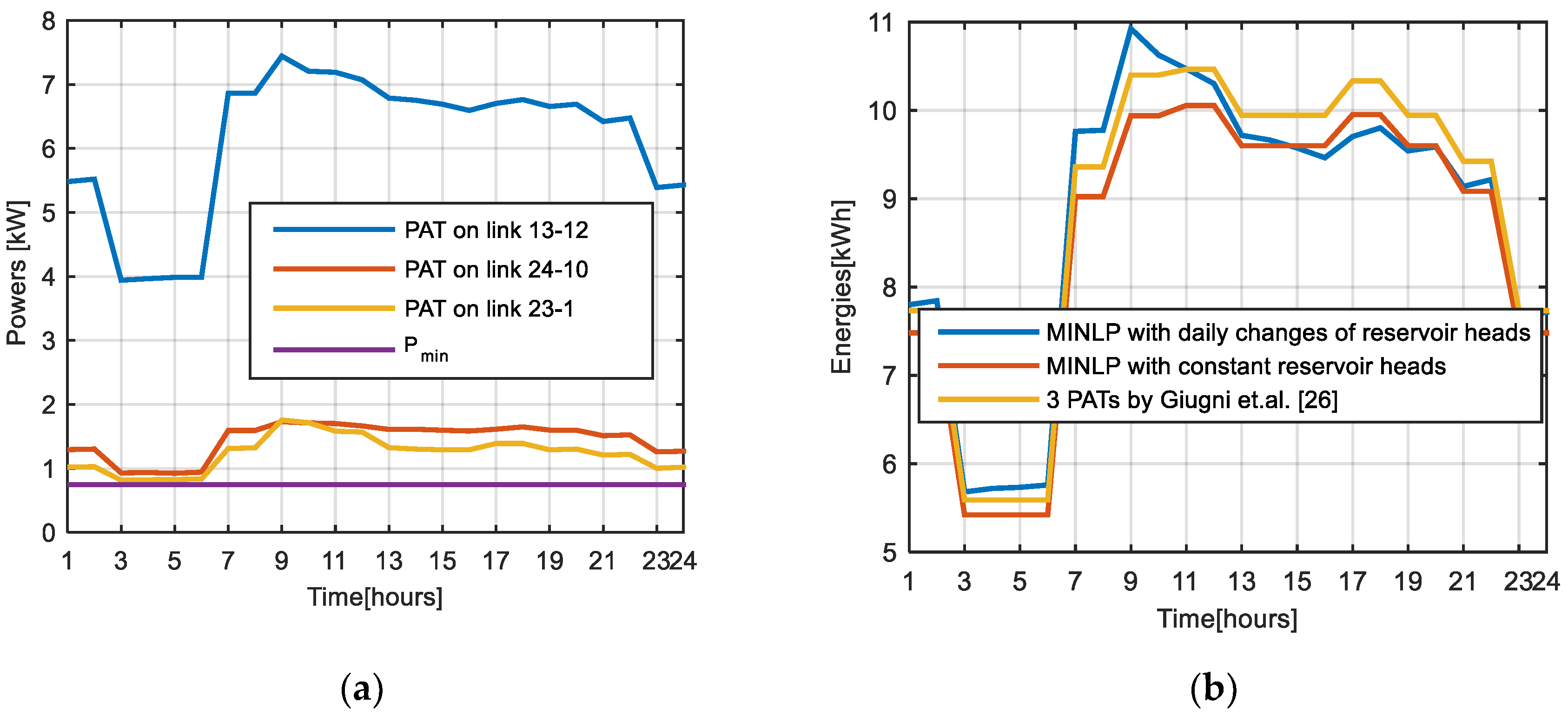
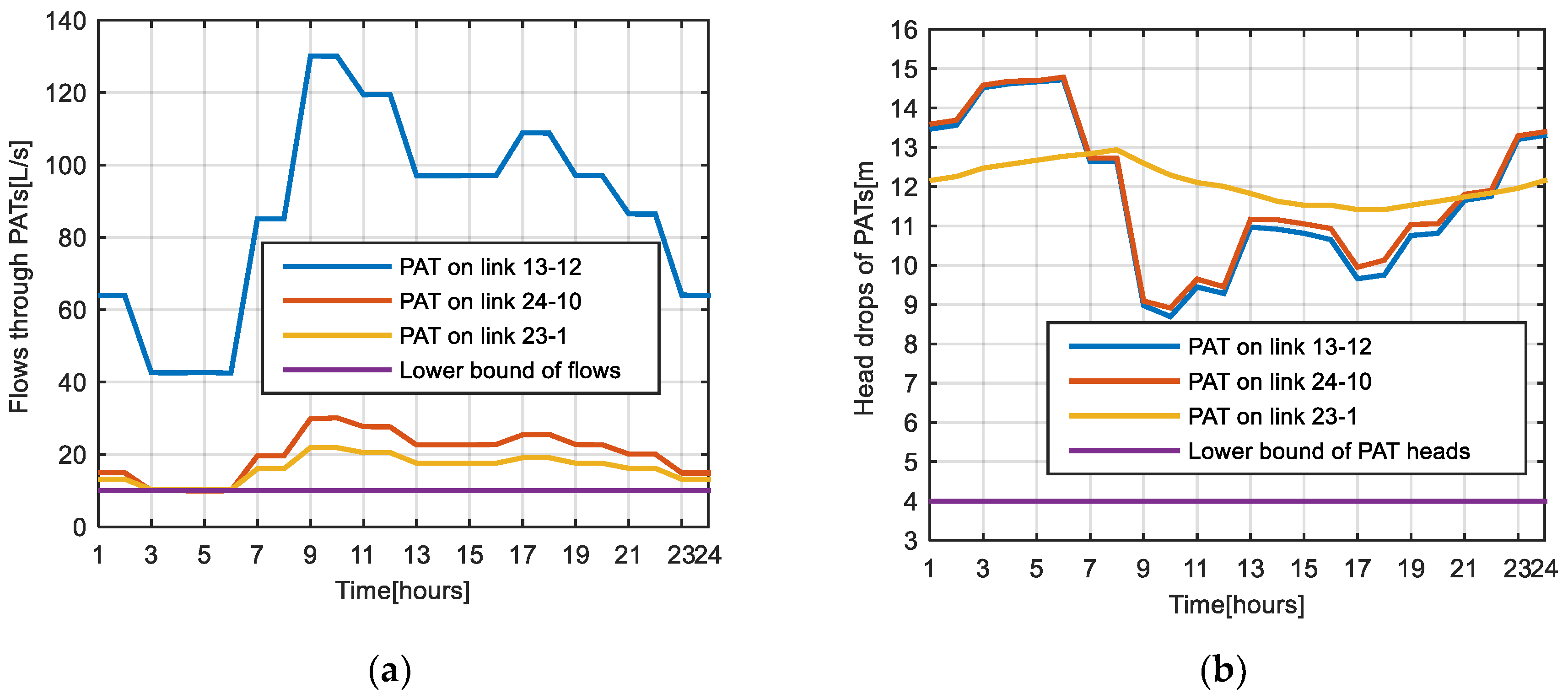
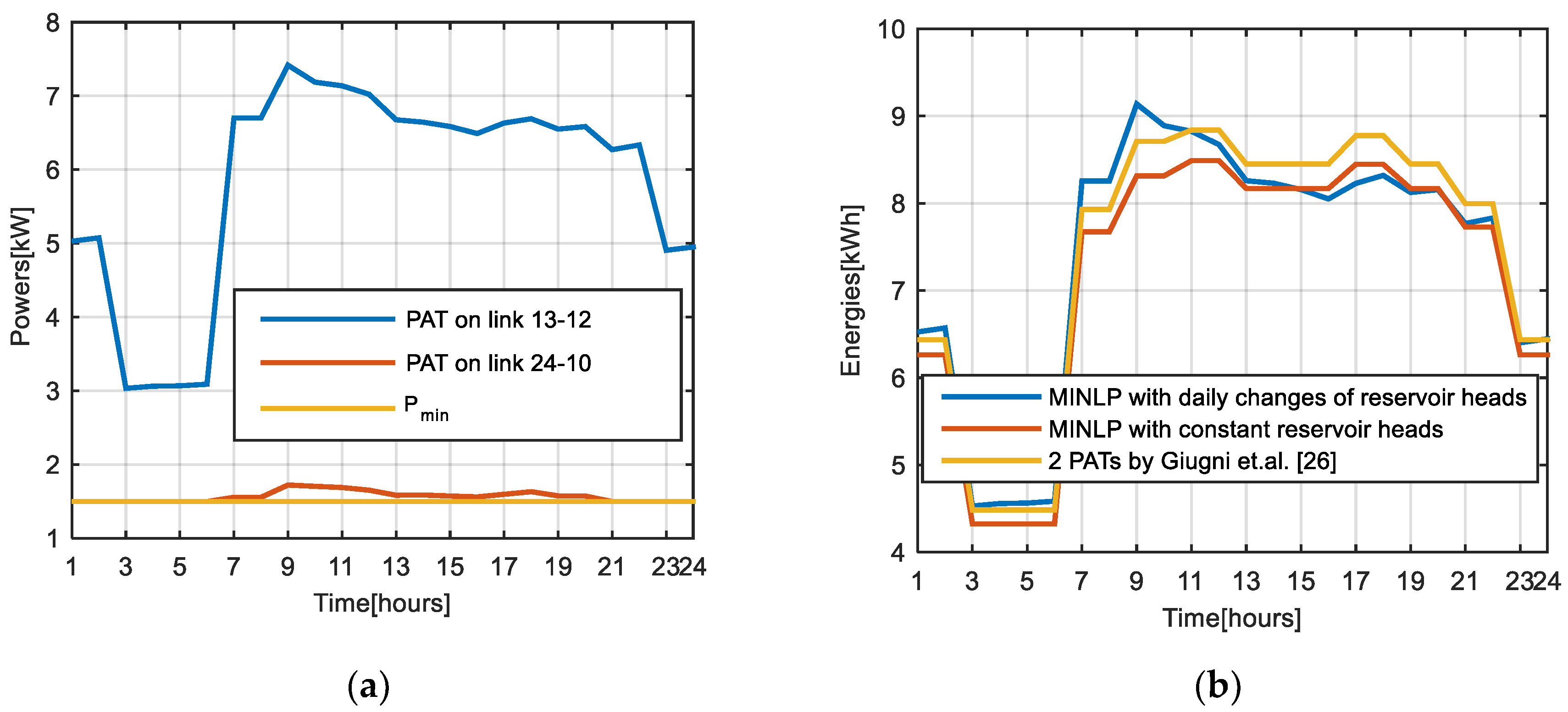
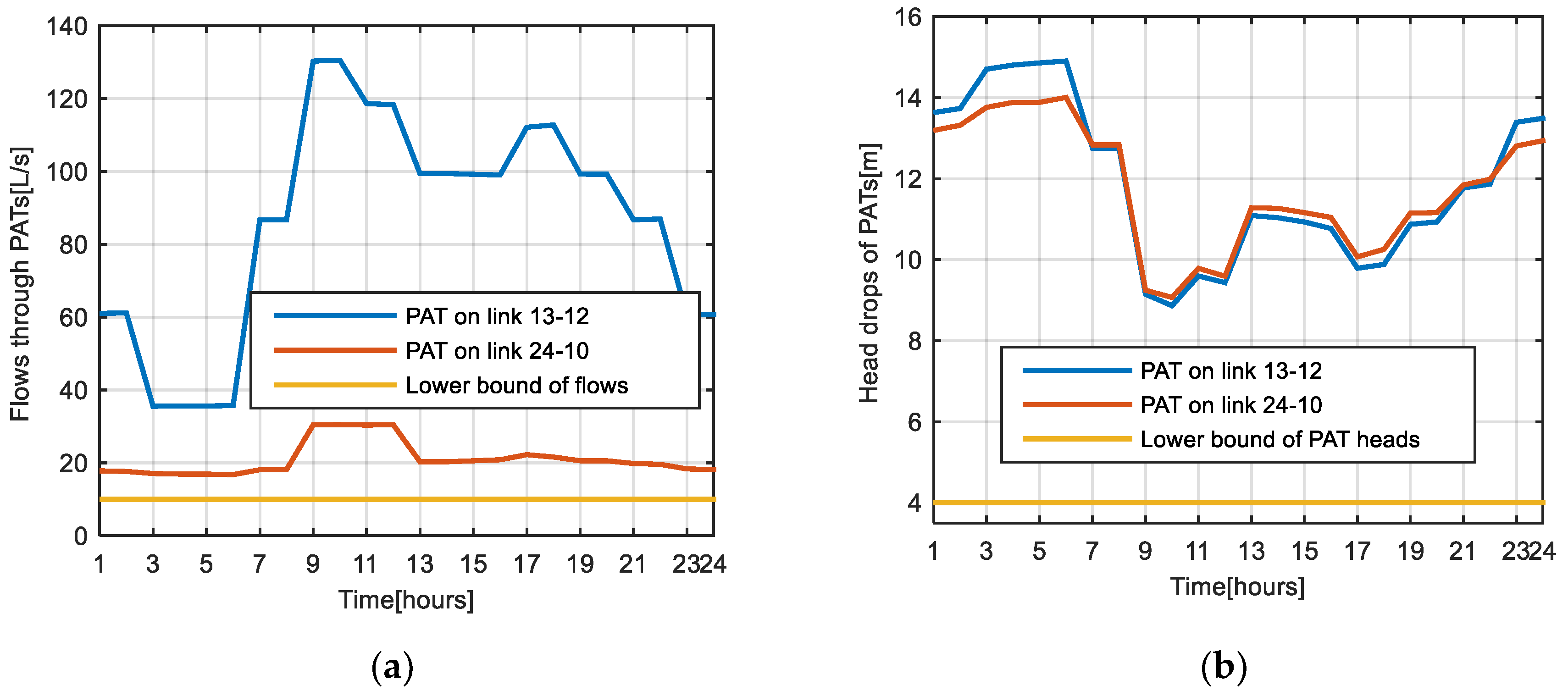
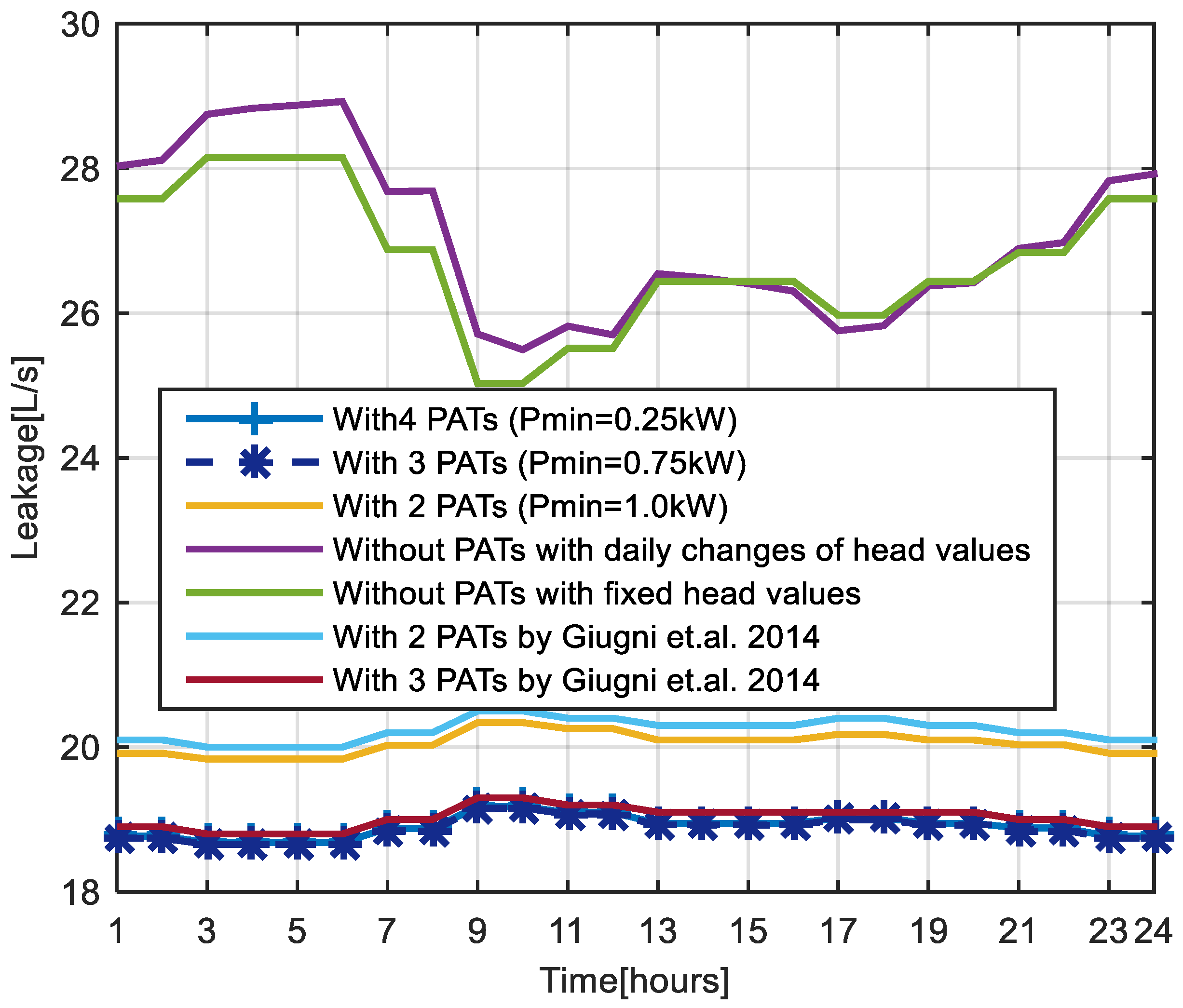
3.1. Case Study 1
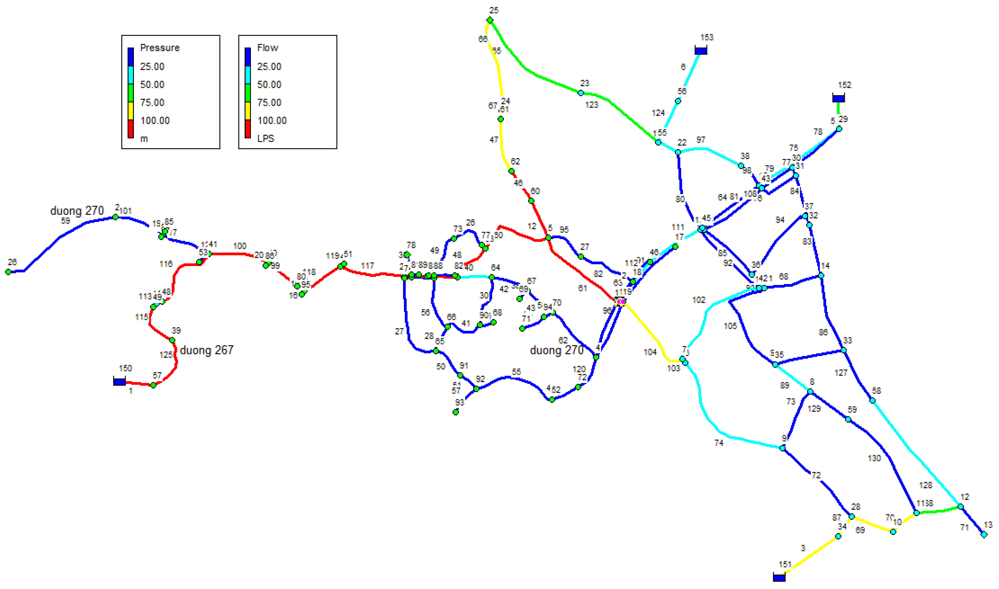
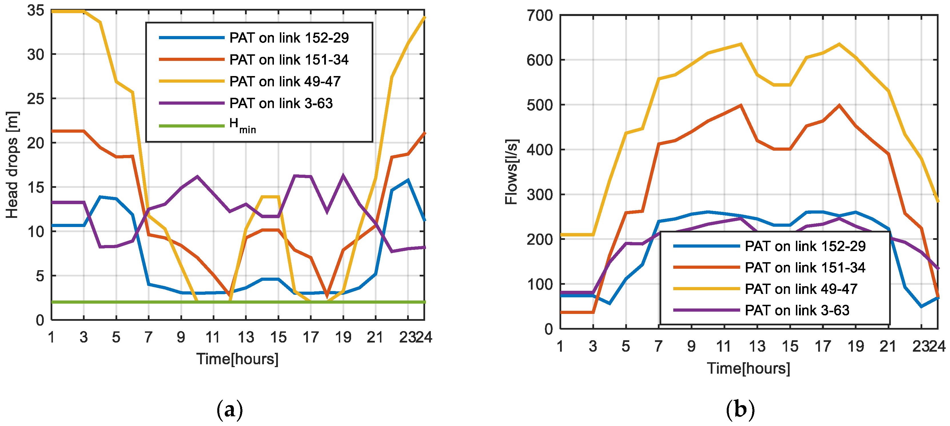
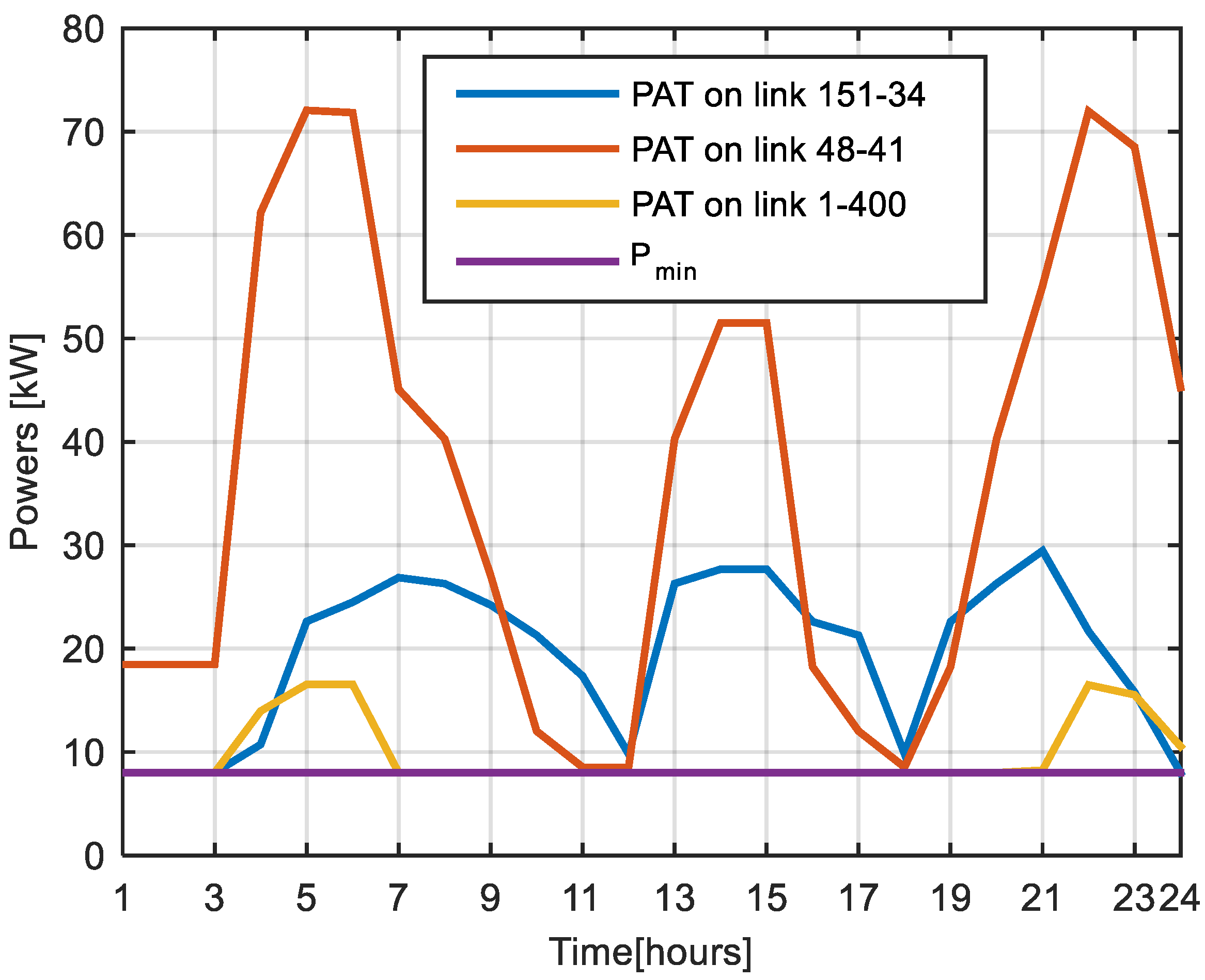
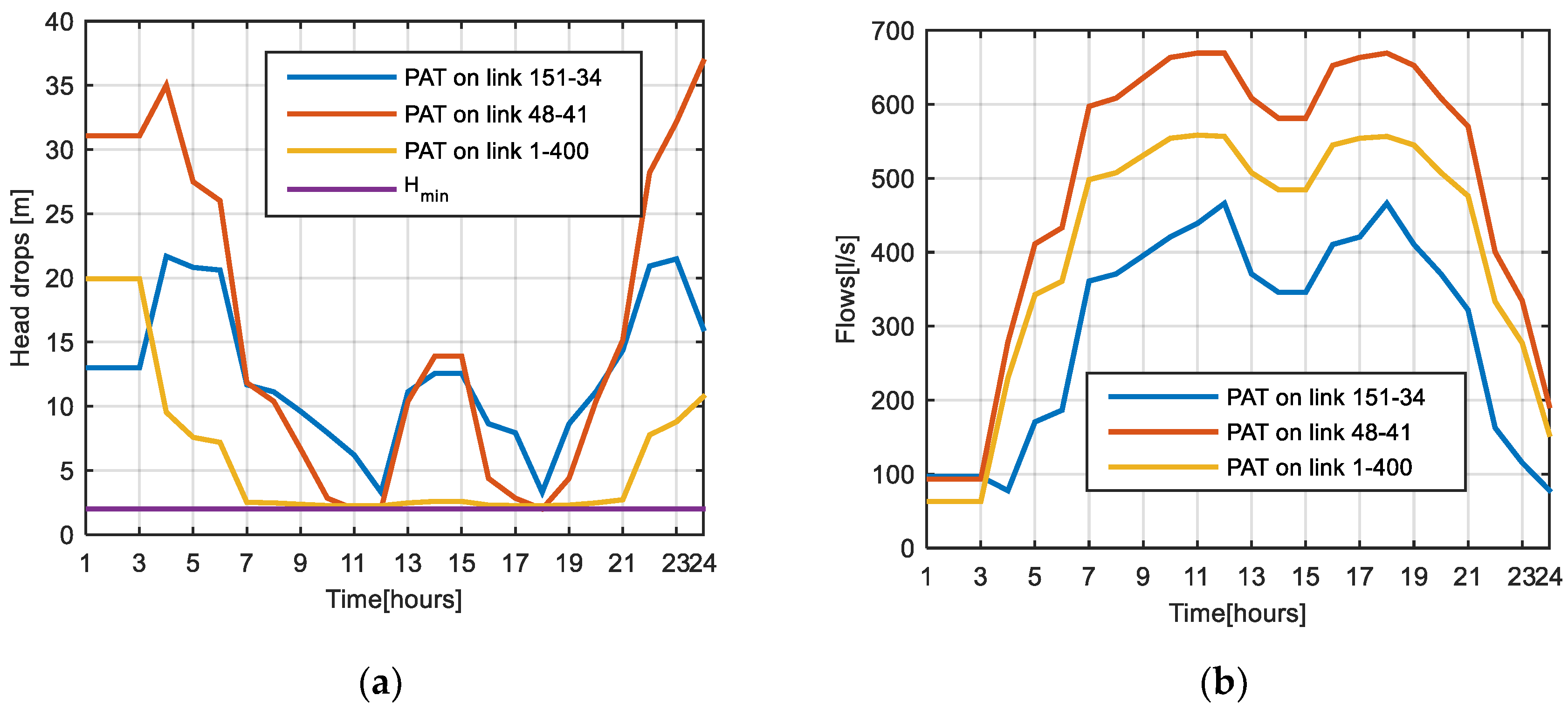
3.2. Case Study 2: Optimal Pressure Management for a Real-World WDS in a City in Vietnam
4. Conclusions
Author Contributions
Funding
Conflicts of Interest
Abbreviation
| Hazen-William Coefficient | |
| Discharge Coefficient of the Orifice | |
| Diameter and Hazen-William Coefficient (m) | |
| Demand at Node i at Time Interval k (m3/s) | |
| Average Excessive Pressure (m) | |
| Pipe Friction Factor | |
| Nodal Head at Node i at Time Interval k (m) | |
| Head Loss Across the Link ij at Time Interval k (m) | |
| Minimum Required value of the PATs Head Drop (m) | |
| Index of time Interval | |
| Leakage at node i at time Interval k (m3/s) | |
| Length of Link ij (m) | |
| Specified Minimum Power of PATs | |
| Average Power (m) | |
| Static Pressure at Node i at Time Interval k(m) | |
| Lower Bounds of Flows through PATs (m3/s) | |
| Upper Bounds of Flows through Links (m3/s) | |
| Flow Variables at time Interval k (m3/s) | |
| Tolerant Variable | |
| , | Binary Variables Representing Appearance of PATs on Link ij in Both Directions |
| Head Drop Across PATs at Time Interval k (m) | |
| Average Efficiency of the PAT | |
| Specific Weight of Water (N/m3) | |
| Leakage Exponent |
References
- Sterling, M.J.H.; Bargiela, A. Leakage reduction by optimised control of valves in water networks. Trans. Inst. Measur. Contr. 1984, 6, 293–298. [Google Scholar] [CrossRef]
- Araujo, L.S.; Ramos, H.; Coelho, S.T. Pressure control for leakage minimisation in water distribution systems management. Water Resour. Manag. 2006, 20, 133–149. [Google Scholar]
- Ulanicki, B.; Bounds, P.L.M.; Rance, J.P.; Reynolds, L. Open and closed loop pressure control for leakage reduction. Urban Water 2000, 2, 105–114. [Google Scholar] [CrossRef]
- Vairavamoorthy, K.; Lumbers, J. Leakage reduction in water distribution systems: Optimal valve control. J. Hydraul. Eng. 1998, 124, 1146–1154. [Google Scholar] [CrossRef]
- Eck, B.J.; Mevissen, M. Valve Placement in Water Networks: Mixed-Integer Non-Linear Optimization with Quadratic Pipe Friction; Report No. RC25307 (IRE1209-014); IBM Research: Armonk, NY, USA, 2012. [Google Scholar]
- Dai, P.D.; Li, P. Optimal localization of pressure reducing valves in water distribution systems by a reformulation approach. Water Res. Manag. 2014, 28, 3057–3074. [Google Scholar] [CrossRef]
- Nicolini, M.; Zovatto, L. Optimal location and control of pressure reducing valves in water networks. J. Water Res. Plan. Manag. 2009, 135, 178–187. [Google Scholar] [CrossRef]
- Liberatore, S.; Sechi, G.M. Location and calibration of valves in water distribution networks using a scatter-search meta-heuristic approach. Water Res. Manag. 2009, 23, 1479–1495. [Google Scholar] [CrossRef]
- Pecci, F.; Abraham, E.; Stoianov, I. Outer approximation methods for the solution of co-design optimisation problems in water distribution networks. IFAC Pap. Online 2017, 50, 5373–5379. [Google Scholar] [CrossRef]
- Pecci, F.; Abraham, E.; Stoianov, I. Model reduction and outer approximation for optimizing the placement of control valves in complex water networks. J. Water Resour. Plan. Manag. 2019, 145, 04019014. [Google Scholar] [CrossRef]
- Pecci, F.; Abraham, E.; Stoianov, I. Global optimality bounds for the placement of control valves in water supply networks. Optim. Eng. 2019, 20, 457–495. [Google Scholar] [CrossRef]
- Cao, H.; Hopfgarten, S.; Ostfeld, A.; Salomons, E.; Li, P. Simultaneous Sensor Placement and Pressure Reducing Valve Localization for Pressure Control of Water Distribution Systems. Water 2019, 11, 1352. [Google Scholar] [CrossRef]
- Fontana, N.; Giugni, M.; Portolano, D. Losses reduction and energy production in water-distribution networks. J. Water Resour. Plan. Manag. 2012, 138, 237–244. [Google Scholar] [CrossRef]
- Kramer, M.; Terheiden, K.; Wieprecht, S. Pumps as turbines for efficient energy recovery in water supply networks. Renew. Energy 2018, 122, 17–25. [Google Scholar] [CrossRef]
- Pugliese, F.; De Paola, F.; Fontana, N.; Giugni, M.; Marini, G. Experimental characterization of two Pumps As Turbines for hydropower generation. Renew. Energy 2016, 99, 180–187. [Google Scholar] [CrossRef]
- Corcoran, L.; McNabola, A.; Coughlan, P. Optimization of water distribution networks for combined hydropower energy recovery and leakage reduction. J. Water Resour. Plan. Manag. 2016, 142, 04015045. [Google Scholar] [CrossRef]
- Fecarotta, O.; McNabola, A. Optimal location of pump as turbines (PATs) in water distribution networks to recover energy and reduce leakage. Water Resour. Manag. 2017, 31, 5043–5059. [Google Scholar] [CrossRef]
- Carravetta, A.; Del Giudice, G.; Fecarotta, O.; Ramos, H.M. Energy production in water distribution networks: A PAT design strategy. Water Resour. Manag. 2012, 26, 3947–3959. [Google Scholar] [CrossRef]
- Carravetta, A.; Del Giudice, G.; Fecarotta, O.; Ramos, H.M. PAT design strategy for energy recovery in water distribution networks by electrical regulation. Energies 2013, 6, 411–424. [Google Scholar] [CrossRef]
- Puleo, V.; Fontanazza, C.M.; Notaro, V.; De Marchis, M.; Freni, G.; La Loggia, G. Pumps as turbines (PATs) in water distribution networks affected by intermittent service. J. Hydroinform. 2014, 16, 259–271. [Google Scholar] [CrossRef]
- Carravetta, A.; Fecarotta, O.; Sinagra, M.; Tucciarelli, T. Cost-benefit analysis for hydropower production in water distribution networks by a pump as turbine. J. Water Resour. Plan. Manag. 2014, 140, 04014002. [Google Scholar] [CrossRef]
- Fecarotta, O.; Aricò, C.; Carravetta, A.; Martino, R.; Ramos, H.M. Hydropower potential in water distribution networks: Pressure control by PATs. Water Resour. Manag. 2015, 29, 699–714. [Google Scholar] [CrossRef]
- De Marchis, M.; Milici, B.; Volpe, R.; Messineo, A. Energy saving in water distribution network through pump as turbine generators: Economic and environmental analysis. Energies 2016, 9, 877. [Google Scholar] [CrossRef]
- Samora, I.; Manso, P.; Franca, M.; Schleiss, A.; Ramos, H. Energy Recovery Using Micro-Hydropower Technology in Water Supply Systems: The Case Study of the City of Fribourg. Water 2016, 8, 344. [Google Scholar] [CrossRef]
- Parra, S.; Krause, S.; Krönlein, F.; Günthert, F.W.; Klunke, T. Intelligent pressure management by pumps as turbines in water distribution systems: Results of experimentation. Water Sci. Technol. Water Supply 2018, 18, 778–789. [Google Scholar] [CrossRef]
- Giugni, M.; Fontana, N.; Ranucci, A. Optimal location of PRVs and turbines in water distribution systems. J. Water Resour. Plan. Manag. 2014, 140, 06014004. [Google Scholar] [CrossRef]
- Jafari, R.; Khanjani, M.J.; Esmaeilian, H.R. Pressure management and electric power production using pumps as turbines. J. Am. Water Works Assoc. 2015, 107, E351–E363. [Google Scholar] [CrossRef]
- Rossman Lewis, A. EPANET 2: User’s Manual; US Environmental Protection Agency: Washington, DC, USA; Office of Research and Development: Washington, DC, USA; National Risk Management Research Laboratory: Washington, DC, USA, 2000.
- Lima, G.M.; Junior, E.L.; Brentan, B.M. Selection and location of Pumps as Turbines substituting pressure reducing valves. Renew. Energy 2017, 109, 392–405. [Google Scholar] [CrossRef]
- Lima, G.M.; Luvizotto, E., Jr.; Brentan, B.M.; Ramos, H.M. Leakage control and energy recovery using variable speed pumps as turbines. J. Water Resour. Plan. Manag. 2018, 144, 04017077. [Google Scholar] [CrossRef]
- Tricarico, C.; Morley, M.S.; Gargano, R.; Kapelan, Z.; Savić, D.; Santopietro, S.; Granata, F.; de Marinis, G. Optimal energy recovery by means of pumps as turbines (PATs) for improved WDS management. Water Sci. Technol. Water Supply 2018, 18, 1365–1374. [Google Scholar] [CrossRef]
- Carravetta, A.; Derakhshan Houreh, S.; Ramos, H.M. Pumps as Turbines: Fundamentals and Applications; Springer: Berlin, Germany, 2018. [Google Scholar]
- Jain, S.V.; Patel, R.N. Investigations on pump running in turbine mode: A review of the state-of-the-art. Renew. Sustain. Energy Rev. 2014, 30, 841–868. [Google Scholar] [CrossRef]
- Belotti, P.; Kirches, C.; Leyffer, S.; Linderoth, J.; Luedtke, J.; Mahajan, A. Mixed-integer nonlinear optimization. Acta Numer. 2013, 22, 1–131. [Google Scholar] [CrossRef]
- Bonami, P.; Biegler, L.T.; Conn, A.R.; Cornuéjols, G.; Grossmann, I.E.; Laird, C.D.; Lee, J.; Lodi, A.; Margot, F.; Sawaya, N.; et al. An algorithmic framework for convex mixed integer nonlinear programs. Discret. Optim. 2008, 5, 186–204. [Google Scholar] [CrossRef]
- Brook, A.; Kendrick, D.; Meeraus, A. GAMS, a user’s guide. ACM Signum Newsl. 1988, 23, 10–11. [Google Scholar] [CrossRef]
- Rossman, L. AEPANET 2 Users Manual, Rep. EPA/600/R-00/057; U.S. Environ. Prot. Agency: Cincinnati, OH, USA, 2000.


| Time (h) | Demand Pattern Factors | Time (h) | Demand Pattern Factors |
|---|---|---|---|
| 1 | 0.61 | 13 | 0.92 |
| 2 | 0.61 | 14 | 0.92 |
| 3 | 0.41 | 15 | 0.92 |
| 4 | 0.41 | 16 | 0.92 |
| 5 | 0.41 | 17 | 1.03 |
| 6 | 0.41 | 18 | 1.03 |
| 7 | 0.81 | 19 | 0.92 |
| 8 | 0.81 | 20 | 0.920 |
| 9 | 1.23 | 21 | 0.82 |
| 10 | 1.23 | 22 | 0.82 |
| 11 | 1.13 | 23 | 0.61 |
| 12 | 1.13 | 24 | 0.61 |
| Scenarios Pmin | PAT Locations | Computation Time (s) |
|---|---|---|
| 0.25 kW | 25–16; 24–10; 23–1; 13–12 | 3542.20 |
| 0.75 kW | 24–10; 23–1; 13–12 | 1537.86 |
| 1.0 kW | 24–10; 13–12 | 2185.59 |
| 1.2 kW | 24–10; 13–12 | 26.38 |
| 1.5 kW | 24–10; 13–12 | 1224.92 |
| Our MINLP Model | Giugni et al. [26] | |||||
|---|---|---|---|---|---|---|
| Daily Changes of Water Levels in Reservoirs | Constant Water Levels in Reservoirs | Constant Water Levels in Reservoirs | ||||
| Scenarios Pmin | Electrical Energy (kWh/day) | Average Leakage Reduction (L/s) | Electrical Energy (kWh/day) | Average Leakage Reduction (L/s) | Electrical Energy (kWh/day) | Average Leakage Reduction (L/s) |
| 1.5 kW (2PATs) | 177.33 | 6.93 | 172.65 | 6.70 | 178.88 | 6.50 |
| 0.75 kW (3PATs) | 211.18 | 8.02 | 205.31 | 7.88 | 212.94 | 7.72 |
| 0.25 kW (4PATs) | 221.20 | 8.14 | 218.40 | 7.85 | - | - |
| Time (h) | Demand Pattern Factors | Time (h) | Demand Pattern Factors |
|---|---|---|---|
| 1 | 0.36 | 13 | 1.2 |
| 2 | 0.36 | 14 | 1.15 |
| 3 | 0.36 | 15 | 1.15 |
| 4 | 0.58 | 16 | 1.28 |
| 5 | 0.82 | 17 | 1.30 |
| 6 | 0.86 | 18 | 1.34 |
| 7 | 1.18 | 19 | 1.28 |
| 8 | 1.20 | 20 | 1.20 |
| 9 | 1.25 | 21 | 1.12 |
| 10 | 1.30 | 22 | 0.80 |
| 11 | 1.32 | 23 | 0.68 |
| 12 | 1.34 | 24 | 0.46 |
| Scenarios Pmin | PAT Locations | Computation Time (s) | Pav (kW) | Produced Energy (kWh/day) | EX (m) |
|---|---|---|---|---|---|
| No PATs | - | - | - | 23.73 | |
| 5.0 kW | 3–63; 49–47; 151–34; 152–29 | 57,684.10 | 83.14 | 1995.46 | 12.77 |
| 8.0 kW | 48–41; 151–34; 1–400 | 43,202.60 | 66.62 | 1599.00 | 12.79 |
| 12.0 kW | 41–40 | 11,394.0 | 48.52 | 1164.62 | 17.35 |
© 2020 by the authors. Licensee MDPI, Basel, Switzerland. This article is an open access article distributed under the terms and conditions of the Creative Commons Attribution (CC BY) license (http://creativecommons.org/licenses/by/4.0/).
Share and Cite
Nguyen, K.D.; Duc Dai, P.; Quoc Vu, D.; Cuong, B.M.; Tuyen, V.P.; Li, P. A MINLP Model for Optimal Localization of Pumps as Turbines in Water Distribution Systems Considering Power Generation Constraints. Water 2020, 12, 1979. https://doi.org/10.3390/w12071979
Nguyen KD, Duc Dai P, Quoc Vu D, Cuong BM, Tuyen VP, Li P. A MINLP Model for Optimal Localization of Pumps as Turbines in Water Distribution Systems Considering Power Generation Constraints. Water. 2020; 12(7):1979. https://doi.org/10.3390/w12071979
Chicago/Turabian StyleNguyen, Khoa Dang, Pham Duc Dai, Dong Quoc Vu, Bui Manh Cuong, Vu Phi Tuyen, and Pu Li. 2020. "A MINLP Model for Optimal Localization of Pumps as Turbines in Water Distribution Systems Considering Power Generation Constraints" Water 12, no. 7: 1979. https://doi.org/10.3390/w12071979
APA StyleNguyen, K. D., Duc Dai, P., Quoc Vu, D., Cuong, B. M., Tuyen, V. P., & Li, P. (2020). A MINLP Model for Optimal Localization of Pumps as Turbines in Water Distribution Systems Considering Power Generation Constraints. Water, 12(7), 1979. https://doi.org/10.3390/w12071979