Drought Index as Indicator of Salinization of the Salento Aquifer (Southern Italy)

Abstract

Salento peninsula (Southern Italy) hosts a coastal carbonate and karst aquifer. The semi-arid climate is favourable to human settlement and the development of tourism and agricultural activities, which involve high water demand and groundwater exploitation rates, in turn causing groundwater depletion and salinization. In the last decades these issues worsened because of the increased frequency of droughts, which emerges from the analysis of Standardized Precipitation Index (SPI), calculated during 1949–2011 on the base of monthly precipitation. Groundwater level series and chloride concentrations, collected over the extreme drought period 1989–1990, allow a qualitative assessment of groundwater behaviour, highlighting the concurrent groundwater drought and salinization.

1. Introduction

In 2017 the European Environment Agency (EEA) [1] indicated that droughts are projected to increase in frequency, duration and severity in most of Europe, while the greatest increase is expected for Southern Europe. Under the A2 emissions scenario of IPCC [2] it is expected that all of Italy will go through significant drying and that precipitation will decrease by about 10% to over 40% in the summer [3]. Records show that the average temperature of Europe [4] has risen by 0.95 °C over the last century (1901–2001) and that climate change has caused a steepening of precipitation and temperature gradients resulting in wetter conditions in northern regions and drier conditions in southern areas. Thus, the climate change (i.e., changes in precipitation, total runoff, temperature, potential evapotranspiration) and recurrent drought periods will significantly affect freshwater resources stored in rivers, lakes and aquifers.

The decrease in potential groundwater recharge in Southern Europe [5] should have a severe impact on the availability of freshwater resources for drinking and irrigation uses. Thus, concerning water resources, climate change may have a series of cascading consequences and originate feedback loops, as well as changes in land use [6] that lead to a variation of evapotranspiration. It should be expected that the projected reduction of soil moisture storage will first produce a decrease of groundwater recharge and, later, a decline of groundwater levels and discharge.

In this framework droughts play a key role in understanding environmental complex dynamics [7]. Consistently to the different phenomenologies, they can be classified into four categories [8,9,10]: (i) meteorological, which refers to a lack of precipitation in a large area and over a long period of time; (ii) agricultural (also called soil moisture), which depends on a deficiency of soil moisture, usually in the root zone; (iii) hydrological, associated to negative anomalies in surface and sub-surface water; and (iv) socio-economic, due to a failure of water resources systems concerning water demands and ecological or health-related impacts. When a combination of the above-mentioned types of droughts occurs at the same time in a certain area it can generate a so-called groundwater drought [11].

Generally, by using frequency analysis of historical data, a groundwater drought is defined as the lack of groundwater, expressed in terms of recharge, storage or hydraulic heads in a certain area and over a particular period of time [12] compared to “normal” conditions (average amount or level). However, an increase of groundwater abstraction occurs during prolonged dry periods or droughts: in the Mediterranean regions, the quite diffuse imbalance between water-demand and water availability (especially due to agricultural sector) may then enhance naturally occurring droughts. Over-exploitation reduces groundwater quantity, leaving aquifers without an efficient storage to cover dry periods [13].

Notwithstanding the potential and serious drawbacks of “superficial” droughts and the knowledge that the effects of primary meteorological drought events are destined to propagate on the entire water cycle [12], groundwater is considered a resilient resource during periods of lower than average rainfall. During the initial phases of a drought, indeed, groundwater can provide relatively resilient water supplies and will sustain surface flows through groundwater baseflow [14]. On the other hand, groundwater may be highly vulnerable to protracted droughts, since groundwater storage may need a longer time to be restocked and recover in comparison to surface water resources as a drought starts to break.

If we consider the complex character of the dependence between groundwater and groundwater-dependent (natural and urban) ecosystems, a worsening in quality and quantity of the former can generate cascading consequences and crises on the latter. In light of water management, such complex and strong interconnections and the possible high delays in the onset of a groundwater drought compared to the superficial drought, when unidentified, raise serious issues about the potential secondary emergencies and cascading vulnerabilities on groundwater-dependent systems.

In the Mediterranean area most of the population resides in the coastal zone, relying on groundwater in coastal aquifers. They are characterized by fresh groundwater floating on salt water due to a different fluid density and may also contain great amounts of water of very good quality, which are, today, subject to alarming salinization processes [15] due to exploitation and/or reduced recharge. Under a decrease of water levels, the transition zone expands, thus reducing the thickness of fresh water with a concurrent increase in its salt content. Depending on the aquifer scale, groundwater takes different times to recover to the previous water level. However, even if after a drought period a normal wet period leads to recovered levels, groundwater quality often remains compromised because exploitation normally does not stop.

An exponential rise of groundwater drawings favours and accelerates this phenomenon due to the attempt to bridge the gap between the increasing water demand and the water availability.

Groundwater in the coastal aquifer of Salento (Puglia, Southern Italy) is highly vulnerable to salinization because of the structure of the aquifer, where discontinuities and karst forms are ways of fast and deep intrusion for seawater and saltwater [16]. In Salento, droughts may easily propagate their effects to the coastal aquifer, worsening qualitative and quantitative status of groundwater and causing cascade crisis [17]. This situation is currently threatened by climate change, which is leading to an increase in groundwater exploitation as in other areas typified by a high level of urbanization and low natural availability of water resources [18]. In the Adriatic and Ionian coastal zones of Salento there is, in fact, an increasing aridity, which impacts on water demand for irrigated agriculture [19].

This study aims as first at representing the drought scenario of the karst coastal aquifer of Salento (Puglia region, Southern Italy) between 1949 and 2011. Then, in correspondence with a period characterized by extreme droughts, the study will show and discuss data about the response of groundwater at four monitoring wells, concerning both its quantitative and qualitative status, with the aim of understanding what the relationships between meteorological and groundwater droughts are. Section 2 describes the meaning and main characteristics of the current drought indicators, while Section 3 illustrates the case study of Salento, with details about dataset problems. Section 4 deals with the methodology adopted for computing SPI and resulting trends; Section 5 shows results and Section 6 discusses related hydrogeological implications, highlighting the main findings. Finally, paragraph 7 outlines the main conclusions of this study.

2. Drought Indicators

Literature proposes numerous methods for calculating meteorological drought indices aimed at quantifying and comparing drought severity, as well as its duration and extent across a certain area and during years. Nowadays, there is not a common method that is suitable for all circumstances and users [20].

The Standardised Precipitation Index (SPI) is among the most used meteorological indices [21]: the World Meteorological Organization considers SPI the best suitable indicator of wetness or dryness conditions [22]. The calculation of SPI requires monthly precipitation, ideally for a continuous period of at least 30 years; it consists of a normalized index with zero mean and standard deviation of one, obtained by fitting a gamma distribution to long-term records of monthly precipitation to represent the relationship of probability to precipitation. Usually, accumulation periods of precipitation are used to estimate the index for different timescales, typically 1, 3, 6, 12 and 24 months; at longer timescales, drought frequencies decrease and consequently drought durations increase. Thus, accumulation precipitations of: (i) 1–3–6 months are used to account agricultural drought; (ii) 12 months to evaluate hydrological drought; and (iii) 24-months to define socio-economic impacts [23]. Successively, to obtain SPI, the corresponding cumulative probability distribution is computed and transformed to the standard normal distribution. Positive values of SPI indicate wet conditions, while negative values refer to dry conditions; an extreme drought occurs when SPI is less than −2. The SPI approach includes several strengths: the use of a unique input data (precipitation), although it requires a long and continuous precipitation time series, the possibility to estimate the index for a variety of timescales, and the feasibility of comparison with other indicators.

The more recently proposed Standardised Precipitation-Evapotranspiration Index (SPEI) [24,25] is similar to SPI in the mathematical structure. Differently from SPI, that uses the precipitation as input, SPEI is calculated from normalized accumulated climatic water balance anomalies, defined as the difference between precipitation and potential evapotranspiration (PET). Then, accumulated water balance is transformed to probabilities and finally converted to the standard normal distribution for computing drought index values. It is important to remark that potential evapotranspiration is the amount of evaporation and transpiration that would occur if a sufficient water source is available. It can be calculated with three approaches: (i) the Thornthwaite method [26], which is the simplest method because it needs only of monthly mean temperature registrations and latitude of the site; (ii) the Hargreaves method [27], that computes the monthly reference evapotranspiration (ET0) of a grass crop and requires minimum and maximum temperature registrations and latitude of the site; and (iii) Penman–Monteith method, that according to Allen et al. [28] calculates ET0 of a hypothetical reference crop, known minimum and maximum temperature registrations and time series of monthly mean daily external radiation, monthly mean daily wind speeds at 2 m height, monthly mean daily bright sunshine hours and monthly mean cloud cover in percentage. The original formulation of SPEI [24] suggests using Thornthwaite method to calculate potential evapotranspiration because of its simplicity, but previous studies demonstrate that this approach underestimates PET in arid and semiarid region. Thus, the Food and Agriculture Organization of the United Nations (FAO) and the American Society of Civil Engineers (ASCE) advised the use of the Penman–Monteith formulation [29,30]. Furthermore, with regard to the Hargreaves formulation, as for the Thornthwaite method, it needs limited data, and it is demonstrated that at monthly and annual timescales PET estimates do not differ significantly from the Penman–Monteith equations, with differences less than 2 mm per day [30]. SPI and SPEI indices are statistically interpretable, representing the number of standard deviations from typical accumulated precipitation, or climatic water balance, for a given location and time of year [31].

The Rainfall Anomaly Index (RAI) was developed by Van Rooy [32]. The RAI calculation can be developed for weekly, monthly or annual timescales, according to dry period frequency: in areas with short dry periods, a smaller timescale is used than in areas with long, dry periods. RAI is calculated arranging precipitations in descending order and selecting the ten highest values and the ten lowest ones from which the average values are computed to represent the thresholds for respectively positive and negative anomalies.

The Palmer Drought Severity Index (PDSI), developed by Palmer [33] for providing an index based on drought severity, allows the comparison of droughts with different time and spatial scales. It belongs to agricultural drought indicators, although many authors classify it as a meteorological one [34,35]. This index evaluates droughts according to the quantity of water stored in the unsaturated zone; therefore, it takes into account precipitation, evapotranspiration and soil moisture. Palmer method starts with a monthly or weekly water balance, using precipitation and temperature time series and contains many assumptions, which make it quite involved [35]. To account for soil moisture, the soil model considers two layers and two simplifications: the former is that the top layer can store 25 mm of water and the underlying layer has an available capacity according to local soil characteristics, whereas the latter is that all water in the first layer is used before the second layer starts leaving water.

All these indicators are climate-linked: they only highlight the influence of precipitation and air temperature on groundwater, but do not represent what may occur to this system. For the calculation of groundwater droughts, the Groundwater Resource Index (GRI) [36] was tested in Calabria, Southern Italy. It represents the normal distribution of the simulated groundwater storage of the Calabria region for 40-years of simulated data. Simulated data were generated by a hydrological model, based on precipitation, air temperature and air pressure as data input. Mendicino et al. [36], by comparing GRI with the SPI of 6, 12 and 24 months, find that the GRI was a better indicator than SPI for droughts in the Mediterranean area. They concluded that this approach appears a stable operative support for decision making when severe droughts and water scarcity problems occur because it is able to account for different information regarding meteorological, hydrological and agricultural aspects.

Regarding groundwater droughts, groundwater level time series can be converted into the Standardised Ground-water level Index (SGI) [37] using a non-parametric normal score transformation of groundwater level data for each calendar month. These monthly estimations are then merged to form a continuous index that is built on the SPI approach. This methodology shows how qualitative information on groundwater use and annual long-term averages help getting a better understanding of an asymmetric impact of groundwater use on groundwater droughts [38].

The requested variables for computing the above-described indices are summarized in

Table 1. Indices and linked variables.

Index	Hydrological Variable	Timescale
Standard Precipitation Index (SPI)	Rainfall	Monthly
Standardised Precipitation-Evapotranspiration Index (SPEI)	Rainfall, Temperature	Monthly
Rainfall Anomaly Index (RAI)	Rainfall	Weekly, monthly or annual
Palmer Drought Severity Index (sc-PDSI)	Rainfall, PET	Monthly
Palmer Drought Severity Index (PDSI)	Rainfall, Evaporation	Monthly

.

3. Study Area and Dataset

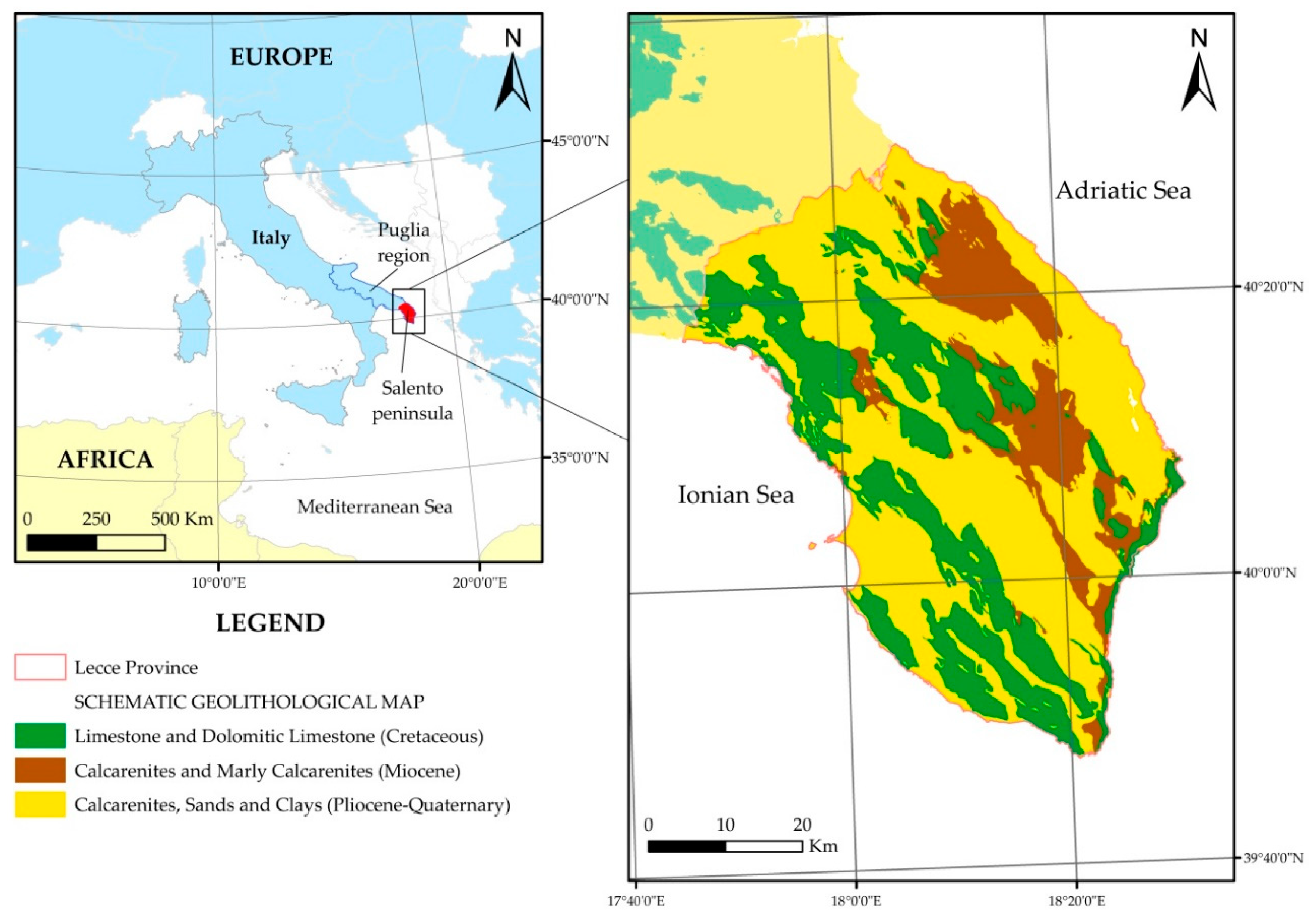
3.1. Geological and Hydrogeological Framework

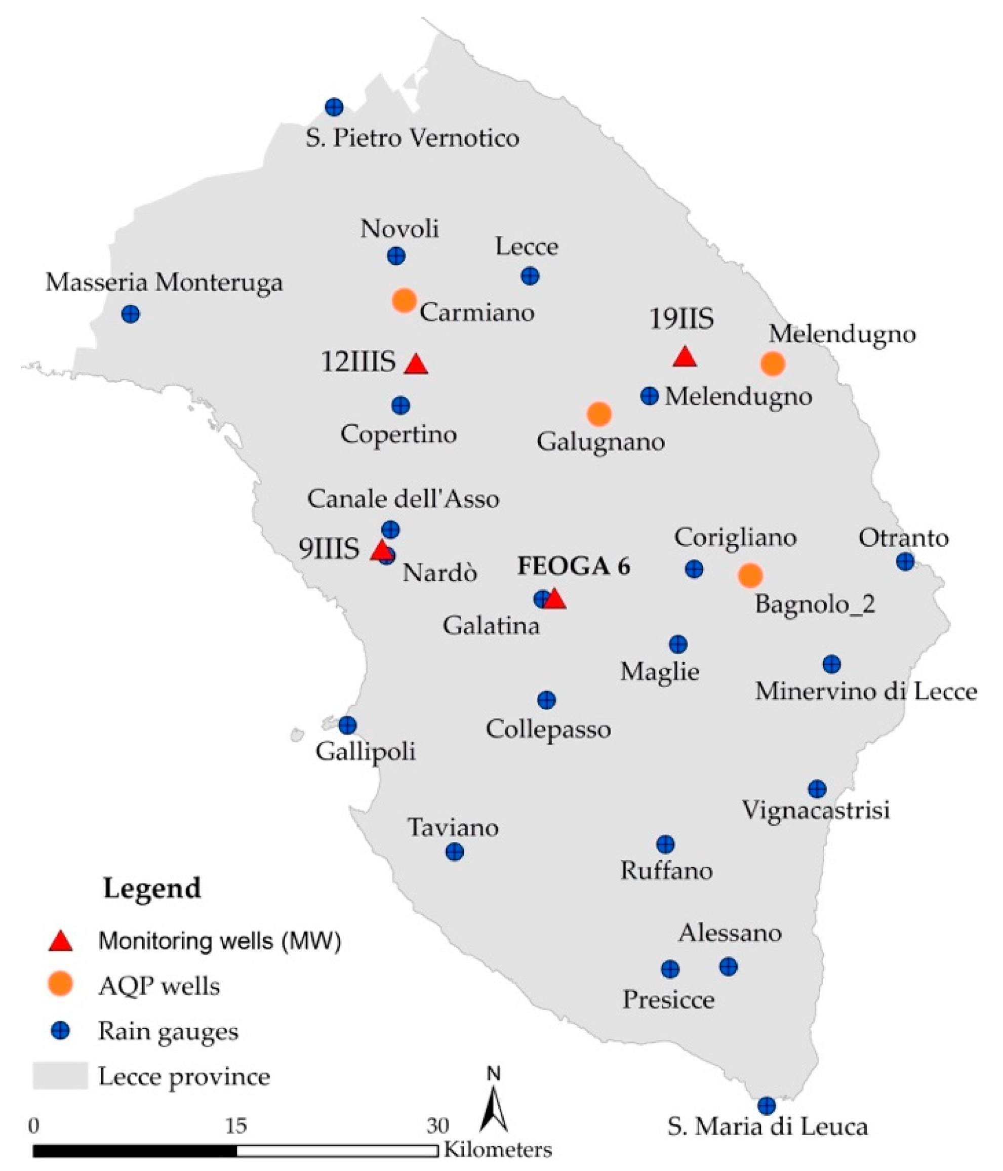
The Salento Peninsula is located in the southeastern part of Puglia region (Southern Italy) and extends from Ionian to Adriatic Sea (Figure 1). It covers 2760 km², and its limits roughly coincide with those of Lecce Province. The Salento peninsula belongs to the Apulian carbonate platform that is composed by well-bedded succession of Jurassic-Cretaceous carbonate rocks, with a thickness varying from about 3–5 km. The geological basement of the Salento Peninsula is composed by limestone and dolomitic limestone of Cretaceous age, which outcrop in large areas (Figure 1). The covers are characterized by clay, sand and calcarenite of Miocene to Pleistocene age [39]. The basement is characterized by structural highs and lows separated by sub-vertical normal, strike-slip and oblique-slip faults of Plio-Pleistocene age, striking NNW–SSE and subordinately NW–SE [40].

The Mesozoic carbonate basement represents the main deep aquifer, which is bordered by the sea. As reported by Portoghese et al. [41], precipitation in Salento is about 638 mm/year (with reference to the period 1951–2002), where 60% is lost due to evapotranspiration, 118 mm/year represent the runoff, 34 mm/year the irrigation and only 132 mm/year recharge the aquifer. Recharge is mainly of focused type because of the existence of hundreds of endorheic basins, as also occurs in the adjacent Murgia karst coastal aquifer [42]. The endorheic basins convert the internal runoff to effective infiltration, unless cascading effects between basins: considering that the surface of endorheic basins occupies more than the 40% of the total area of Salento, it is clear that they play the main role in driving both recharge and pollution transport processes. The covers may often contribute to the recharge of deep aquifer through lateral stratigraphic contacts and tectonic discontinuities. In the geological time, the Salento aquifer has been affected by vadose, water table, and transition zone karst processes, favoured by lithology and fractures under the combined effect of tectonics and glacio-eustatic oscillations [43]: thus, Salento currently shows, in addition to endorheic basins, karst plains, fracture zones, dolines, sinkholes, and karst sub-horizontal levels. These elements constitute an interconnected discontinuity system, which determines a high anisotropy of the hydraulic conductivity, with a mean high permeability at regional scale. Freshwater, with a salt content varying between 0.2 and 0.5 g/L [16], floats on saltwater of marine origin as a lens because of different density; groundwater discharges through coastal springs (sub-aerial and submarine, concentrated and diffuse), with Total Dissolved Solids (TDS) varying between 3.5 and 20 g/L. Due to the presence of low permeability carbonate units and/or tectonics dislocation of the basement, saturated zone is often found under mean sea level. However, the hydraulic continuity of the rock framework allows the development of an extensive groundwater flow system, with a consistent areal distribution of matter and heat, and hydraulic interdependence of different aquifer areas. Water levels reach maximum values of 4.5 m a.s.l. in the NW and SE sectors of the peninsula, where the maximum fresh groundwater thickness is around 120 m. The hydraulic gradient is about 0.02‰.

Taken as a whole, the aquifer represents a complex system, which combines the complexity of a tectonic karst with that of a coastal aquifer. Its detailed features are outlined in Fidelibus and Pulido-Bosch [16], who explain how the interplay of surface and subsurface features and hydrogeological coastal conditions determine from place to place different groundwater vulnerability, posing consequent different monitoring and management questions.

Starting from the 1960s, population began growing with a concurrent economic development mainly based on tourism, agriculture and small family-size manufacturing activities. Due to the high permeability of karst surface, the region cannot rely on superficial waters: thus, these changes were totally supported by the availability of groundwater, which still represents the unique water resource to satisfy drinking and, especially, irrigation demand. Starting from the 1960s, after the onset of deep drilling techniques, which allowed exploiting the carbonate karst coastal aquifer, thousands of authorized and unauthorized irrigation wells exploit groundwater. Exploitation continuously increased in the time, causing a relentless increase of salinization. Figure 2 shows the earliest distribution of irrigation, not-irrigation and urban zones for the Salento Peninsula referred to the summer season 1997 (data on land use are from SIGRIA—Information System for Water Management for Irrigation [44].

3.2. Dataset

Monthly average temperatures and rainfall data for Salento peninsula were provided by the Civil Protection of the Puglia Government [45]. Figure 3 shows the location of considered gauges, while in

Table 2. Rain gauges stations.

ID	Station Name	Latitude 1	Longitude 1	Height (m a.s.l.)
1	Copertino	40.26667	18.05000	34
2	Galatina	40.13417	18.16778	73
3	Gallipoli	40.05444	17.99444	31
4	Lecce	40.35028	18.16667	78
5	Maglie	40.10083	18.28389	77
6	Masseria Monteruga	40.33389	17.81722	72
7	Minervino di Lecce	40.08361	18.41667	98
8	Nardò	40.16694	18.03333	43
9	Novoli	40.36694	18.05056	37
10	Otranto	40.15028	18.48417	52
11	Presicce	39.88389	18.26667	114
12	Ruffano	39.96750	18.26667	125
13	S.Maria di Leuca	39.78417	18.35000	65
14	S. Pancrazio Salentino	40.41667	17.83361	62
15	S. Pietro Vernotico	40.46750	18.00083	36
16	Taviano	39.96750	18.08361	61
17	Vignacastrisi	40.00056	18.40000	94

¹ Coordinates in decimal degrees (WGS84).

their main features are summarized.

Time series of the hydrological input variables required to evaluate drought indices (Table 1) must satisfy a fundamental criterion, i.e., a record continuity not less than 30 years. From the analysis of rainfall records it emerged how the longest time window useful for the study refers to monthly rainfall in the time interval 1949–2011 only for four stations (Gallipoli, Minervino di Lecce, Nardò, and Otranto) out of the 17 located in Salento.

For temperature, instead, there are only fragmented records that prevent the analysis of drought indices that require the temperature-derived data. This is a relevant issue when dealing with all datasets, since it requires the reconstruction of missing data. However, the importance of the topic would require a proper and deep assessment of each method that is out of the scope of this paper. On this basis, we decided to use only reliable data and focus the attention on the SPI index.

Data about water level series refer to four monitoring wells (MW, location in Figure 3). As to their location, the 19IIS and 9IIIs MWs are closer to the Adriatic and Ionian coast, respectively, while the Feoga-6 and 12IIIs MWS are located between the two coasts. All belong to the northern part of the Salento aquifer. Water level series refer to historical records, which are uniquely available in the territory, adequately covering part of the period of precipitation series. Information on their location and technical features are reported in

Table 3. MW well features.

Well Name	Latitude1	Longitude1	Distance from the Closest Sea (km)	Well-head Elevation (m a.m.s.l.)	Well Depth (m a.m.s.l.)	Water Strike (m a.m.s.l.)	Static Level at Drilling (m a.m.s.l.)	Saturated Thickness ba (m) crossed by Screens ba (m)
Feoga-6	40.135	18.178	11.55	91.7	−134	−61.3	4.5	72.7
19IIS	40.293	18.299	7.5	35.7	−191.2	−179.2	3.7	12
12IIIS	40.295	18.065	14.15	42.6	−19.8	2.6	2.6	22.4
9IIIS	40.171	18.029	4.9	39.9	−29.1	1.3	1.3	30.4

¹ Coordinates in Decimal Degrees (WGS84).

. The table shows that they are of different depth; two of them have a water strike elevation below mean sea level, corresponding to the elevation of top of the carbonate basement. The saturated thickness refers to the length of well equipped with screens. During 1973–1995, water levels were measured manually with monthly frequency, with different time gaps.

Wells belong today to different public organizations: however, in the period 1973–1995 measures were carried out by operators from a same institution with similar technical means and with reference to a constant well-head having an accurate value of the elevation. Archive data do not give indications about instrumentation and type of cables. However, the accuracy in water level measures should be around 5–10 cm, which is good considering the length of cables to be used in most Salento wells. However, rather than absolute values we have considered the “variation” of water levels, which is effective even with a fair degree of accuracy. Technical sheet of drillings also report data on simple discharge tests, but little is known about the conditions of tests. Since it is not possible to check the field historical data, we generally used provided values.

Figure 3 also shows the location of four wells tapping the Salento aquifer for drinking purposes: they belong to the regional potable net (Acquedotto Pugliese, AqP). The study considers the series of chloride concentrations measured in groundwater samples drawn from these wells in pumping condition for the period 1980–2012 by AqP laboratories; data were collected with low (yearly or three-monthly) frequency in the first year (data from paper registrations) and with monthly frequency up to the end of the series.

4. Methodologies

4.1. Data Analysis

As stated in the previous paragraph, only monthly rainfall data in 1949–2011 were available for this study. Moving from some of the most recent climate studies on the Salento peninsula [46,47], we decided to investigate these time series not only in the entire interval, but also in two sub-periods, namely 1949–1979 and 1980–2011. This choice was also motivated by a visual analysis of time series and the opportunity of analysing two time series of comparable length.

Furthermore, the analysis of the rainfall dataset was also aimed at detecting the possible presence of statistically significant trends, following a practice widely diffuse in the scientific literature.

To provide a quantitative assessment of any trend in annual rainfall for the period 1949–2011, we implemented Mann–Kendall test [48,49].

Based on the null hypothesis of absence of trends, given a time series of N independent data $\underset{¯}{\mathit{x}}=[{\mathrm{x}}_1,{\mathrm{x}}_2,\dots ,{\mathrm{x}}_{\mathrm{N}}]$, this trend test relies on the computation of the following statistics:

$$\mathrm{S}={\displaystyle \sum }_{\mathrm{i}=1}^{\mathrm{N}-1}{\displaystyle \sum }_{\mathrm{j}=\mathrm{i}+1}^{\mathrm{N}}\mathrm{sgn}\left({\mathrm{x}}_{\mathrm{j}}-{\mathrm{x}}_{\mathrm{i}}\right)$$

(1)

$\mathrm{For}$$\mathrm{N}\ge 8$, statistic S can be retained asymptotically normal distributed with zero mean and variance V that, if there are ${\mathrm{t}}_{\mathrm{r}}$ ties of length r, can be expressed as [50]:

$$\mathrm{V}=\frac{\mathrm{N}\left(\mathrm{N}-1\right)\left(2\mathrm{N}+5\right)-{{\displaystyle \sum }}_{\mathrm{r}=1}^{\mathrm{N}}{\mathrm{t}}_{\mathrm{r}}\mathrm{r}\left(\mathrm{r}-1\right)\left(2\mathrm{r}+5\right)}{18}$$

(2)

According to these statements, the Mann-Kendall test is performed using the variable Z:

$$\mathrm{Z}=\{\begin{array}{cc}\frac{\mathrm{S}-1}{\sqrt{\mathrm{V}\left(\mathrm{S}\right)}}\hfill & \mathrm{S}>0\hfill \\ 0\hfill & \mathrm{S}=0\hfill \\ \frac{\mathrm{S}+1}{\sqrt{\mathrm{V}\left(\mathrm{S}\right)}}\hfill & \mathrm{S}<0\hfill \end{array}$$

(3)

which allows an easy calculation of the p-value, to be compared with the fixed level of significance. In order to take into account the effect that serial correlation can exerts on output of the test, the corrected version of the test proposed by Hamed and Rao [51] was applied.

4.2. SPI

To evaluate hydrological impacts and to explore the drought variation at inter-annual timescales, SPI was calculated aggregating monthly precipitation data over an accumulation period of 12 months [23,52]. According to McKee et al. [21], drought intensity is arbitrarily defined for values of SPI in relation to the categories shown in

Table 4. SPI drought categories ¹.

SPI Values	Drought Category
0 to −1.00	Mild drought
−1.00 to −1.50	Moderate drought
−1.50 to −2.00	Severe drought
≤−2.00	Extreme drought

¹ McKee et al. [21].

.

Afterwards, the long-term records of precipitations (X) were converted into log-normal values after removing zero values, to calculate the statistic U according to the following equation:

$$\mathrm{U}=\ln (\overline{\mathrm{X}})-\frac{{\displaystyle \sum }\ln \mathrm{X}}{\mathrm{N}}$$

(4)

where N is the number of observations.

The statistic U was then used for the calculation of two shape parameters (α and β) of the gamma distribution with:

$$\mathsf{\alpha }=\frac{\overline{\mathrm{X}}}{\mathsf{\beta }}$$

(5)

$$\mathsf{\beta }=\frac{1+\sqrt{1+\frac{4\mathrm{U}}{3}}}{4\mathrm{U}}$$

(6)

These shape parameters were then used to compute the basic equation of gamma distribution:

$$0\mathrm{G}\left(\mathrm{X}\right)=\frac{{{\displaystyle \int }}_0^{\mathrm{X}}{\mathrm{X}}^{\mathsf{\alpha }-1}{\mathrm{e}}^{-\frac{\mathrm{X}}{\mathsf{\beta }}}}{{\mathsf{\beta }}^{\mathsf{\alpha }}\Gamma \left(\mathsf{\alpha }\right)}\mathrm{dx}$$

(7)

Regarding zero observations, a new cumulative probability function was introduced

$$\mathrm{H}\left(\mathrm{X}\right)=\mathrm{q}+\left(1-\mathrm{q}\right)\mathrm{G}\left(\mathrm{X}\right)$$

(8)

where q represents the percentage of zero-values in the long-terms records of precipitations. This new probability function was transformed into a standard normal random variable with mean zero and variance of one, in which the created random variable is the value of the SPI.

The R package SPEI [24] has been used to evaluate the SPI index.

4.3. Specific Capacity and Specific Capacity Index

Well drilling technical sheets report results of discharge tests, which allow calculation of specific capacity and specific capacity index.

Specific capacity (S_c) [53] is partly a function of the aquifer transmissivity showing its same dimension (L²·T⁻¹). It is generally reported as yield per unit of drawdown:

$${\mathrm{S}}_{\mathrm{c}}=\frac{\mathrm{Q}}{{\mathrm{s}}_{\mathrm{w}}}$$

where Q is the pumping rate (L³·T⁻¹) and s_w is the drawdown (change in hydraulic head) in the well (L). Specific capacity can be normalized to aquifer thickness by using the specific-capacity index [54]:

$${\mathrm{S}}_{\mathrm{i}}=\frac{{\mathrm{S}}_{\mathrm{c}}}{{\mathrm{b}}_{\mathrm{a}}}$$

where b_a is the aquifer thickness. Specific-capacity index has the same dimension as hydraulic conductivity (L·T⁻¹). S_i is useful especially when wells do not cross all the aquifer thickness, as in the case of concerned wells. In the study S_i is calculated normalizing the specific capacity to the length of the open (uncased) borehole that intercept the saturated zone in each well as suggested by Siddiqui and Parizek [55].

S_c and S_i are used in study as “analogous” of transmissivity and hydraulic conductivity respectively, considering, with the due caution, the order of magnitude of their values for the comparison of the properties of the saturated zones intercepted by the selected wells.

5. Results

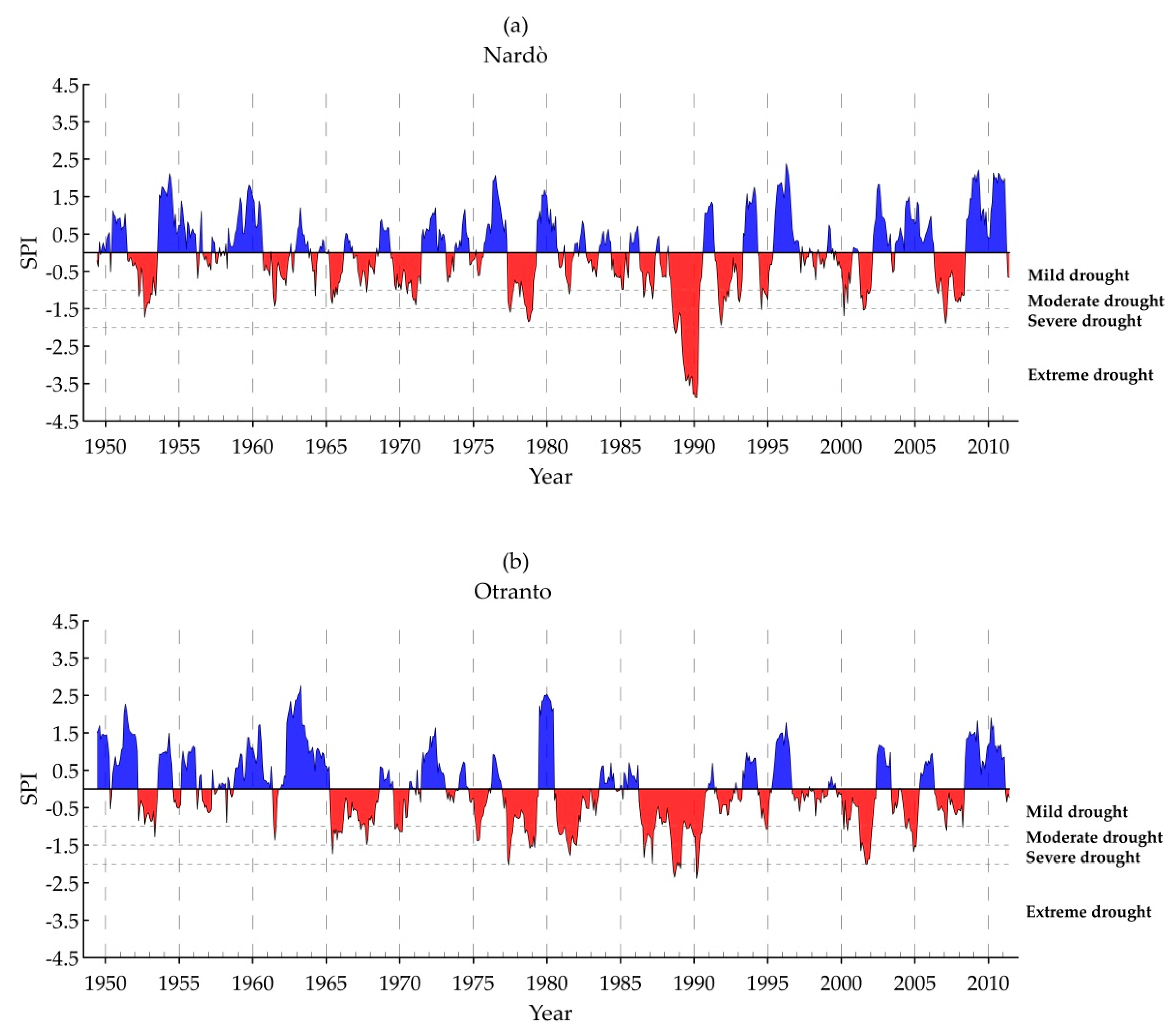
5.1. Rainfall and SPI Index Analysis

The mean values of annual rainfall for the whole time series and for the two partial sub-series, 1949–1979 and 1980–2011, are reported in

Table 5. Mean values of annual rainfall (mm).

Time Windows	Gallipoli	Minervino di Lecce	Nardò	Otranto
1949–2011	573.8	842.3	611.4	814.7
1949–1979	579.1	886.1	617.4	854.4
1980–2011	568.6	799.8	605.7	776.3

. For the sites of Gallipoli and Nardò there are no significant differences between the selected time windows; on the contrary, for Minervino di Lecce and Otranto the averages values seem showing discordances.

On the contrary, compared to the Mann–Kendall test on a yearly basis there does not seem to be a statistically significant trend at 5%. This is in agreement with the results found by D’Oria et al. [46]. It should be remarked that these usual applications of trend tests are mainly carried out with the evaluation of only type I error of the test (rejecting the null hypothesis when it is true), neglecting the type II error (non-rejecting the null hypothesis when it is false). In particular, a complete interpretation of test application needs to include the evaluation of the power of the test, whose importance was shown by several studies (e.g., [56,57,58]). However, the simple evaluation of type I error provides useful information for users.

Figure 4 shows the estimated SPI for each of the four study sites in the period 1949–2011.

As for the rainfall, the percentage of drought periods is calculated for each station with reference to both the whole period 1949–2011, and two sub-periods 1949–1979 and 1980–2011. In the first case, the percentage of droughts refers to the number of years of mild, moderate, severe and extreme droughts on the total number of values of the reference period (

Table 6. Distribution (%) of different types of droughts.

		Raingauge Stations
		Gallipoli		Minervino		Nardò		Otranto
Time Periods	1949–2011	51.14		52.35		50.20		54.77
	1949–1979	47.65		42.38		49.58		45.71
	1980–2011	54.43		61.72		50.78		63.28
		Gallipoli		Minervino		Nardò		Otranto
Time Periods		1949–1979	1980–2011	1949–1979	1980–2011	1949–1979	1980–2011	1949–1979	1980–2011
SPI Drought categories	Mild	68.60	75.12	75.16	70.89	78.21	64.62	74.55	69.55
	Moderate	18.60	11.48	16.99	13.92	17.32	19.49	20.61	19.34
	Severe	12.79	4.78	5.88	10.97	4.47	7.18	4.24	7.41
	Extreme	0.00	8.61	1.96	4.22	0.00	8.72	0.61	3.70

). This percentage is lightly greater than 50% for all stations, reaching the highest value in the station of Otranto (54.8%); the percentage for the Nardò station does not show any significant discordancy (50.2%).

Some anomalies appear considering the two sub-periods. In 1949–1979 the percentage of droughts for the Gallipoli, Minervino di Lecce and Otranto stations is lower than 50% (47.7, 42.4 and 45.7 respectively), while the percentages change abruptly in the following period, reaching values of 54.4, 61.7 and 63.3. These percentages denote an increase of drought periods between 1980 and 2011 compared to the previous 30 years. For the Nardò station, the distribution of droughts in the two sub-periods is substantially the same.

Table 6 also shows the percentage of mild, moderate, severe, and extreme droughts within the whole drought periods. From these last data an important increase of the percentage of extreme droughts clearly emerges, moving from a nearly complete lack (as for Gallipoli and Nardò) to a significant presence for all sites. The percentage of severe droughts increases as well in the second sub-period compared to the first, with the exception of Gallipoli. This station shows, in fact, a decrease in severe droughts: however, the sum of severe and extremes droughts before and after 1980 is substantially unchanged. Furthermore, for this station, a decline can also be observed for moderate droughts, in contrast to mild ones. Regarding the latter, relevant modifications affect other sites. The percentages of the extreme droughts in the other sites suggest the presence of a general shift from mild to more concentrated and heavy events (with different intensities), which is clearly shown by the drought occurred in 1989–1990.

All four sites in this two-year period showed extreme droughts during March 1989 and September–October 1990. Severe and some extreme droughts, more or less contemporaneous, occurred starting from 1978 to 1988. Other moderate to severe droughts and a few extreme droughts appear over September 2001–August 2002. Considering the SPI patterns, we selected for further analyses the period 1989–1990, being the most affected by extreme droughts within the considered time window of 1949–2011.

5.2. Drought Effects on the Salento Aquifer

The severe and extreme meteorological droughts that occurred during 1989–1990 reflect on groundwater levels measured at the Feoga-6, 12IIIS, 9IIIS and 19IIS monitoring wells (Figure 5, well locations are shown in Figure 3). Figure 5 also shows the SPI for the four rain-gauge stations for the same time window.

The largest water level measurement period (1979–1994) relates to the Feoga-6 MW. Unluckily, the available measurements of the water level were performed manually, and measures are not regularly distributed in that time. This prevents any statistical correlation between water levels and SPI values. Figure 5 allows, however, a qualitative reading of the relationships between droughts and water levels. All the water level patterns highlight a decrease of water level over the period 1989–1990, which is characterised by meteorologically severe and extreme droughts (Figure 5a). The decrease is quite abrupt for 19IIS (80 cm, between March and April 1989, Figure 5c) and 9IIIS (70 cm, between January and the end of March 1989, Figure 5d). Unfortunately, for the well 9IIIS there is a lack of measurements just in February 1989: this gap prevents a precise attribution of the onset of the water level decrease: however, both wells show a prompt response just after the extreme drought period, which starts on February 1989 and lasts till May 1989.

Well 12IIIS (Figure 5c) mimics the behaviour of 19IIS, however showing a decrease of only 15 cm between February and March 1989. The water level of the Feoga-6 MW shows a different behaviour. It shows a continuous decrease in the time, which starts from the beginning of the period of moderate and severe droughts, occurred between February and September 1987, and ending in correspondence with the termination of the period of extreme drought 1989–1990 (Figure 5b).

The increase of SPI during 1988 causes a groundwater level increase in all wells; however, the increase for the Feoga-6 is short and modest. The next increase of SPI after the end of 1990 is reflected instead in all water levels: however, even if SPI increases in 1991, showing only mild droughts and rare moderate droughts between 1992 and 1993, this does not allow the water levels to recover the values shown before 1989 for Feoga-6, 19IIS and 9IIIs. On the contrary, the water level of 12IIIS increases well beyond the previous value.

Understanding the reasons of the different behaviour of water level under the effects of droughts in the examined wells is not immediate, due to the interplay among the natural complexity of the aquifer and the human pressures on groundwater. Data on specific capacity and specific capacity index can help outlining the different hydrogeological conditions of Salento aquifer in the zones where the wells are drilled.

Table 7. Specific capacity and specific capacity index values.

Well Name	Specific Capacity Sc	Specific Capacity Index Si
	m2/s	m/s
Feoga-6	0.8 × 10−3	1 × 10−5
19IIS	2.1 × 10−3	1.8 × 10−4
12IIIS	3.7 × 10−2	1.6 × 10−4
9IIIS	6.5 × 10−2	2.1 × 10−3

shows the calculated values of S_c (m²/s) and S_i (m/s) for the four considered wells. S_c ranges from 0.8 × 10⁻³ to 6.5 × 10⁻² m²/s, while S_i varies between 1 × 10⁻⁵ and 2.1 × 10⁻³ m/s. Even if such values have to be considered only as “analogous” of transmissivity and hydraulic conductivity, respectively, having the same dimensions, they agree with literature data. As an example, mean hydraulic conductivity measured in boreholes in karst masses may range between 10⁻⁸ and 10⁻³ m/s because of the variable influence of macro-fractures and the karst network [59], while typical hydraulic conductivity of karst conduits ranges between 1 and 10 m/s.

Feoga-6 shows the lowest value of S_c, with a S_i of one or two orders of magnitude lower than the S_i of 9IIIS and 12IIIS wells. 9IIIS show the highest S_c and S_i. On the basis of these values, the reaction of MW Feoga-6 to the succession of droughts and the long time after the end of drought period before the start of water level recovering, and the length of groundwater drought (eight years) can be explained by a low transmissivity of the aquifer in the zone of the well, where groundwater circulates in a “confined” condition. The other wells promptly react to the extreme droughts, while showing a more resilient behaviour when moderate and severe droughts occur: for these wells the period of groundwater drought is lower (less than two years) than for Feoga-6 MW and the water level more rapidly recovers from the extreme drought.

In addition to the drought and the differences in the hydrological properties of the aquifer, to explain the water level variations we should also consider the role of exploitation and effective infiltration. The current and past total amounts of groundwater exploitation are not easy to assess because the official data do not include the exploitation from the thousands of abusive wells used in the irrigated areas. Since 60% of the total amount of groundwater exploitation is for irrigation [41], we will use, for the aims of the discussion, an evaluation of the total yearly amount of exploitation for irrigation referred to the entire Salento aquifer (Figure 6c) carried out by the G-Mat hydrological model [60] for the period 1970–2002 [41]. Figure 6b shows, for the same time window, the evolution of the yearly precipitation and evapotranspiration, and yearly recharge (Figure 6c) modelled with the same hydrological model [41]; groundwater stress (GWS) (Figure 6a) relates to the ratio between yearly irrigation and yearly effective infiltration [41]. Figure 6a shows the SPI values of the considered gauge stations. Figure 6d also shows groundwater chloride concentrations measured in samples from a few drinking wells located close to the considered MWs (location in Figure 3).

In correspondence with the extreme drought period of 1989–1990, recharge decreases from 54.4 to 38 mm, while irrigation increases from 44 to 61 mm (Figure 6c), causing in 1990 a GWS around 1.6 (Figure 6a). This high level of stress shows the role of exploitation for irrigation, which increases only during the low recharge periods, in worsening the effects of meteorological droughts on groundwater. The high value of GWS corresponds to a minimum for all groundwater level series of Figure 5.

Due to the coastal nature of Salento aquifer, groundwater, alongside with the decrease of water levels, shows salinization. In fact, if the reaction of inland aquifers to precipitation shortage (with a consequent recharge drought) normally consists in droughts in the different parts of the hydrogeological system, with “head drought” and “discharge and groundwater droughts” [10], in coastal aquifers a “recharge drought”, apart from varying the quantitative status of groundwater, disturbs the freshwater-seawater equilibrium as well, with a consequent worsening of its qualitative status (groundwater salinization). Figure 6d shows an increase of chloride concentrations in correspondence with the extreme drought period 1989–1990. In the following year the recharge increases, while concurrently irrigation decreases, bringing GWS back to acceptable values. However, chloride concentrations do not come back to previous levels like the water levels shown in Figure 5. Moderate-severe droughts appear between 1991 and 1992 with an increase of GWS over 0.5. The next moderate and severe drought period occurs over November 2001–August 2002, during which the GWS again increases up to 0.5 because of a new serious imbalance between recharge and irrigation.

6. Discussion

The SPI data highlight that, over 1980–2011, the percentage of drought periods increased compared to the previous 30 years; moreover, all four SPI patterns clearly denote a period of extreme droughts during March 1989 and September–October 1990. The lack of continuity in temperature series prevented the calculation of more complex indices different from the SPI. This is a precipitation-based drought index that neglects the role of temperature and evapotranspiration on drought conditions, while considering that the other variables have no temporal trend. The use of SPI data might underestimate droughts in the Apulia region in light of the trends toward warmer and marginally drier conditions during 1951–2005 [47] especially observed in the spring season series between 1961 and 2006 [61]. However, SPI data clearly allowed identifying that the worse scenery of drought in the period 1970–2010 is the period 1989–1990. Thus, the relationships between the meteorological droughts and groundwater behaviour were examined, focusing on this drought period.

The available historical data on groundwater monitoring required to this aim are of different origin and not systematic enough to allow the verification of statistical correlations. They, however, provided evidence of some significant agreements among the hydrogeological and SPI series patterns. As to groundwater levels, they do not recover pristine levels after droughts following a new phase of recharge. Actually, during the recharge periods subsequent to a drought, hydrogeological reserves should be naturally recovered. The reason of a delayed recovering of water levels may be that exploitation continues during and after the drought period at a rate that is not compatible with groundwater recovery. However, SPI indicates that other drought periods later occur, which could cause the superposition of new periods of “recharge drought” (and GW stress) on the first delayed condition of “groundwater drought”. This way, the negative effects of a succession of drought periods could not be recovered by the contribution of new volumes of effective infiltration due to the invariance of anthropic pressure. In explaining the length of “groundwater droughts”, the complexity of the karst aquifer adds to the complexity of the coupling of natural droughts and human drivers: thereby, some parts of the Salento aquifer demonstrate to be more sensitive to the succession of droughts because of their low permeability and/or transmissivity.

Concerning chloride concentrations, their evolution after the extreme drought period 1989–1990, while showing the positive effects of recharge variations, also indicates that the following moderate and severe droughts do not allow recovering the low concentrations typical of the period 1970–1989. This, with respect to water level patterns, indirectly highlights a groundwater drought period that lasts well beyond the extreme drought period 1989–1990. Data on chloride concentrations after 2002 (not shown) indicate that concentrations continue to be disturbed by the occurrence of other moderate and severe droughts (Figure 6a). Unfortunately, data from the hydrological model are based on real measurements only up to 2002, while after 2002 data are projected on the basis of downscaling the projection of climate models [41]: this prevents any further reliable comparison.

The chloride concentration patterns seem to signal that the drought period of 1989–1990 has taken groundwater in an alternative overexploited state, probably not recoverable in light of increased drought frequency and the permanent pressure of exploitation. The situation evokes the occurrence during 1989–1990 of a so-called critical transition [62], a sort of point of no return and settlement on a new equilibrium situation, however worse than the previous one.

7. Conclusions

Some conclusions can be drawn from the results.

First, the groundwater levels of all the examined wells show a decrease under the drought impact: however, the decrease is not attributable to the occurrence of droughts, but rather to the coupling of “recharge droughts” and concurrent increases of exploitation. Exploitation, indeed, increases just with water shortage, causing high GWS: this finding coincides with the conclusions of a few studies who already outlined that the primary enemy of groundwater resources is not climate change, but groundwater exploitation [63,64].

A second conclusion concerns the length of “groundwater drought” periods. The evolution of groundwater levels and chloride concentrations related to wells exploited for drinking purposes generally indicate a delay of groundwater droughts beyond the main extreme drought period of 1989–1990. In addition to the persistent pressure of the irrigation, this delay can be also linked to the superposition of different periods of “recharge drought”, which reduce water storage and prevent the water level from recovering. This means that the response of groundwater to each single drought depends on the prior state, as normally occurs in complex systems.

As a third conclusion, the study demonstrates that groundwater droughts have cascade effects on groundwater quality. Really, due to the nature of complex system and non-linear behaviour, we believe that, in the Salento coastal aquifer, the gradual change in the system drivers, such as the extreme drought period of 1989–1990, has brought groundwater to a ”tipping point” [62], which is a sort of “catastrophic bifurcation point” due to a decrease in groundwater resilience. Human drivers and climate change do not promise any future improvement: on the base of global forecasts of climate change, Portoghese et al. [41] estimate, for the next 50 years, even worse periods of GW stress in Salento, especially linked to the change of precipitation patterns, which could trigger the occurrence of other tipping points.

With all the caution due to the lack of efficient (in time and space) monitoring data, what is shown indicates that climate change, while making important changes in the relationships between all the terms of the hydrogeological balance, is not the main cause of the deterioration of the aquifer, but that the lack of control of the exploitation plays the fundamental role. Moreover, what seems clear is that groundwater responds to events in a delayed manner, moving forward the negative effects of actions (past and present).

All of the above draws attention to a significant issue concerning the methods and parameters used in environmental monitoring, which in most cases is expensive but not tuned to complex goals. The recognition of relationships among significant environmental elements requires long-term monitoring records. Unfortunately, there is a general lack of systematic studies and records that prevent catching the complexity of such relationships because monitoring mainly focuses on water quality for compliance with regulatory issues. Really, we should monitor simultaneously and in the same sites, and for consistent periods, different elements of the water cycle (drivers) and specific parameters able to describe the evolution of climate and groundwater salinization. This type of approach would provide important information about the potential non-linearity in groundwater behaviour, lag times between causes and effects, complex feedbacks and non-linear interaction between components.

References

1. European Environment Agency. Climate Change Adaptation and Disaster Risk Reduction in Europe. Enhancing Coherence of the Knowledge Base, Policies and Practices; European Environment Agency: Copenhagen, Denmark, 2017. [Google Scholar] [CrossRef]
2. Nakicenovic, N.; Swart, R. IPCC Special Report on Emissions Scenarios (SRES); Working Group III, Intergovernmental Panel on Climate Change (IPCC); Cambridge University Press: Cambridge, UK, 2000. [Google Scholar]
3. Giorgi, F.; Im, E.S.; Coppola, E.; Diffenbaugh, N.S.; Gao, X.J.; Mariotti, L.; Shi, Y. Higher Hydroclimatic Intensity with Global Warming. J. Clim. 2011, 24, 5309–5324. [Google Scholar] [CrossRef]
4. IPCC. Climate Change 2007: Impacts, Adaptation and Vulnerability; Contribution of Working Group II to the fourth Assessment Report of the Intergovernmental Panel; IPCC: Geneva, Switzerland, 2007. [Google Scholar]
5. Hiscock, K.; Sparkes, R.; Hodgson, A.; Martin, J.L.; Taniguchi, M. Evaluation of future climate change impacts in Europe on potential groundwater recharge. Geophs. Res. Abstr. 2008, 10, EGU2008-A-10211. [Google Scholar]
6. Figorito, B.; Tarantino, E.; Balacco, G.; Fratino, U. An object-based method for mapping ephemeral river areas from worldview-2 satellite data. In Remote Sensing for Agriculture, Ecosystems, and Hydrology XIV; International Society for Optics and Photonics: Edinburgh, UK, 2012; Volume 8531, p. 85310B. [Google Scholar]
7. Loukas, A.; Vasiliades, L.; Dalezios, N.R. Intercomparison of Meteorological Drought Indices for Drought Assessment and Monitoring in Greece. In Proceedings of the International Conference on Environmental Science and Technology, Lemnos Island, Greece, 8–10 September 2003; Volume B, pp. 484–491. [Google Scholar]
8. Van Loon, A.F.; Van Huijgevoort, M.H.J.; Van Lanen, H.A.J. Evaluation of drought propagation in an ensemble mean of large-scale hydrological models. Hydrol. Earth Syst. Sci. 2012, 16, 4057–4078. [Google Scholar] [CrossRef] [Green Version]
9. Chang, K.Y.; Xu, L.; Starr, G.; Paw U, K.T. A drought indicator reflecting ecosystem responses to water availability: The Normalized Ecosystem Drought Index. Agric. For. Meteorol. 2018, 250–251, 102–117. [Google Scholar] [CrossRef]
10. Wanders, N.; Van Lanen, H.A.J.; Van Loon, A.F. Indicators for Drought Characterization on a Global Scale; Watch Tech. Rep. 24; Wageningen Universiteit: Wageningen, The Netherlands, 2010. [Google Scholar]
11. Van Lanen, H.A.J.; Peters, E. Definition, Effects and Assessment of Groundwater Droughts. In Drought and Drought Mitigation in Europe Europe; Jorgen, V., Vogt, F.S., Eds.; Springer-Science+Business Media, BV: Berlin, Germany, 2000; pp. 49–61. [Google Scholar]
12. Van Loon, A.F. Hydrological drought explained. Wiley Interdiscip. Rev. Water 2015, 2, 359–392. [Google Scholar]
13. Van Loon, A.F.; Stahl, K.; Di Baldassarre, G.; Clark, J.; Rangecroft, S.; Wanders, N.; Gleeson, T.; Van Dijk, A.I.J.M.; Tallaksen, L.M.; Hannaford, J.; et al. Drought in a human-modified world: Reframing drought definitions, understanding, and analysis approaches. Hydrol. Earth Syst. Sci. 2016, 20, 3631–3650. [Google Scholar] [CrossRef] [Green Version]
14. Hughes, J.D.; Petrone, K.C.; Silberstein, R.P. Drought, Groundwater Storage and Stream Flow Decline in Southwestern Australia. Geophys. Res. Lett. 2012. [Google Scholar] [CrossRef]
15. Leduc, C.; Pulido-Bosch, A.; Remini, B.; Massuel, S. Changes in Mediterranean groundwater resources. In The Mediterranean Region under Climate Change; IRD, Ed.; IRD: Marseille, France, 2016; pp. 328–333. ISBN 978-2-7099-2219-7. [Google Scholar]
16. Fidelibus, M.D.; Pulido-Bosch, A. Groundwater temperature as an indicator of the vulnerability of Karst coastal aquifers. Geosciences 2019, 9, 23. [Google Scholar] [CrossRef] [Green Version]
17. Parisi, A.; Monno, V.; Fidelibus, M.D. Cascading vulnerability scenarios in the management of groundwater depletion and salinization in semi-arid areas. Int. J. Disaster Risk Reduct. 2018, 30, 292–305. [Google Scholar] [CrossRef]
18. Alsumaiei, A.A. Monitoring Hydrometeorological Droughts Using a Simplified Precipitation Index. Climate 2020, 8, 19. [Google Scholar] [CrossRef] [Green Version]
19. Passarella, G.; Bruno, D.; Lay-Ekuakille, A.; Maggi, S.; Masciale, R.; Zaccaria, D. Spatial and temporal classification of coastal regions using bioclimatic indices in a Mediterranean environment. Sci. Total Environ. 2019, 700, 134415. [Google Scholar] [CrossRef] [PubMed]
20. Lloyd-Hughes, B. The impracticality of a universal drought definition. Theor. Appl. Climatol. 2014, 117, 607–611. [Google Scholar] [CrossRef] [Green Version]
21. McKee, T.B.; Doesken, N.J.; Kleist, J. The relationship of drought frequency and duration to time scales. In Proceedings of the Eight Conference on Applied Climatoligy, Anaheim, CA, USA, 17–22 January 1993. [Google Scholar]
22. World Meteorological Organization. Experts Agree on a Universal Drought Index to Cope with Climate Risks; Press release No. 872; World Meteorological Organization: Geneva, Switzerland, 2009. [Google Scholar]
23. Potop, V.; Boroneanţ, C.; Možný, M.; Štěpánek, P.; Skalák, P. Observed spatiotemporal characteristics of drought on various time scales over the Czech Republic. Theor. Appl. Climatol. 2014, 115, 563–581. [Google Scholar] [CrossRef]
24. Vicente-Serrano, S.M.; Beguería, S.; López-Moreno, J.I. A multiscalar drought index sensitive to global warming: The standardized precipitation evapotranspiration index. J. Clim. 2010, 23, 1696–1718. [Google Scholar] [CrossRef] [Green Version]
25. Beguería, S.; Vicente-Serrano, S.M.; Reig, F.; Latorre, B. Standardized precipitation evapotranspiration index (SPEI) revisited: Parameter fitting, evapotranspiration models, tools, datasets and drought monitoring. Int. J. Climatol. 2013, 34, 3001–3023. [Google Scholar] [CrossRef] [Green Version]
26. Thornthwaite, C.W. An Approach toward a Rational Classification of Climate. Geogr. Rev. 1948, 38, 54–94. [Google Scholar] [CrossRef]
27. Hargreaves, G.H. Defining and using reference evapotranspiration. J. Irrig. Drain. Eng. 1994, 120, 1132–1139. [Google Scholar] [CrossRef]
28. Allen, R.G.; Pereira, L.S.; Raes, D.; Smith, M. Crop Evapotranspiration: Guidelines for Computing Crop Requirements; Irrig. Drain. Pap.; United Nations FAO: Rome, Italy, 1998; Volume 56. [Google Scholar]
29. Walter, I.A.; Allen, R.G.; Elliot, R.; Jensen, M.E.; Itenfisu, D.; Mecham, B.; Howell, T.A.; Snyder, R.; Brown, P.; Echings, S.; et al. ASCE’s standardized reference evapotranspiration equation. In Proceedings National Irrigation Symposium; Evans, R.G., Benham, B.L., Trooien, T.P., Eds.; ASAE: Phoenix, AZ, USA, 2000; pp. 209–215. [Google Scholar]
30. Droogers, P.; Allen, R.G. Estimating reference evapotranspiration under inaccurate data conditions. Irrig. Drain. Syst. 2002, 16, 33–45. [Google Scholar] [CrossRef]
31. Stagge, J.H.; Tallaksen, L.M.; Gudmundsson, L.; Van Loon, A.F.; Stahl, K. Candidate Distributions for Climatological Drought Indices (SPI and SPEI). Int. J. Climatol. 2015, 35, 4027–4040. [Google Scholar] [CrossRef]
32. Van Rooy, M.P. A Rainfall anomaly index (RAI) independent of time and space. Notos 1965, 14, 43–48. [Google Scholar]
33. Palmer, W.C. Meteorological Drought; U.S. Department of Commerce: Weather Bureau, Washington, DC, USA, 1965; Volume 45.
34. Wells, N.; Goddard, S.; Hayes, M.J. A Self-Calibrating Palmer Drought Severity Index. J. Clim. 2004, 17, 2335–2351. [Google Scholar] [CrossRef]
35. Alley, W.M. The Palmer Drought Severity Index: Limitations and assumptions. J. Clim. Appl. Meteorol. 1984, 23, 1100–1109. [Google Scholar] [CrossRef] [Green Version]
36. Mendicino, G.; Senatore, A.; Versace, P. A Groundwater Resource Index (GRI) for drought monitoring and forecasting in a mediterranean climate. J. Hydrol. 2008, 357, 282–302. [Google Scholar] [CrossRef]
37. Bloomfield, J.P.; Marchant, B.P. Analysis of groundwater drought building on the standardised precipitation index approach. Hydrol. Earth Syst. Sci. 2013, 17, 4769–4787. [Google Scholar] [CrossRef] [Green Version]
38. Wendt, D.E.; Van Loon, A.F.; Bloomfield, J.P.; Hannah, D.M. Asymmetric impact of groundwater use on groundwater droughts. Hydrol. Earth Syst. Sci. 2020. in review. [Google Scholar]
39. Ciaranfi, N.; Pieri, P.; Ricchetti, G. Note alla carta geologica delle Murge e del Salento (Puglia centro—meridionale). Mem. Della Soc. Geol. Ital. 1988, 41, 449–460. [Google Scholar]
40. Gambini, R.; Tozzi, M. Tertiary Geodynamic Evolution of the Southern Adria Microplate. Terra Nov. 1996, 8, 593–602. [Google Scholar] [CrossRef]
41. Portoghese, I.; Bruno, E.; Dumas, P.; Guyennon, N.; Hallegatte, S.; Hourcade, J.; Nassopoulos, H.; Pisacane, G.; Struglia, M.V.; Vurro, M. Impacts of Climate Change on Freshwater Bodies: Quantitative Aspects. In Advances in Global Change Research 50; Springer: Dordrecht, The Netherlands, 2013; pp. 241–304. ISBN 9789400757813. [Google Scholar]
42. Fidelibus, M.D.; Balacco, G.; Gioia, A.; Iacobellis, V.; Spilotro, G. Mass transport triggered by heavy rainfall: The role of endorheic basins and epikarst in a regional karst aquifer. Hydrol. Process. 2016, 31, 394–408. [Google Scholar] [CrossRef]
43. Canora, F.; Fidelibus, D.; Spilotro, G. Coastal and Inland Karst Morphologies Driven by Sea Level Stands: A GIS Based Method for Their Evaluation. Earth Surf. Process. Landf. 2012, 37, 1376–1386. [Google Scholar] [CrossRef]
44. INEA, Stato Dell’irrigazione in Puglia. 2000. Available online: https://sigrian.crea.gov.it/wp-content/uploads/2019/03/Irrigazione_Puglia.pdf (accessed on 11 May 2020).
45. Protezione Civile Puglia—Centro Funzionale Decentrato. Available online: https://protezionecivile.puglia.it/centro-funzionale-decentrato/ (accessed on 11 May 2020).
46. D’Oria, M.; Tanda, M.G.; Todaro, V. Assessment of local climate change: Historical trends and RCM multi-model projections over the Salento Area (Italy). Water 2018, 10, 978. [Google Scholar] [CrossRef] [Green Version]
47. Lionello, P.; Congedi, L.; Reale, M.; Scarascia, L.; Tanzarella, A. Sensitivity of typical Mediterranean crops to past and future evolution of seasonal temperature and precipitation in Apulia. Reg. Environ. Change 2013, 14, 2025–2038. [Google Scholar] [CrossRef]
48. Mann, H.B. Nonparametric Tests against Trend. Econometrica 1945, 13, 245–259. [Google Scholar] [CrossRef]
49. Kendall, M.G. Rank Correlation Methods; Griffin: London, UK, 1975; ISBN 0852641990. [Google Scholar]
50. Yue, S.; Pilon, P.; Phinney, B.; Cavadias, G. The influence of autocorrelation on the ability to detect trend in hydrological series. Hydrol. Process. 2002, 16, 1807–1829. [Google Scholar] [CrossRef]
51. Hamed, K.H.; Rao, A.R. A modified Mann-Kendall trend test for autocorrelated data. J. Hydrol. 1998, 204, 182–196. [Google Scholar] [CrossRef]
52. Tan, C.; Yang, J.; Li, M. Temporal-spatial variation of drought indicated by SPI and SPEI in Ningxia Hui Autonomous Region, China. Atmosphere 2015, 6, 1399–1421. [Google Scholar] [CrossRef] [Green Version]
53. Mace, R.E. Estimating Transmissivity Using Specific-Capacity Data; Bureau of Economic Geology, University of Texas at Austin: Austin, TX, USA, 2001. [Google Scholar]
54. Davis, S.N.; DeWiest, R.J.M. Hydrogeology; John Wiley and Sons: New York, NY, USA, 1966. [Google Scholar]
55. Siddiqui, S.H.; Parizek, R.R. Hydrogeologic Factors Influencing Well Yields in Folded and Faulted Carbonate Rocks in Central Pennsylvania. Water Resour. Res. 1971, 7, 1295–1312. [Google Scholar] [CrossRef]
56. Yue, S.; Pilon, P.; Cavadias, G. Power of the Mann-Kendall and Spearman’s rho tests for detecting monotonic trends in hydrological series. J. Hydrol. 2002, 259, 254–271. [Google Scholar] [CrossRef]
57. Vogel, R.M.; Rosner, A.; Kirshen, P.H. Brief communication: Likelihood of societal preparedness for global change: Trend detection. Nat. Hazards Earth Syst. Sci. 2013, 13, 1773–1778. [Google Scholar] [CrossRef] [Green Version]
58. Totaro, V.; Gioia, A.; Iacobellis, V. Numerical investigation on the power of parametric and nonparametric tests for trend detection in annual maximum series. Hydrol. Earth Syst. Sci. 2020, 24, 473–488. [Google Scholar] [CrossRef] [Green Version]
59. Kovács, A. Geometry and Hydraulic Parameters of Karst Aquifers: A Hydrodynamic Modeling Approach. Ph.D. Thesis, Université de Nechatel, Neuchâtel, Switzerland, 2003. [Google Scholar]
60. Portoghese, I.; Uricchio, V.; Vurro, M. A GIS tool for hydrogeological water balance evaluation on a regional scale in semi-arid environments. Comput. Geosci. 2005, 31, 15–27. [Google Scholar] [CrossRef]
61. Toreti, A.; Desiato, F.; Fioravanti, G.; Perconti, W. Seasonal Temperatures over Italy and Their Relationship with Low-Frequency Atmospheric Circulation Patterns. Clim. Chang. 2010, 99, 211–227. [Google Scholar] [CrossRef]
62. Scheffer, M. Critical Transitions in Nature and Society. Choice Rev. Online 2009. [Google Scholar] [CrossRef]
63. Ferguson, G.; Gleeson, T. Vulnerability of Coastal Aquifers to Groundwater Use and Climate Change. Nat. Clim. Chang. 2012, 2, 342–345. [Google Scholar] [CrossRef]
64. Vörösmarty, C.J.; Green, P.; Salisbury, J.; Lammers, R.B. Global Water Resources: Vulnerability from Climate Change and Population Growth Contemporary Population Relative to Demand per Discharge. Science 2000, 289, 284–288. [Google Scholar] [CrossRef] [PubMed] [Green Version]
Figure 1. Location of Salento Peninsula and schematic geological map.
Water 12 01927 g001
Figure 2. Land use map of Salento peninsula derived by SIGRIA data on land use for the summer 1997.
Water 12 01927 g002
Figure 3. Rain gauge stations (Table 2), Monitoring Wells (Table 3), and wells of the Acquedotto Pugliese (AqP) potable net considered in the study.
Water 12 01927 g003
Figure 4. SPI in the period 1949–2011, evaluated, for (a) Nardò, (b) Otranto, (c) Minervino di Lecce and (d) Gallipoli. The year marks are centred on 1 July of each year.
Water 12 01927 g004aWater 12 01927 g004b
Figure 5. SPI calculated for precipitation measured between 1979–1995 at the Nardò, Otranto, Minervino di Lecce and Gallipoli rain gauge stations (a) compared to the water level time series over 1979–1994 of the Feoga-6 (b), 12IIIS and 19IIS (c), and 9IIS (d) MWs respectively. The coloured bar covers the period 1 January 1989–31 December 1990; the date ticks are centred on 1 July of the correspondent year. The location of gauge stations and MWs is in Figure 3.
Water 12 01927 g005
Figure 6. SPI (a) calculated for precipitation measured between 1980–2002 at the Nardò, Otranto, Minervino di Lecce and Gallipoli rain gauge stations compared to (a) GWS, (b) yearly precipitation, evapotranspiration and (c) irrigation and recharge. GWS and data shown in (b) and (c) refer to the entire Salento aquifer. (d) Chloride concentrations measured in samples from AqP wells tapping groundwater for potable use. The coloured bars cover the periods 1 January 1989–31 December 1990 and November 2001–August 2002; the date ticks are centred on 1 July of the correspondent year. Location of gauge stations and AqP wells is shown in Figure 3.
Water 12 01927 g006