A Prediction Model Based on Deep Belief Network and Least Squares SVR Applied to Cross-Section Water Quality

Abstract

Recently, the quality of fresh water resources is threatened by numerous pollutants. Prediction of water quality is an important tool for controlling and reducing water pollution. By employing superior big data processing ability of deep learning it is possible to improve the accuracy of prediction. This paper proposes a method for predicting water quality based on the deep belief network (DBN) model. First, the particle swarm optimization (PSO) algorithm is used to optimize the network parameters of the deep belief network, which is to extract feature vectors of water quality time series data at multiple scales. Then, combined with the least squares support vector regression (LSSVR) machine which is taken as the top prediction layer of the model, a new water quality prediction model referred to as PSO-DBN-LSSVR is put forward. The developed model is valued in terms of the mean absolute error (MAE), the mean absolute percentage error (MAPE), the root mean square error (RMSE), and the coefficient of determination ($R^2$). Results illustrate that the model proposed in this paper can accurately predict water quality parameters and better robustness of water quality parameters compared with the traditional back propagation (BP) neural network, LSSVR, the DBN neural network, and the DBN-LSSVR combined model.

1. Introduction

Rapid population growth, industrialization, and the use of fertilizers and pesticides for agricultural purposes have made the water environment problem increasingly serious [1,2]. Therefore, predicting water quality parameters is of great significance for the control of water pollution. At present, water quality prediction models mainly include mechanism water quality prediction models and non-mechanism water quality prediction models. The mechanism water quality prediction model is relatively complicated, using the system structure data to simulate water quality, which is constrained by the internal and external environment of the water body, but it is more versatile and applicable to any water body. The earliest water quality simulation model is the Streeter–Phelos (S–P) model that belongs to the one-dimensional steady-state oxygen balance model, having been widely used so far, and then derived the BDO-DO bilinear coupling system model [3]. Subsequently, Occident has developed a variety of water quality models, such as the QUAL model [4] and the WASP model [5], which has been widely used in the simulation of river water quality. In 1992, Warren [6] proposed to take advantage of MIKE21 for a modeling system for estuaries, coastal waters, and seas. Hayes [7] coupled a quasi-static two-dimensional dissolved oxygen reservoir model (DORM-II) and a daily scale optimal dispatch model in the Cumberland watershed to improve downstream water quality. A two-dimensional (2D) numerical simulation model was established for the water environment of the Mudan River using hydrodynamic and water quality model based on EFDC [8]. However, these water quality simulation models need to consider the influence of physical, chemical, biological, and other external environments on the water body, so the modeling is complicated.

While, non-mechanism water quality prediction model is a data-driven model, a “black box” method, and established by statistical methods or other mathematical methods, having the higher popularity in that the output is fast and the calculation process does not need to consider the physical mechanism of the research object [9]. The existing non-mechanism water quality prediction methods mainly include the regression fitting method, the time series method, the gray theory method, and the artificial neural network (ANN), and so on. In 1971, a mathematical model was established, taking advantage of mathematical statistics to predict river water quality, focusing on the “black box” method without involving chemical, biological, and physical relationships [10]. Hu et al. [11] proposed Grey Relational Analysis (GRA) based on the distance between points and intervals to predict water quality, but the data calculation is more complicated. Batur et al. [12] made use of multivariate statistical methods, cluster analysis (CA), and principal component analysis (PCA) to predict the water quality of Manchar Lake (Pakistan), whose result was considerable. Jaloree et al. [13] used a decision tree model to predict the water quality of the Narmada River in 2014, involving five water quality indicators. The deep Bi-S-SRU (Bi-directional Stacked Simple Recurrent Unit) learning network is proposed, in order to frame-accurate prediction scheme of water quality in smart mariculture [14]. In [15], the author established a water quality prediction model for four parameters, dissolved oxygen, chlorophyll, conductivity, and turbidity, using ANN. The ANN and decision tree algorithm were combined to predict the water quality of China’s Chaohu Lake in [16], in this study, multiple variables of water quality data were processed, and better prediction results were obtained. In condition, in [17], a new hybrid method was developed, using artificial neural network and Markov chain method to predict dissolved oxygen (DO) which is the main indicator of water quality [18]. Yan et al. [19] proposed a genetic algorithm (GA) and particle swarm optimization (PSO) algorithm to optimize the back propagation (BP) neural network to predict the biochemical oxygen demand of the lake, moreover, the forecast accuracy has been greatly improved. A affinity propagation clustering method based on a least squares support vector machine (AP-LSSVM) was put forward for water quality prediction, which is a supervised learning method, but it is more sensitive to vacancies [20]. Solanki et al. [21] applied the deep belief network model in 2015 to analyze and predict the chemical eigenvalues of water, especially DO and pH, their research indicates that deep learning techniques can provide more accurate results than supervised learning-based techniques. Deep learning methods have achieved great application results in the fields of image classification [22], speech recognition [23], fault diagnosis [24], and prediction estimation [25] due to the powerful big data processing ability and classification capability. For instance, a deep belief network (DBN), one of the commonly used neural networks in deep learning, is used to classify spectral images by extracting hyperspectral features [26], identify and classify different discharge patterns [27], and predict traffic flow [28,29] and weather [30]. It has been verified that deep learning methods are better than traditional methods. Besides, Marir et al. [31] developed a model to discover the abnormal behavior from large-scale network traffic data using a combination of deep feature extraction and multi-layer ensemble support vector machines (SVMs) in a distributed way. Fadlullah et al. [32] envisaged a reward-based deep learning structure, which jointly employs a deep convolutional neural network (CNN) and a deep belief network (DBN) to predict the traffic load value matrix and construct the final action matrix.

In this paper, we proposed a new deep learning method that combines DBN neural network optimized by PSO with least squares support vector regression (LSSVR) to predict water quality parameters. Then, the BP, DBN, LSSVR, and DBN-LSSVR methods were used as comparative experiments, and we evaluate the performance of each method. Experimental results demonstrate that the method proposed in this paper has a higher accuracy of prediction than the other four methods.

2. Materials and Methodology

2.1. Study Area and Monitoring Data

In this paper, the water quality data of Sanhe East Bridge, a control section of Juhe River on the Haihe River Basin, is selected as the research object. It is located in Sanhe City (39°48′ N–40°05′ N, 116°45′ E–117°15′ E), in Hebei Province of China, belonging to a temperate continental monsoon climate with distinct seasons throughout the year. The landform types are complex, with low hills, plains, and depressions. The Juhe River is one of the important river systems on the Haihe River Basin, which flows through three provinces of Hebei, Beijing, and Tianjin, with a total length of 206 km, a drainage area of 2276 km, and an annual runoff of 29.09 million cubic meters. There are important tributary rivers: Jinji River, Zhouhe River, and Huanxiang River.

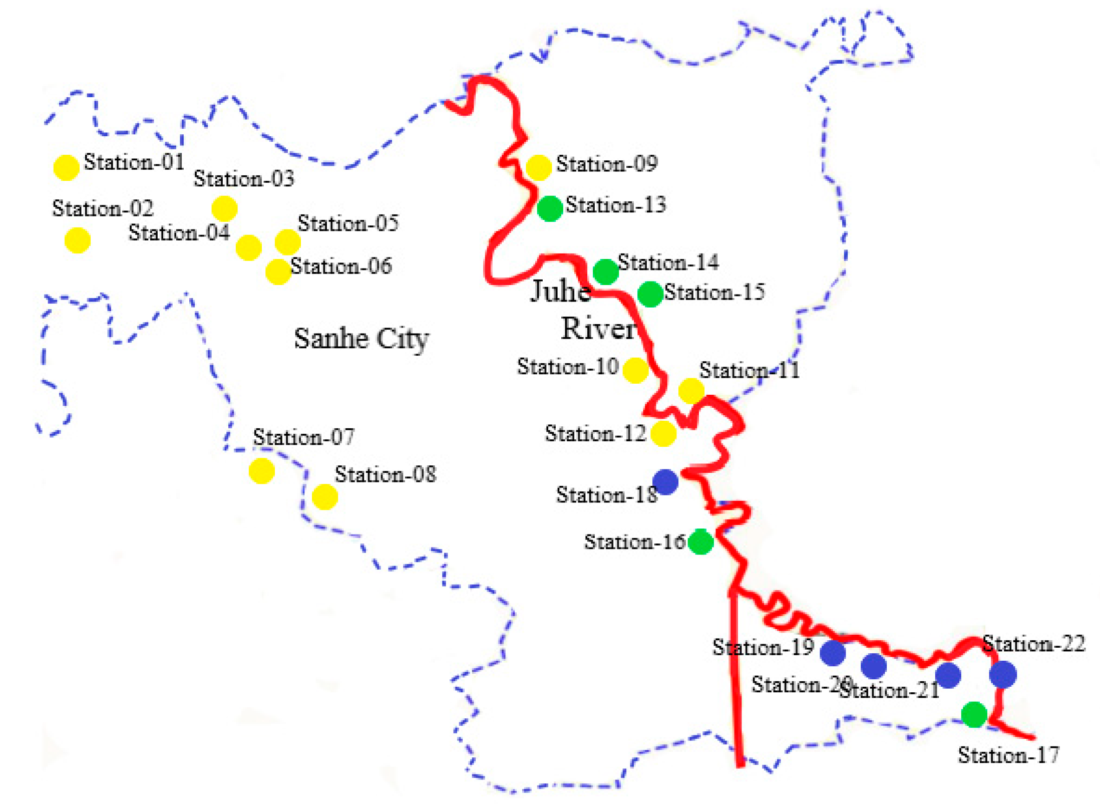
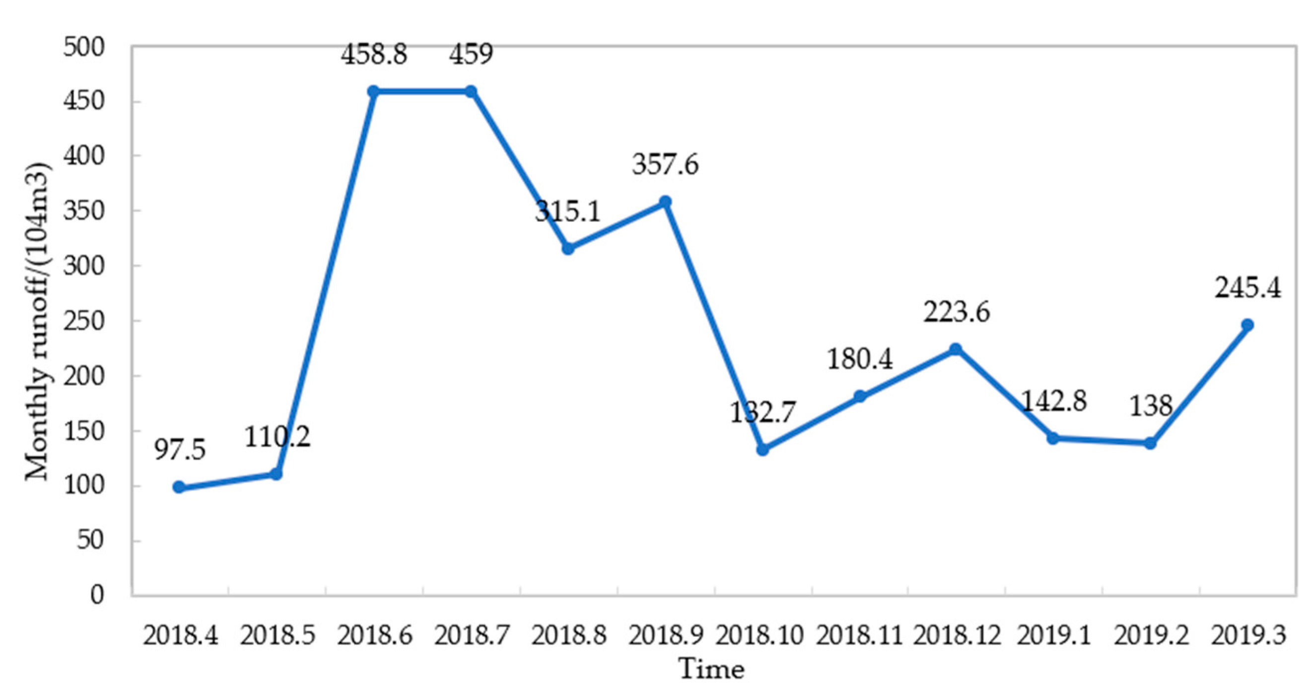
Human activities mainly include industrial wastewater pollution, domestic sewage pollution, livestock and poultry farming wastewater pollution, and garbage pollution, which has caused critical environmental pressure on the water quality of the Juhe River. In addition, as a pilot zone of China’s free trade, Hebei’s rapid economic development has also lead to serious pollution of the water quality of the Juhe River. The experimental data in this paper is monitored by the Langfang Environmental Monitoring Station, which is from the Beijing Environmental Planning Institute of the Ministry of Environmental Protection. Figure 1 is the monitoring station map of the Juhe River. Figure 2 shows the annual runoff of the Juhe River during our analyzed period, which is real-time monitoring data transmitted from the monitoring system of Sanhe Hydrological Station by wireless communication.

Figure 1. Location of the monitoring stations on the Juhe River.

Figure 2. Annual runoff of the Juhe River.

The summer and early autumn of the study area are seasons with relatively concentrated rainfall in that it is easily controlled by the southeast warm and humid airflow, besides, according to the quality of the data provided by the organization, so the time interval of data in this paper is from 18 August 2018, to 18 March 2019, collected by every four hours, a total of 1086 data.

In Figure 1, there are 22 monitoring stations. The stations marked in green are the stations for the construction of sewage villages along the banks of the river, the yellow are the stations with more pollution on the Juhe River, and the blue are the stations in the buffer zone of the provincial boundary, which require higher water quality and is greatly affected by upstream water quality.

2.2. Feature Extraction Based on DBN Model

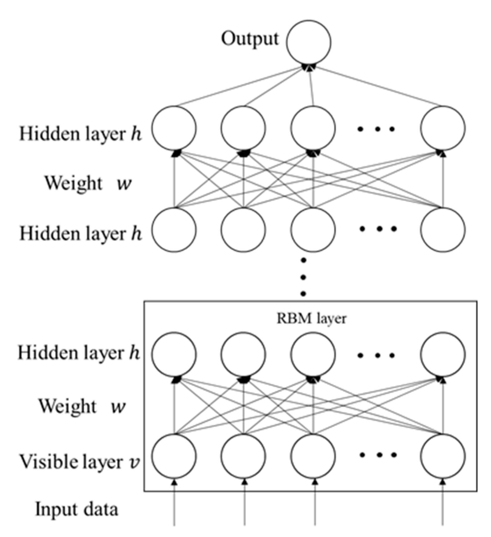
DBN is an important model in deep learning [33]. It is a probabilistic generative model composed of a series of Restricted Boltzmann Machine (RBM) units [34]. There is no connection between each neural unit in each layer of the RBM model, furthermore, each neural unit in the visible layer is connected to each neural unit in the hidden layer. Also, the output of each layer of RBM is used as the input of the next layer. Its structure is shown in Figure 3.

Figure 3. Deep belief network (DBN) model architecture.

The bottom layer of the DBN model adopts a multi-layer RBM structure. The greedy algorithm is used to train the sample data layer by layer. The parameters obtained by training the first layer RBM are used as the input of the second layer RBM, and the parameters of each layer are obtained by analogy. The training process belongs to unsupervised learning. The joint configuration energy of the visible layer and the hidden layer in RBM can be expressed as the following:

$$E\left(\nu ,h|\theta \right)=-{\displaystyle \sum }_{i=1}^n{a}_i{v}_i-{\displaystyle \sum }_{j=1}^m{b}_i{h}_i-{\displaystyle \sum }_{i=1}^n{\displaystyle \sum }_{j=1}^m{v}_i{w}_{ij}{h}_j$$

(1)

where, $\theta =\{w_{i\dot{j}},a_i,b_j\}$, it is the connection weight value between visible unit $i$ and hidden unit$j$, $a_i$ is an internal bias of visible layer neurons, and$b_j$ is hidden layers.

When the parameter $\theta$ is fixed, based on the energy function, the joint probability distribution of the visible layer and the hidden layer can be obtained Equation (2) and combining it with Equation (3) as follows:

$$P\left(\nu ,h|\theta \right)=\frac{e^{-E\left(v,h|\theta \right)}}{Z^{\theta }}$$

(2)

$$Z^{\theta }={\displaystyle \sum }_{v,h}{e}^{-E\left(v,h|\theta \right)}$$

(3)

When the state of the visible layer $\nu$ is known, the activation probability of the $j$th neural unit of the hidden layer $h$ is obtained:

$$P\left(h_j=1|\nu ,\theta \right)=\sigma \left( b_j+{\displaystyle \sum }_i{v}_i{w}_{ij}\right)$$

(4)

When the hidden layer state $h$ is known, the activation probability of the $i$th neural unit of the visible layer $\nu$ is obtained:

$$P\left(v_i=1|h,\theta \right)=\sigma \left( a_i+{\displaystyle \sum }_i{h}_i{w}_{ij}\right)$$

(5)

where, $\sigma \left(x\right)$=$\frac{1}{1+\exp \left(-x\right)}$ is an activation function, named the sigmoid function. Each neuron will determine its state value as 1 or 0 with probability$P$.

In the unsupervised learning process, the purpose of training RBM is to obtain the model parameters, which can be given by the log-likelihood function as follows:

$$L\left(\theta \right)={\displaystyle \sum }_{n=1}^{N}ln\left(v^n,h\right)$$

(6)

$$\theta =argmaxL\left(\theta \right)=argmax{\displaystyle \sum }_{n=1}^{N}ln\left(v^n,h\right)$$

(7)

In the training process, due to the complex calculation of the normalization factor $Z^{\theta }$, it is generally approximated by sampling methods such as Gibbs [33]. Hinton [35] proposed a comparative diversification (CD) rapid learning algorithm to train network parameters, thereby improving training efficiency.

In this paper, in order to mine the essential features of the water quality of the cross-section, the DBN network is used to extract the features of the water quality. At the top level of the model, the LSSVR layer is used to optimize the prediction results, afterward, the abstract features obtained by the training and learning of the bottom model are used as the input of the LSSVR layer, furthermore, the prediction results are output through the LSSVR layer fitting. At the same time, the LSSVR layer is also required to fine-tune and optimize the obtained model parameters. This process is supervised learning.

2.3. Optimizing DBN Model Using PSO

Particle Swarm Optimization (PSO) is an evolutionary computing technology developed by Kennedy and Eberhart, in 1995, whose idea stems from the study of bird predation behavior [36]. The particle swarm algorithm first generates a random solution, and then iteratively finds the optimal solution with the best fitness value. This algorithm has been widely applied in the field of optimization methods with the advantages of simple and easy implementation, less setting parameters, and fast convergence speed, etc.

The basic form of particle swarm optimization algorithm is composed of a group of particles, each particle determines its flight direction through the value and speed of the adaptive function, gradually moving to a better area, and finally searching for the global optimal solution. The position of the particle represents the candidate solution to the problem sought, corresponding to the weight value in the neural network.

To optimize the problem, the position, velocity, and fitness value of each particle are determined by the following mathematical Equation (8) and combining it with Equation (9):

$$V_i\left[k+1\right]=w{V}_i\left[k\right]+c_{1}ran{d}_1\left(p_{ibest}-P_i\left(k\right)\right)+c_{2}ran{d}_2\left(g_{ibest}-P_i\left(k\right)\right)$$

(8)

$$P_i\left(k+1\right)=P_i\left(k\right)+V_i\left[k+1\right]$$

(9)

where, $V_i$ is the velocity of the particle, $P_i$ is the current position of the particle, i = 1, 2,$\cdots$n, n replaces the total number of particles in the particle group; k represents epoch; rand is a random number between (0,1) to increase the randomness of the search; $\omega$ is the inertial weight, adjusting the search range, which is a non-negative number;$c_1$ and $c_2$ are acceleration constants that play the role of adjusting the maximum learning step; pbest is the personal optimal value and gbest is the global optimal value.

The particle swarm optimization algorithm procedures are usually illustrated as follows:

Step 1: Initial

Initialize the particle population where the population size is n, including random position and velocity.

Step 2: Evaluation

According to the fitness function, the fitness of each particle is evaluated.

Step 3: Find the Pbest

For each particle, comparing its current fitness value with the fitness value corresponding to the individual’s historical best position (pbest), the current best position pbest will be updated with the current position if the current fitness value is higher.

Step 4: Find the Gbest

For each particle, comparing its current fitness value with the fitness value corresponding to the global best position (gbest), the global best position gbest will be updated with the current particle position if the current fitness value is higher.

Step 5: Update the Velocity

Update the speed and position of each particle according to Equations (8) and (9).

Step 6: Algorithm Over

The particle swarm optimization algorithm is judged by the end condition. According to the set end condition of the algorithm, which is the maximum number of iterations or the target fitness value, if the condition is not met, then jump to step 2, otherwise, the global optimal value gbest is output.

2.4. Least Squares Support Vector Regression Machine

The least squares support vector regression machine is a machine learning method based on statistical theory and structural risk minimization criterion. Different from the support vector regression machine, LSSVR replaces inequality constraints by equality constraints, using the loss function and error square as the empirical loss of the training set, and transforming solving quadratic programming problems into solving linear equations, which can effectively improve the calculation speed and convergence accuracy, and has a good promotion performance. The training of the LSSVR model is to supervised train the model through input values and label values, and update the parameters of the model. Its specific form is as follows:

$$minJ\left(\omega ,\xi \right)=\frac{1}{2}{\omega }^T\omega +\frac{C}{2}{\displaystyle \sum }_{i=1}^l{\xi }^T\xi$$

(10)

$$s.t.y_i={\omega }^T\phi \left(x_i\right)+\mu +{\xi }_i \left(i=1,2,\cdots ,l\right)$$

(11)

where, $x_i$∈$R^l$ is the input vector, $y_i$∈$R^l$ is the output vector, $\omega$ is a weight vector and C∈$R^{+}$ is a regularization parameter, which is an empirical parameter set manually, ${\xi }_i$∈R, $s.t.$, and $\mu$ represent restrictions, empirical error, and bias, respectively. $\phi \left(·\right)$ is the kernel function, which is the nonlinear mapping of the input space to the feature space. Here, we choose to use the RBF radial basis kernel function. To solve the above-constrained optimization problem, the Lagrange polynomial function of the dual problem has the following form:

$$L\left(\omega ,\mu ,\xi ,\eta \right)=J\left(\omega ,\xi \right)-{\displaystyle \sum }_{i=1}^l{\eta }_i\left({\omega }^T\phi \left(x_i\right)+\mu +{\xi }_i-y_i\right)$$

(12)

where $\eta$ = [${\eta }_1,{\eta }_2,{\eta }_i,\cdots {\eta }_l$], on behalf of the Lagrange multiplier. According to the Karush–Kuhn–Tucher (KKT) condition, find the partial derivatives of$\omega ,\mu ,{\xi }_i,{\eta }_i$, respectively, and eliminate $\omega ,{\xi }_i$, then the following linear Equation (13) can be obtained:

$$\left[\begin{array}{cc}0& I^T\\ I& \Psi +C^{-1}E\end{array}\right]\times \left[\begin{array}{c}\mu \\ \eta \end{array}\right]=\left[\begin{array}{c}0\\ y\end{array}\right]$$

(13)

where I = ${\left[1,1,\cdots ,1\right]}^T$, ${\Psi }_{ij}$ is the kernel function K($x_i,y_i$) that satisfies the Mercer condition, E is the unit matrix of $l\times l$ dimension, y = ${\left[y_1,y_2,\cdots ,y_l\right]}^T$, while the mathematical model of the least squares support vector regression machine can be obtained as follows:

$$y=f\left(x,\eta \right)={\displaystyle \sum }_{i=1}^l{\eta }_{i}k\left(x,x^i\right)+\mu$$

(14)

2.5. Prediction Model Based on PSO Optimized DBN Network and LSSVR

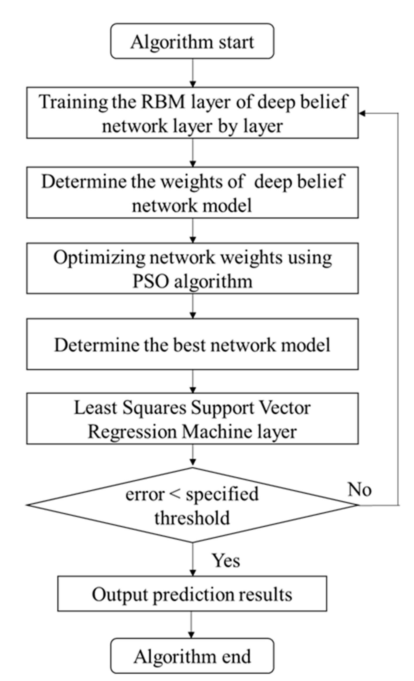
The prediction model constructed in this paper uses deep learning as the pre-processing system of the least squares support vector regression machine. Different from other water quality prediction methods, the deep belief network is used here to fully excavate the essential characteristics of the water quality of the cross-section, rather than as a prediction network, for instance, a single BP network or DBN network is adopted to predict water quality directly. Firstly, apply DBN to perform feature learning on the original water quality data to extract essential feature information that reflects the water quality change trend. Then, utilize the PSO optimization algorithm to solve the optimal initial weight value of the DBN network model. The DBN-LSSVR model is used as the prediction model after the DBN model feature extraction, that is, based on the feature vector output from the DBN model, we optimize and train the least square support vector regression machine, then establish water quality prediction model depended on the optimal combination of LSSVR model parameters and kernel function parameters in this paper. The specific algorithm steps of the model are as follows:

Step 1:

Determination of DBN model parameters. Initialize the learning rate and the number of iterations. The number of visible layer neurons is determined by the number of input features and the number of hidden layer neurons and the number of hidden layers, as well as the weights and thresholds of each layer, are determined in the training RBM layer by layer. Next, use the CD algorithm to pre-train each layer of RBM, while, regard the output of each lower layer RBM as the input of the higher layer RBM, and then train the higher layer RBM. The data will undergo feature extraction and reduce the dimension, output the feature vector, and obtain the appropriate initial weight of the model after each layer of RBM training. This step is mainly to pre-train each RBM layer of the DBN model.

Step 2:

To overcome the shortcoming that the DBN network is easy to fall into local optimum during the learning and training process, utilize the PSO optimization algorithm to dynamically optimize and adjust all RBM model parameters, and find the optimal initial weight of the network model.

Step 3:

Determination of LSSVR model parameters. The output of the top-level RBM is used as the input of the LSSVR regression layer to train the LLSVR regression model. When the maximum number of cycles or the error is less than the specified threshold, the LSSVR model training is ended, and the LSSVR prediction model is constructed with the optimal combination parameters.

Step 4:

After the LSSVR model training is completed, each layer of the RBM network can only ensure that the weights in its own layer are optimal for the feature vector mapping of this layer, not for the feature vector mapping of the entire DBN and LSSVR combined model. So it is necessary that the top-level LSSVR model propagates from top to bottom to each layer of RBM, and iteratively updates the weights and offsets of the fine-tuned DBN network until the model converges, and the training of the model is completed.

The following Figure 4 is the flow chart of the combined prediction model.

Figure 4. Particle swarm optimization-DBN-least squares support vector regression (PSO-DBN-LSSVR) prediction model flow chart.

2.6. Evaluation of Performance

In this paper, the data set is divided into two subsets for training and testing the model, the first 80% of the data set is used for the training set, and the remaining 20% is used for testing the model. To evaluate the performance of the PSO-DBN-LSSVR model and other prediction models, the following model prediction effect evaluation indicators are applied, while the calculation formulas are as follows:

$$MAE=\frac{1}{n}{\displaystyle \sum }_{i=1}^n\left|y_i-\widehat{y_i}\right|$$

(15)

$$MAPE=\frac{1}{n}{\displaystyle \sum }_{i=1}^n\frac{\left|y_i-\widehat{y_i}\right|}{y_i}\times 100$$

(16)

$$RMSE=\sqrt{\frac{1}{n}{\displaystyle \sum }_{i=1}^n{\left(y_i-\widehat{y_i}\right)}^2}$$

(17)

$$R^2=\frac{{\left({{\displaystyle \sum }}_{i=1}^n\left(y_i-\overline{y_i}\right)\left(\widehat{y_i}-\overline{\widehat{y_i}}\right)\right)}^2}{{{\displaystyle \sum }}_{i=1}^n{\left(y_i-\overline{y_i}\right)}^2{{\displaystyle \sum }}_{i=1}^n{\left(\widehat{y_i}-\overline{\widehat{y_i}}\right)}^2}$$

(18)

where MAE is the mean absolute error, MAPE is the mean absolute percentage error, RMSE is the root mean square error, and $R^2$ is the coefficient of determination. In Equations (15)–(18), n is the number of prediction points, $y_i$ represents the true value of the water quality parameter at the ith prediction point, $\overline{y_i}$ is the average value of the true value of the water quality parameter at the ith prediction point, $\widehat{y_i}$ is the predicted value of the ith prediction point model, $\overline{\widehat{y_i}}$ is the average value of the predicted value of the ith prediction point water quality parameter model.

3. Results and Discussion

3.1. Data Selection and Preprocessing

The experimental data is collected by the environmental monitoring station every four hours, by means of the IoT system, using the water quality data acquisition module for the data acquisition, the transmission module for the data transmission, and the cloud server module for the cloud storage of the data. We selected 9 chemical factors, including water temperature (T, °C), pH, dissolved oxygen (DO, mg/L), conductivity (μS/cm), turbidity (NTU), potassium permanganate index (COD, mg/L), total phosphorus (TP, mg/L), and ammonia nitrogen (NH₄N, mg/L). It is critical that these parameters are important parameters for evaluating water quality and directly related to the prediction of water quality. We used the first eight chemical factors as the input characteristic parameters, and total nitrogen as the output parameter, which is also the water quality parameter to be predicted in this paper. We selected the first 870 data of the cross-sectional water quality as the training set and the last 216 data as the test set to predict the water total nitrogen content.

Besides, the reason that the tested water quality parameters come from different Internet of Things (IoT) collection devices, equipment errors or faults, and human factors will cause the lack or abnormality of the collected water quality data. Therefore, before the construction of a deep learning network, it is essential to complete and correct the dataset [37]. The average method and k nearest neighbor (KNN) completion algorithm are more commonly data completion methods, so the KNN completion algorithm is used to complete and correct the collected data in this paper. The main principle of KNN is to select the k nearest samples of missing data according to the characteristics of high similarity between adjacent data and regard their average value as the missing data, where the Euclidean distance is used to judge the distance between sample points, the formula is as follows:

$$d\left(X_i,X_i\right)=\sqrt{{\displaystyle \sum }_{r=1}^m{\left(x_{ir}-x_{jr}\right)}^2}$$

(19)

where, $X_i=\left\{x_{i1},x_{i2},\cdots ,x_{im}\right\}$, replaces the first m-dimensional data of the ith sample, $x_{ir}$ is the rth attribute of the ith sample.

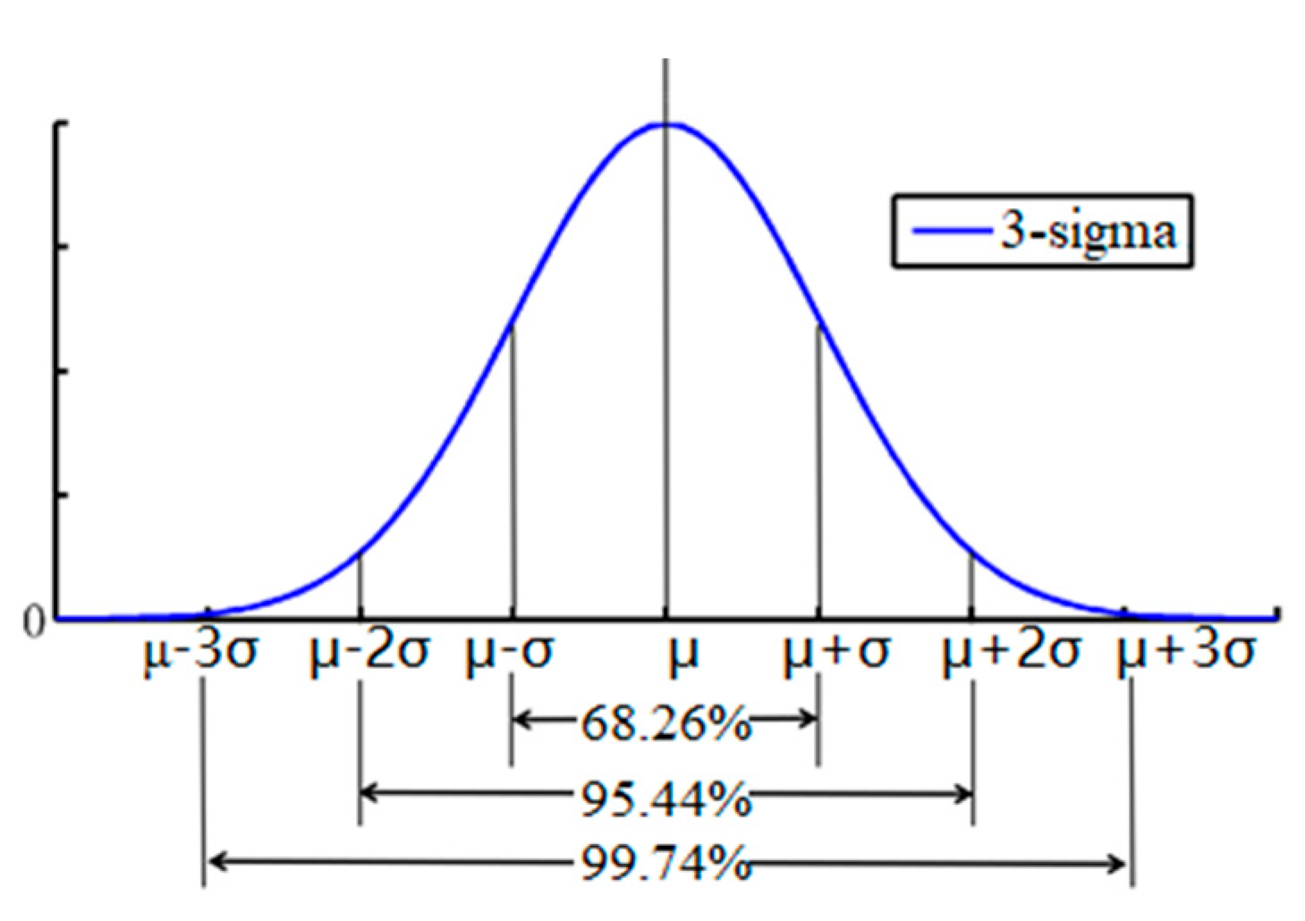
After completing the missing data, adopt the Pauta Criterion to eliminate the abnormal data in the sample data. The formula is as follows and the Pauta Criterion can be described in Figure 5.

$$\Delta x_i>3\sigma$$

(20)

where, $\Delta x_i=x_i-\overline{x_i},$ $\sigma =\sqrt{\frac{{{\displaystyle \sum }}_{i=1}^n\Delta x_i}{n-1}}$, when the above formula holds, it is determined as abnormal data.

Figure 5. Pauta Criterion.

where, $\tilde{x}$(i) is the normalized data value, $x\left(i\right)$ is the input data, $x_{max}$ and $x_{min}$ are the maximum and minimum values of the input data, respectively.

There are a total of 1086 experimental data, and the missing data accounts for about 3%, which is complemented by the k nearest neighbor completion algorithm. Abnormal data accounted for about 5%. After using the Pauta Criterion to eliminate abnormal data, the k nearest neighbor completion algorithm is also used to correct the data.

3.2. Results of Experiments

The algorithm is implemented using the matlab2018a experimental simulation platform, and the prediction model simulation program is written to predict the total nitrogen content. In this paper, five prediction models, BP, LSSVR, DBN, DBN-LSSVR, and PSO-DBN-LSSVR, are established respectively, and the prediction performance is compared.

Establish prediction models for water quality time series. For the BP prediction model, the structural parameter is 8-13-1, where the number of input layer neurons is 8, the number of hidden layer neurons is 13, the number of output layer neurons is 1, the learning rate is 0.001, the learning target is 0.01, and iterate 3000 times. The learning parameters C and δ of the LSSVR model are optimized and selected by the grid search method, and the iteration step is 1. We establish a double hidden layer DBN network structure composed of RBM1 and RBM2, it is found that the structural parameter of 8-12-4-1 is the best after many iteration experiments, where the number of visible layer neurons is 8, the number of RBM1 hidden layer neurons is 12, the number of RBM2 hidden layer neurons is 4, and the LSSVR output layer is 1. The RBM learning rate is set to 0.05, the number of iterations is 3000, and the population size is set to 50 in the PSO algorithm. After many experiments, it is found that the optimal parameter combination of LSSVR is C = 96 and δ = 1.5, then utilized the optimal prediction model to predict the total nitrogen (TN) content.

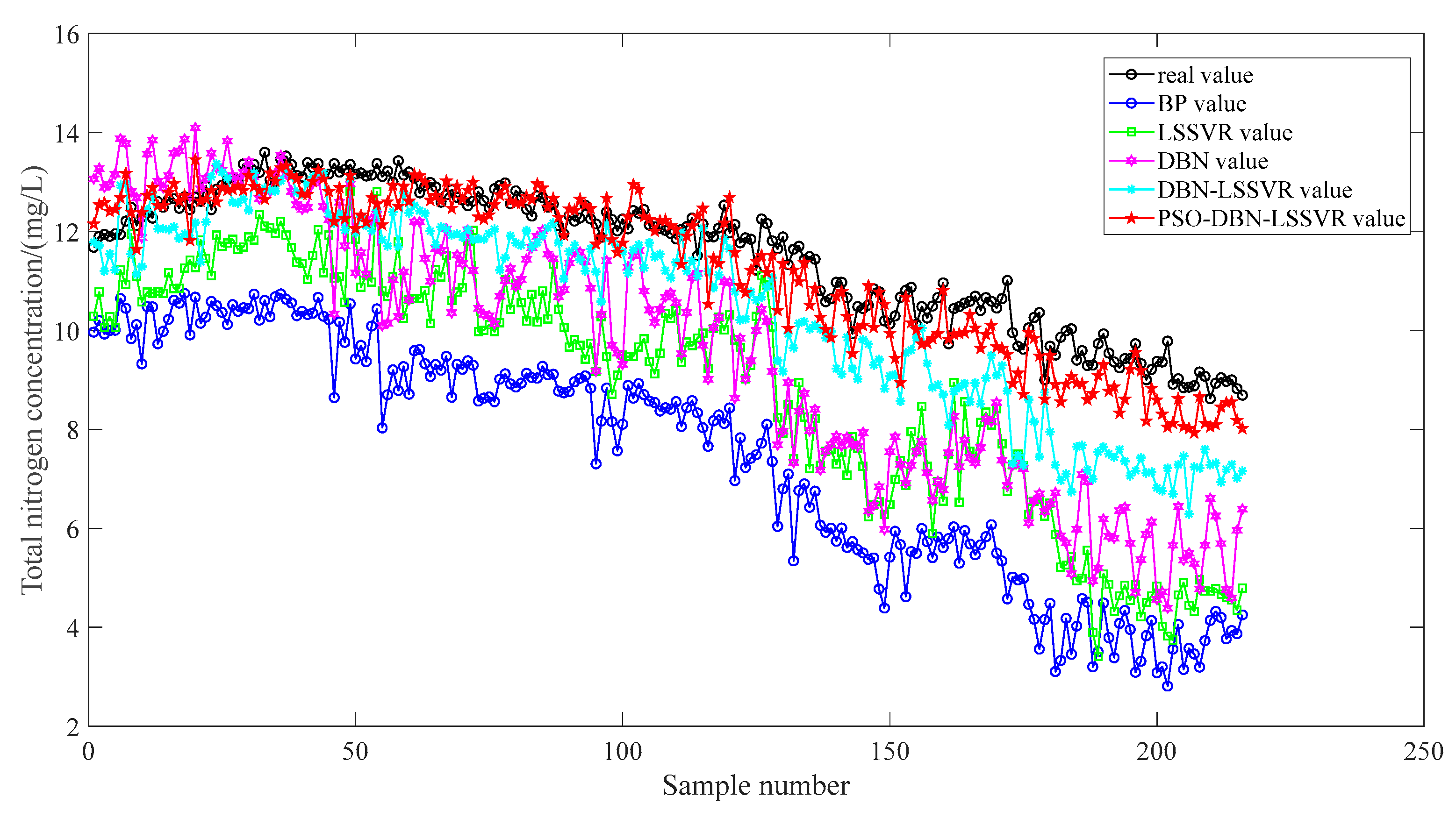
The prediction results are shown in Figure 6. It can be seen intuitively that the PSO-DBN-LSSVR prediction model proposed in this paper can be closer to the true value and has better prediction accuracy.

Figure 6. Model prediction results by the BP, LSSVR, DBN, DBN-LSSVR, and PSO-DBN-LSSVR.

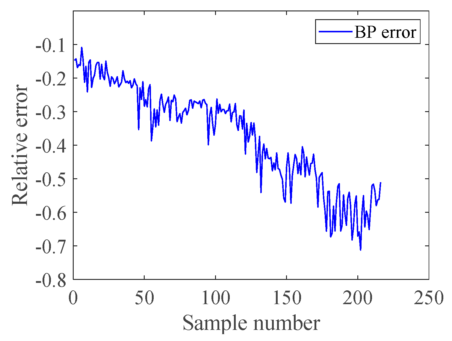
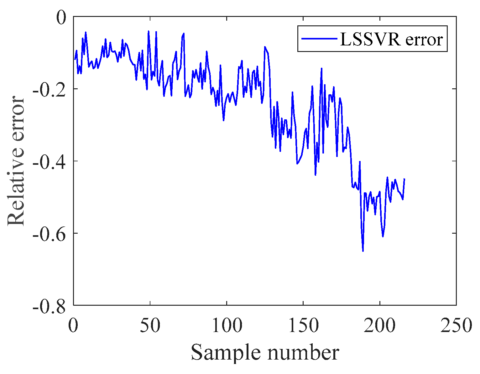
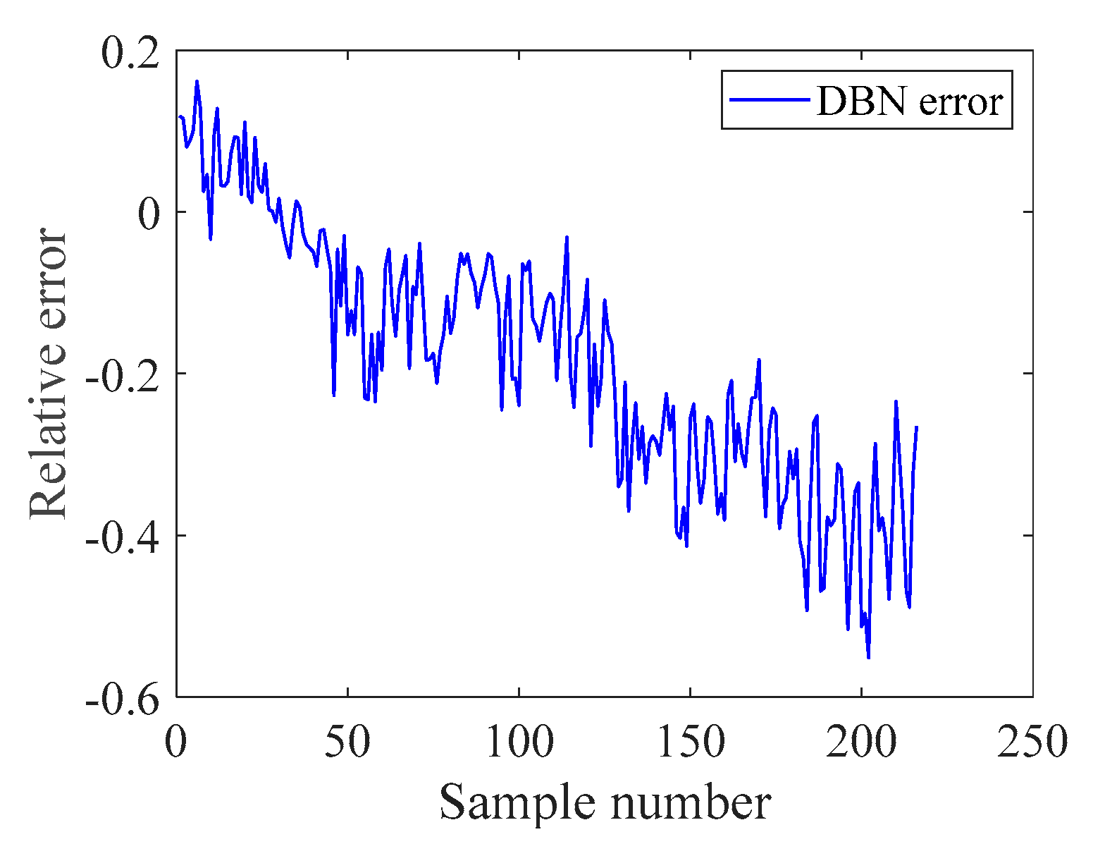
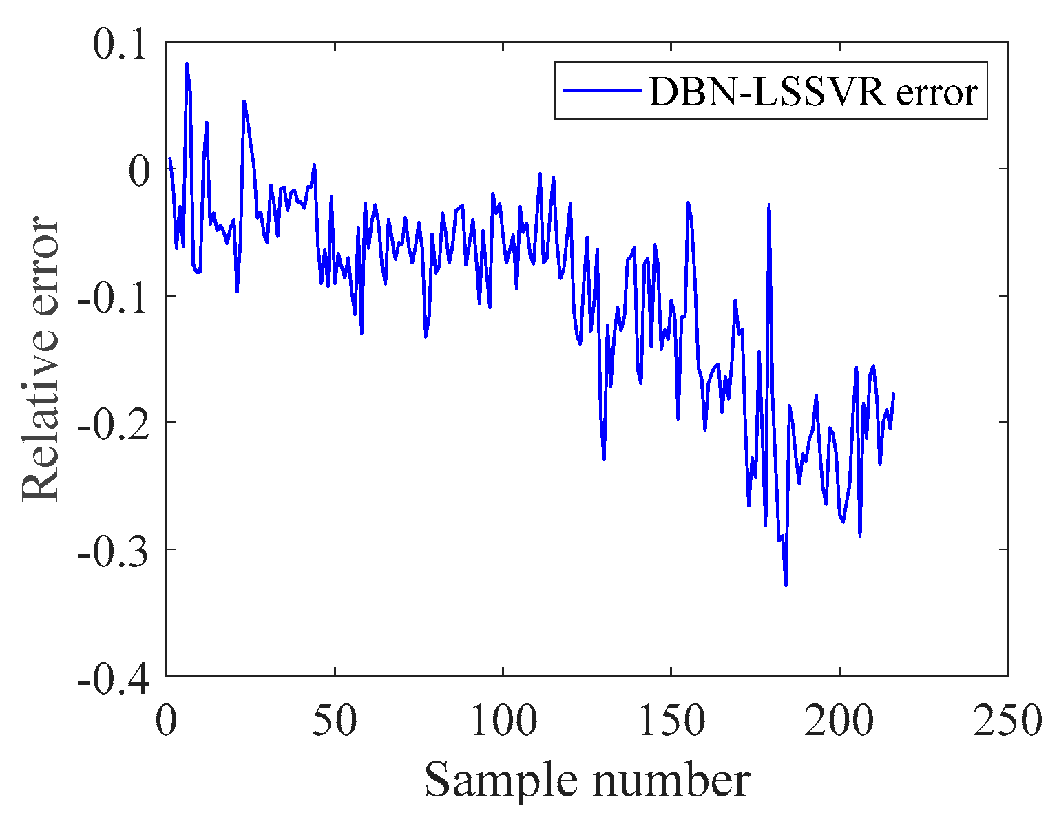
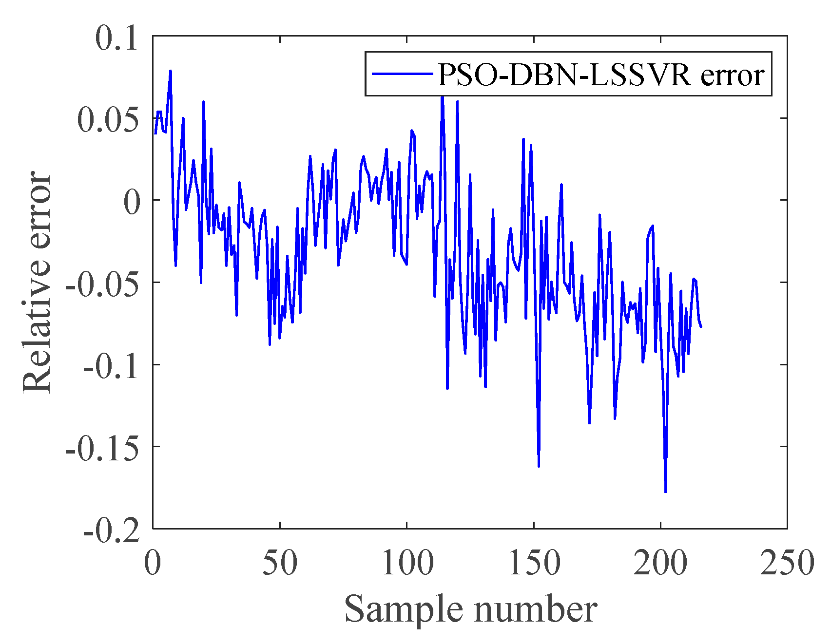
Figure 7, Figure 8, Figure 9, Figure 10 and Figure 11 show the prediction relative error curves of the models, which can be seen that the relative errors of the prediction results of the BP network, LSSVR, and DBN network are relatively large, and the error range was −0.8~0.2. Most of the results of the combined model DBN-LSSVR were maintained at −0.2~0.1, and a small part of the prediction results had large errors. The PSO-DBN-LSSVR model proposed in this paper had a relatively small prediction error, which was closer to 0, basically fluctuating around 0, and had better prediction accuracy.

Figure 7. BP network prediction relative error.

Figure 8. LSSVR prediction relative error.

Figure 9. DBN network prediction relative error.

Figure 10. DBN-LSSVR prediction relative error.

Figure 11. PSO-DBN-LSSVR model prediction relative error.

Table 1 demonstrates some of the predicted values of the total nitrogen content predicted by each model, that is, the comparison between the actual results and the true values in the next seven days.

Table 1. Comparison of model prediction results.

Time	Original Value (mg/L)	BP Value (mg/L)	LSSVR Value (mg/L)	DBN Value (mg/L)	DBN-LSSVR Value (mg/L)	PSO-DBN-LSSVR Value (mg/L)
2019-02-20 00:00	13.22	8.6979	10.6828	10.1474	11.7031	12.5979
2019-02-20 04:00	13	9.1988	11.0839	11.0232	12.3903	12.9361
2019-02-20 08:00	13.43	8.7839	11.7840	10.2788	11.6919	12.5109
2019-02-20 12:00	13.14	9.2670	10.2441	11.1805	12.7838	12.9132
2019-02-20 16:00	13.2	8.7083	10.6196	10.6156	12.3741	12.6128
2019-02-20 20:00	13.08	9.5872	10.6417	12.1926	12.5264	13.1486
2019-02-21 00:00	12.78	9.6111	10.6462	12.1894	12.4182	13.1224
2019-02-21 04:00	12.92	9.3237	10.8038	11.4544	12.3650	12.9969
2019-02-21 08:00	12.99	9.0675	10.1418	10.9945	12.0069	12.6309
2019-02-21 12:00	12.9	9.3087	11.2319	11.6579	11.7297	12.7271
2019-02-21 16:00	12.59	9.1945	11.0802	11.6121	12.0948	12.6160
2019-02-21 20:00	12.74	9.4751	11.5087	12.0508	12.0435	13.0189
2019-02-22 00:00	12.84	8.6493	10.6011	10.3545	11.924	12.4661
2019-02-22 04:00	12.69	9.3122	10.7719	11.5210	11.9509	12.9189
2019-02-22 08:00	12.64	9.2152	10.8572	11.3491	11.8826	12.6472
2019-02-22 12:00	12.52	9.3832	11.8051	12.0268	12.0394	12.8339
2019-02-22 16:00	12.61	9.2937	12.0186	11.2113	11.8317	12.9972
2019-02-22 20:00	12.8	8.5731	9.9736	10.4456	11.8490	12.2926
2019-02-23 00:00	12.62	8.6272	9.9999	10.3224	11.8396	12.2493
2019-02-23 04:00	12.48	8.6526	10.1130	10.2941	11.9544	12.3347
2019-02-23 08:00	12.86	8.5593	9.9745	10.1306	12.0480	12.5404
2019-02-23 12:00	12.93	9.0141	10.1563	10.6933	11.2165	12.7351
2019-02-23 16:00	12.98	9.1184	11.0300	11.0070	11.4718	12.9092
2019-02-23 20:00	12.56	8.9183	10.4243	11.2505	11.9139	12.6163
2019-02-24 00:00	12.82	8.8536	10.9359	10.8929	11.7686	12.5671
2019-02-24 04:00	12.7	8.9303	10.5588	11.0289	11.7201	12.5730
2019-02-24 08:00	12.45	9.1310	10.1881	11.4343	12.0153	12.7089
2019-02-24 12:00	12.31	9.0471	10.7265	11.6779	11.6864	12.6388
2019-02-24 16:00	12.72	9.0342	10.1683	11.8963	11.7758	12.9611
2019-02-24 20:00	12.68	9.2703	10.7973	12.0175	11.9109	12.8765
2019-02-25 00:00	12.49	9.1006	10.2320	11.5420	12.0775	12.4876
2019-02-25 04:00	12.55	9.1129	11.3385	11.4486	12.1674	12.6664
2019-02-25 08:00	12.12	8.7699	10.4254	10.6797	11.7704	12.2886
2019-02-25 12:00	11.95	8.7389	10.0619	10.8228	11.0445	11.9256
2019-02-25 16:00	12.32	8.7616	9.6618	11.3603	11.5961	12.4552
2019-02-25 20:00	12.21	8.9600	9.8102	11.5786	11.7213	12.4258
2019-02-26 00:00	12.27	9.0319	9.6956	11.5797	11.4317	12.6510
2019-02-26 04:00	12.53	9.0776	9.4178	11.3904	11.1997	12.5317
2019-02-26 08:00	12.25	8.8293	9.7401	10.8543	11.6494	12.4592
2019-02-26 12:00	12.15	7.3018	9.1662	9.1761	11.1869	11.7418
2019-02-26 16:00	11.88	8.1665	10.2781	10.3215	10.5819	11.8875
2019-02-26 20:00	12.39	8.8330	9.4702	11.4059	12.1509	12.6760

As can be seen from the model performance indicators in Table 2, compared with the single model BP, LSSVR, DBN, and the combined model DBN-LSSVR, performance indicators of PSO-DBN-LSSVR have been improved to varying degrees. MAE dropped from 4.0943, 2.8406, 2.6679, and 1.1290 to 0.4765. MAPE dropped from 36.99%, 19.86%, 24.54%, and 10.48% to 4.32%. RMSE dropped from 4.2746, 2.4957, 2.9354, and 1.3306 to 0.4877. And $R^2$increased from 0.2871, 0.6142, 0.6454, and 0.8714 to 0.9327, which achieved a relatively high fitting effect. From the performance index of the model, the model PSO-DBN-LSSVR established in this paper has achieved the relatively best results. Compared with the traditional BP model, MAE has dropped by 3.6178, MAPE has dropped by 32.67%, and RMSE has dropped by 3.7869, especially, $R^2$ increased by 0.6456. Compared with the single DBN model, MAE decreased by 2.1914, MAPE decreased by 20.22%, RMSE decreased by 2.4477, and $R^2$increased by 0.2873. In terms of running time, the average training time of BP, LSSVR, and DBN are 12, 420, and 128 s, respectively. Although the combined model takes a long time, the best prediction accuracy is obtained to meet the requirements of engineering applications. It can be demonstrated from the analysis that the PSO-DBN-LSSVR prediction model we developed is superior to the shallow BP and LSSVR models, as well as the DBN and DBN-LSSVR models, which can better predict the total nitrogen content of the water quality of the cross-section in the next four hours. As can be seen from the determination coefficient, the prediction model also has better accuracy and robustness.

Table 2. Comparison of the model performance index.

Model	MAE	MAPE (%)	RMSE	${\mathit{R}}^2$
BP	4.0943	36.99	4.2746	0.2871
LSSVR	2.8406	19.86	2.4957	0.6142
DBN	2.6679	24.54	2.9354	0.6454
DBN-LSSVR	1.1290	10.48	1.3306	0.8714
PSO-DBN-LSSVR	0.4765	4.32	0.4877	0.9327

4. Conclusions

In order to solve the problem that the traditional prediction method is difficult to fully excavate the essential characteristics of the water quality of the cross-section, resulting in low prediction accuracy of the water quality parameters, in this paper, we proposed a deep learning method based on DBN to predict the water quality of the cross-section. Used deep belief network to learn and extract water quality features based on historical water quality data at a given time, and then combined LSSVR to predict value changes of water quality in the future. To overcome the shortcoming that the random initialization of the DBN network parameter will affect model prediction performance, the particle swarm optimization algorithm is used to optimize the model weight parameters to enhance the model prediction performance. At the top layer of the model, LSSVR is applied to predict water quality parameters. The experimental results indicated that the PSO-DBN-LSSVR cross-section water quality prediction model constructed in this paper can organically integrate feature extraction and non-linear regression methods, which greatly reduced the error between the prediction result and the actual value, and effectively improved the prediction accuracy of water quality parameters. Specifically, it provides technical support for the precise control of the water quality of the cross-section and also has a certain role in the management of water pollution.

In order to make the water quality prediction model more practical, in future research, we will collect more water quality data such as heavy metal parameters, flow, etc., and increase the input feature parameters of the neural network. Also, optimize the existing deep belief network structure further to improve the accuracy of the prediction model.

References

1. Cabral Pinto, M.M.S.; Ordens, C.M.; de Melo, M.T.C.; Inácio, M.; Almeida, A.; Pinto, E.; da Silva, E.A.F. An inter-disciplinary approach to evaluate human health risks due to long-term exposure to contaminated groundwater near a chemical complex. Exp. Health 2020, 12, 199–214. [Google Scholar] [CrossRef]
2. Cabral-Pinto, M.M.S.; Marinho-Reis, A.P.; Almeida, A.; Ordens, C.M.; Silva, M.M.; Freitas, S.; da Silva, E.A.F. Human predisposition to cognitive impairment and its relation with environmental exposure to potentially toxic elements. Environ. Geochem. Health 2018, 40, 1767–1784. [Google Scholar] [CrossRef]
3. Nguyen, H.D.; Che, D.L.; Pham, V.T. Application of a Neural Network Technique for Prediction of the Water Quality Index in the Dong Nai River, Vietnam. J. Environ. Sci. Eng. B 2016, 7, 363–370. [Google Scholar]
4. Lai, Y.C.; Yang, C.P.; Hsieh, C.Y.; Wu, C.Y.; Kao, C.M. Evaluation of non-point source pollution and river water quality using a multimedia two-model system. J. Hyd. 2011, 409, 583–595. [Google Scholar] [CrossRef]
5. Huang, J.; Liu, N.; Wang, M.; Yan, K. Application WASP model on validation of reservoir-drinking water source protection areas delineation. In Proceedings of the 2010 3rd International Conference on Biomedical Engineering and Informatics, Yantai, China, 16–18 October 2010; pp. 3031–3035. [Google Scholar]
6. Warren, I.; Bach, H. MIKE21: A modeling system for estuaries, coastal waters and seas. Environ. Soft. 1992, 7, 229–240. [Google Scholar] [CrossRef]
7. Hayes, D.F.; Labadie, J.W.; Sanders, T.G. Enhancing water quality in hydropower system operations. Water Resour. Res. 1998, 34, 471–483. [Google Scholar] [CrossRef]
8. Tang, G.; Li, J.; Zhu, Z.; Li, Z.; Nerry, F. Two-dimensional water environment numerical simulation research based on EFDC in Mudan River, Northeast China. In Proceedings of the 2015 IEEE European Modelling Symposium (EMS), Madrid, Spain, 6–8 October 2015; pp. 238–243. [Google Scholar]
9. Aly, A.H.; Peralta, R.C. Optimal Design of Aquifer Cleanup Systems under Uncertainty Using a Neural Network and a Genetic Algorithm. Water Resour. Res. 1999, 35, 2523–2532. [Google Scholar] [CrossRef]
10. Tirabassi, M.A. A statistically based mathematical water quality model for a non-estuarine river system. J. Am. Water Resour. Assoc. 1971, 7, 1221–1237. [Google Scholar] [CrossRef]
11. Hu, L.; Zhang, C.; Hu, C.; Jiang, G. Use of grey system for assessment of drinking water quality: A case S study of Jiaozuo city, China. In Proceedings of the IEEE International Conference on Grey Systems and Intelligent Services, Nanjing, China, 10–12 November 2009; pp. 803–808. [Google Scholar]
12. Batur, E.; Maktav, D. Assessment of surface water quality by using satellite images fusion based on PCA method in the Lake Gala, Turkey. IEEE Trans. Geosci. Rem. Sens. 2019, 57, 2983–2989. [Google Scholar] [CrossRef]
13. Jaloree, S.; Rajput, A.; Sanjeev, G. Decision tree approach to build a model for water quality. Bin. J. Data Min. Net. 2014, 4, 25–28. [Google Scholar]
14. Liu, J.T.; Yu, C.; Hu, Z.H.; Zhao, Y.C. Accurate prediction scheme of water quality in smart mariculture with deep Bi-S-SRU learning network. IEEE Access 2020, 8, 24784–24798. [Google Scholar] [CrossRef]
15. Khan, K.; See, C.S. Predicting and analyzing water quality using machine learning: A comprehensive model. In Proceedings of the IEEE Long Island Systems Applications and Technology Conference (LISAT), Farmingdale, NY, USA, 29–29 April 2016; pp. 1–6. [Google Scholar]
16. Liao, H.; Sun, W. Forecasting and evaluating water quality of Chao Lake based on an improved decision tree method. Proc. Environ. Sci. 2010, 2, 970–979. [Google Scholar] [CrossRef]
17. Li, X.; Song, J. A new ANN-Markov chain methodology for water quality prediction. In Proceedings of the International Joint Conference on Neural Networks, Killarney, Ireland, 12–17 July 2015; pp. 1–6. [Google Scholar]
18. Ahmed, A.M.; Shah, S.M.A. Application of adaptive neuro-fuzzy inference system (ANFIS) to estimate the biochemical oxygen demand (BOD) of Surma River. J. King. Saud. Univ. Eng. Sci. 2015, 12, 237–243. [Google Scholar] [CrossRef]
19. Yan, J.Z.; Xu, Z.B.; Yu, Y.C.; Xu, H.X.; Gao, K.L. Application of a hybrid optimized BP network model to estimate water quality parameters of Beihai Lake in Beijing. Appl. Sci. 2019, 9, 1863. [Google Scholar] [CrossRef]
20. Yan, L.; Qian, M. AP-LSSVM modeling for water quality prediction. In Proceedings of the 31st Chinese Control Conference, Hefei, China, 25–27 July 2012; pp. 6928–6932. [Google Scholar]
21. Solanki, A.; Aggarwal, H.; Khare, K. Predictive analysis of water quality parameters using deep learning. Int. J. Comput. Appl. 2015, 125, 975–8887. [Google Scholar] [CrossRef]
22. Ghesu, F.C. Marginal space deep learning: Efficient architecture for volumetric image parsing. IEEE Trans. Med. Imag. Vol. 2016, 35, 1217–1228. [Google Scholar] [CrossRef]
23. Tu, Y.; Du, J.; Lee, C. Speech enhancement based on teacher–student deep learning using improved speech presence probability for noise-robust speech recognition. IEEE/ACM Trans. Audio Speech Lang Process. 2019, 27, 2080–2091. [Google Scholar] [CrossRef]
24. Lee, K.P.; Wu, B.H.; Peng, S.L. Deep-learning-based fault detection and diagnosis of air-handling units. Build. Environ. 2019, 157, 24–33. [Google Scholar] [CrossRef]
25. Sun, C.; Ma, M.; Zhao, Z.; Tian, S.; Yan, R.; Chen, X. Deep transfer learning based on sparse autoencoder for remaining useful life prediction of tool in manufacturing. IEEE Trans. Ind. Inf. 2019, 15, 2416–2425. [Google Scholar] [CrossRef]
26. Mughees, A.; Tao, L. Multiple deep-belief-network-based spectral-spatial classification of hyperspectral images. Tsinghua Sci. Technol. 2019, 24, 183–194. [Google Scholar] [CrossRef]
27. Karimi, M.; Majidi, M.; MirSaeedi, H.; Arefi, M.M.; Oskuoee, M. A novel application of deep belief networks in learning partial discharge patterns for classifying corona, surface, and internal discharges. IEEE Trans. Ind. Electron. 2020, 67, 3277–3287. [Google Scholar] [CrossRef]
28. Huang, W.; Song, G.; Hong, H.; Xie, K. Deep architecture for traffic flow prediction: Deep belief networks with multitask learning. IEEE Trans. Intell. Trans. Syst. 2014, 15, 2191–2210. [Google Scholar] [CrossRef]
29. Zhu, K.; Xun, P.; Li, W.; Li, Z.; Zhou, R. Prediction of passenger flow in urban rail transit based on big data analysis and deep learning. IEEE Access 2019, 7, 142272–142279. [Google Scholar] [CrossRef]
30. Cheng, Y.; Zhou, X.; Wan, S.; Choo, K.R. Deep belief network for meteorological time series prediction in the Internet of things. IEEE Int. Things J. 2019, 6, 4369–4376. [Google Scholar] [CrossRef]
31. Marir, N.; Wang, H.; Feng, G.; Li, B.; Jia, M. Distributed abnormal behavior detection approach based on deep belief network and ensemble SVM using spark. IEEE Access 2018, 6, 59657–59671. [Google Scholar] [CrossRef]
32. Fadlullah, Z.M.; Tang, F.; Mao, B.; Liu, J.; Kato, N. On intelligent traffic control for large-scale heterogeneous networks: A value matrix-based deep learning approach. IEEE Commun. Lett. 2018, 22, 2479–2482. [Google Scholar] [CrossRef]
33. Bengio, Y. Learning deep architectures for AI. Found. Trends Mach. Learn. 2009, 2, 1–127. [Google Scholar] [CrossRef]
34. Nicolas, L.R.; Yoshua, B. Representational power of restricted boltzmann machines and deep belief networks. Neural Comput. 2008, 20, 1631–1649. [Google Scholar]
35. Hinton, G.E. Training products of experts by minimizing contrastive divergence. Neural Comput. 2002, 14, 1771–1800. [Google Scholar] [CrossRef]
36. Kennedy, J.; Eberhart, R. Particle swarm optimization. In Proceedings of the IEEE International Conference on Neural Networks, Perth, Australia, 27 November–1 December 1995; pp. 1942–1948. [Google Scholar]
37. Xu, L.Q.; Liu, S.Y. Water quality prediction model based on APSO-WLSSVR. Eng. Sci. 2014, 42, 80–86. [Google Scholar]
Article Metrics
Citations
Article Access Statistics
Multiple requests from the same IP address are counted as one view.