Effect of Open Boundary Conditions and Bottom Roughness on Tidal Modeling around the West Coast of Korea

Abstract

The aim of this study was to investigate the effect of open boundary conditions and bottom roughness on the tidal elevations around the West Coast of Korea (WCK) using an open-source computational fluids dynamics tool, the TELEMAC model. To obtain a detailed tidal forcing at open boundaries, three well-known assimilated tidal models—the Finite Element Solution (FES2014), the Oregon State University TOPEX/Poseidon Global Inverse Solution Tidal Model (TPXO9.1) and the National Astronomical Observatory of Japan (NAO.99Jb)—have been applied to interpolate the offshore tidal boundary conditions. A number of numerical simulations have been performed for different offshore open boundary conditions, as well as for various uniform and non-uniform bottom roughness coefficients. The numerical results were calibrated against observations to determine the best fit roughness values for different sub-regions within WCK. In order to find out the dependence of the tidal elevation around the WCK on the variations of open boundary forcing, a sensitivity analysis of coastal tide elevation was carried out. Consequently, it showed that the tidal elevation around the WCK was strongly affected by local characteristics, rather than by the offshore open boundary conditions. Eventually, the numerical results can provide better quantitative and qualitative tidal information around the WCK than the data obtained from assimilated tidal models.

1. Introduction

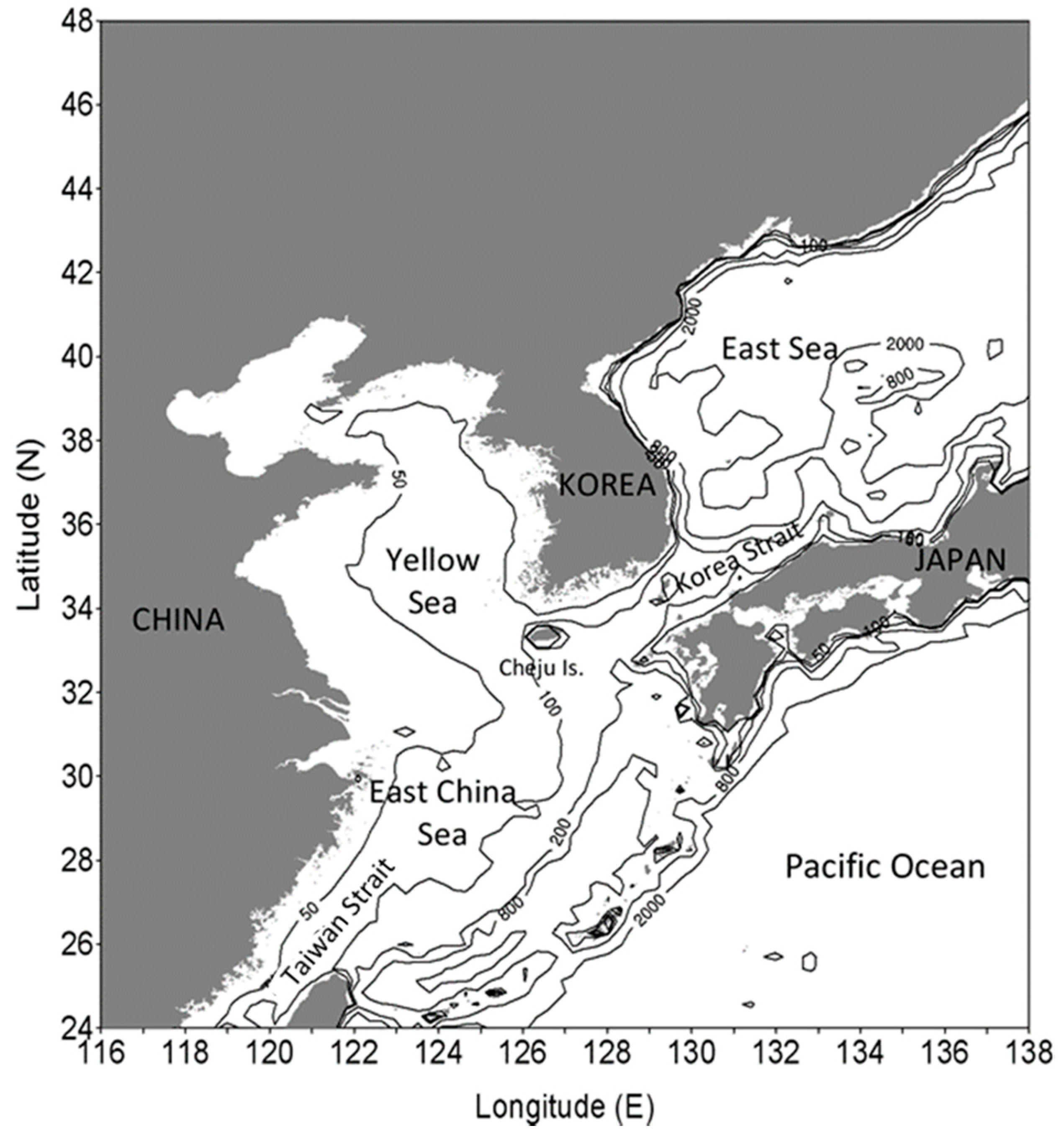
The Yellow Sea (YS) is located between the mainland of China and the Korean Peninsula, and its depth is about 44 m on average, with a maximum depth of 152 m. The sea bottom slope gradually rises toward the East China coast and more abruptly toward the Korean Peninsula, and the depth gradually increases from north to south. Southern YS is bounded by the East China Sea (ECS) along a line running northeastward from the mouth of the Changjiang River to the southwestern tip of Korea. ECS covers the area originating around the Taiwan Strait at about 25° N, extending northeastward to the Kyushu Island, Japan, and to the Korea Strait, and bounded by the Ryukyu Island chains on the southeastern open ocean (Figure 1). On the broad and shallow shelf under the Yellow and the East China Sea (YECS), the flow is dominated by strong semidiurnal M2 tidal currents with the superimposition of semidiurnal S2, diurnal K1 and O1 currents [1,2,3,4]. Approaching the WCK, the tidal amplitudes vary from 4 to 8 m, and the speed of the tidal current may increase to more than 1.56 m/s near the coasts.

Along with strong tidal currents, the WCK is surrounded by lots of islands including extremely irregular and indented coastlines, the tidal propagation and shoaling processes on the shore in this broad flat region are very complicated and sensitive to the variation of tidal elevation.

The study on the tidal circulation in this region has been carried out by various authors, such as Le Fevre et al. [5], Kim [6], Naimie et al. [7], and Suh [8] using 2D depth-averaged finite element models on unstructured grids, or Choi [2], Tang [9], Kantha et al. [10], Kang et al. [11] and Lee et al. [12] using 3-D finite difference models on structured grids. However, there are still very few authors using data obtained from different assimilated tidal models to set up the offshore boundary conditions. Most authors have applied a constant boundary forcing condition (BFC) or tidal charts, such as Ogura’s chart [1,2,13,14]) and Nishida’s chart [3,15,16] or applied a very coarse observation data combined with partly constant boundary forcing conditions [11,17]. Only Le Fevre et al. [5] and Suh [8] have applied tidal charts from FES 94.1 and FES 2004 models for OBC. Using FVCOM, we recently applied a tidal chart from NAO.99Jb. In principle, the tidal information around the WCK can be obtained from assimilated global and regional tidal models [18].

In principle, the tidal information around the WCK can be obtained from assimilated global and regional tidal models. The assimilation model, which is a combination of a dynamical model and observed data, was actively advanced in the research group of the modern global tide model, and pioneered by [19]. By the assimilation model, the problem of the empirical method with regard to the resolution can be compensated by a hydrodynamic model, and any inadequate potential of the hydrodynamic model can be recovered by observed data [20]. Recently, using the unprecedented sea surface height data of satellite altimeter TOPEX/POSEIDON (T/P), several research groups have developed highly accurate assimilation models especially in an open ocean ([5,20,21,22,23,24]). T/P was launched on 10 August 1992, which measures sea level relative to the ellipsoid with an overall accuracy of approximately 5 cm [25]. Due to the high accuracy of T/P altimeter data for those assimilation models, it can be used to extract relatively accurate tidal boundary conditions around the marginal sea within YECS.

Among the global assimilation models, FES2014 (https://www.aviso.altimetry.fr/en/data/products/auxiliary-products/global-tide-fes.html) and TPXO9.1 (http://volkov.oce.orst.edu/tides/tpxo9_atlas.html) atlases are open to the public and can be freely downloaded. The FES2014 atlas was produced by Legos and CLS Space Oceanography Division, and distributed by Aviso, with support from CNES (https://datastore.cls.fr/catalogues/fes2014-tide-model/). It is distributed as a tidal chart on grid resolution of 1/16° based on the dynamical finite element tide model CEFMO, and data assimilation code CADOR. The finite element grid of the model CEFMO has about 2,900,000 computational nodes and covered 34 tidal constituents. In addition to above two global tide models, the regional tide model NAO.99Jb (https://www.miz.nao.ac.jp/staffs/nao99/index_En.html) was developed by Matsumoto et al. (2000) for the region around Japan with a resolution of 1/12°, covering from 110 to 165° E and from 20–65° N so that YECS was entirely included in this region. This model was nested with the global model NAO.99b to provide open boundary conditions to the regional model and the assimilation was performed with both T/P data and 219 coastal tidal gauges obtained around Japan and Korea. Most T/P-derived altimetric tides can be inaccurate in shallow coastal oceans because the resolution enforced on data analysis by the spatial resolution of T/P is simply inadequate near ocean margins.

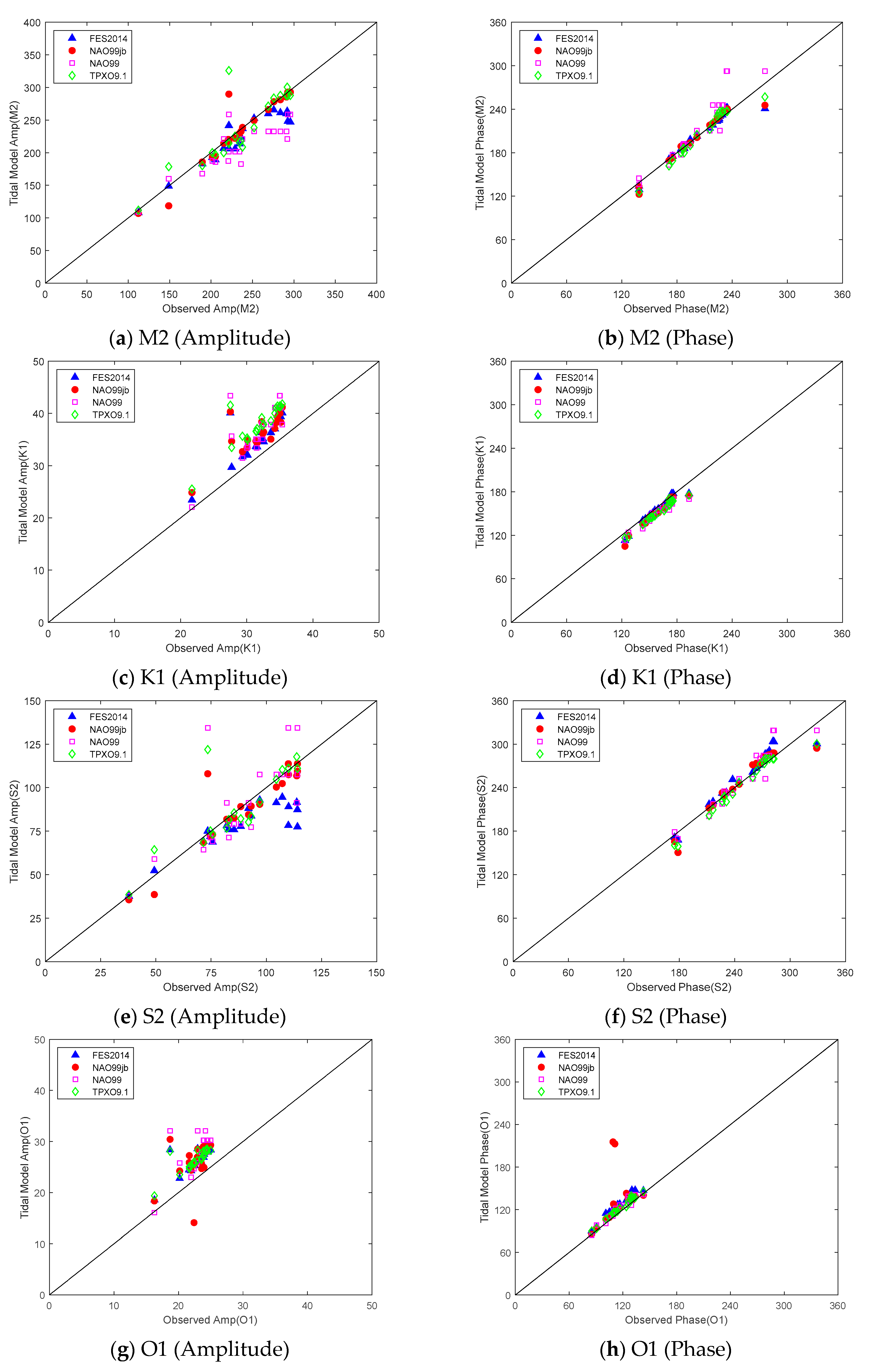
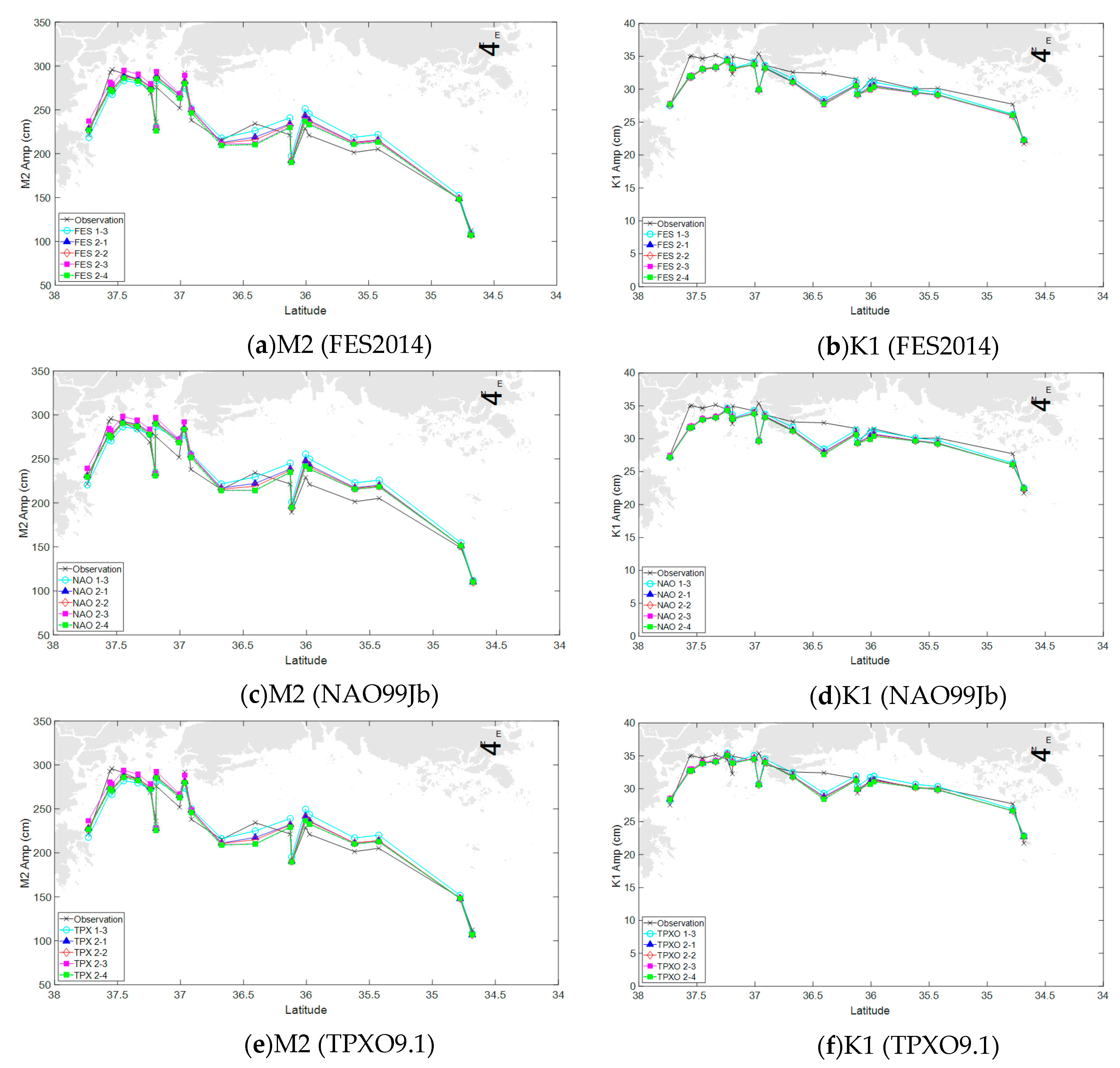
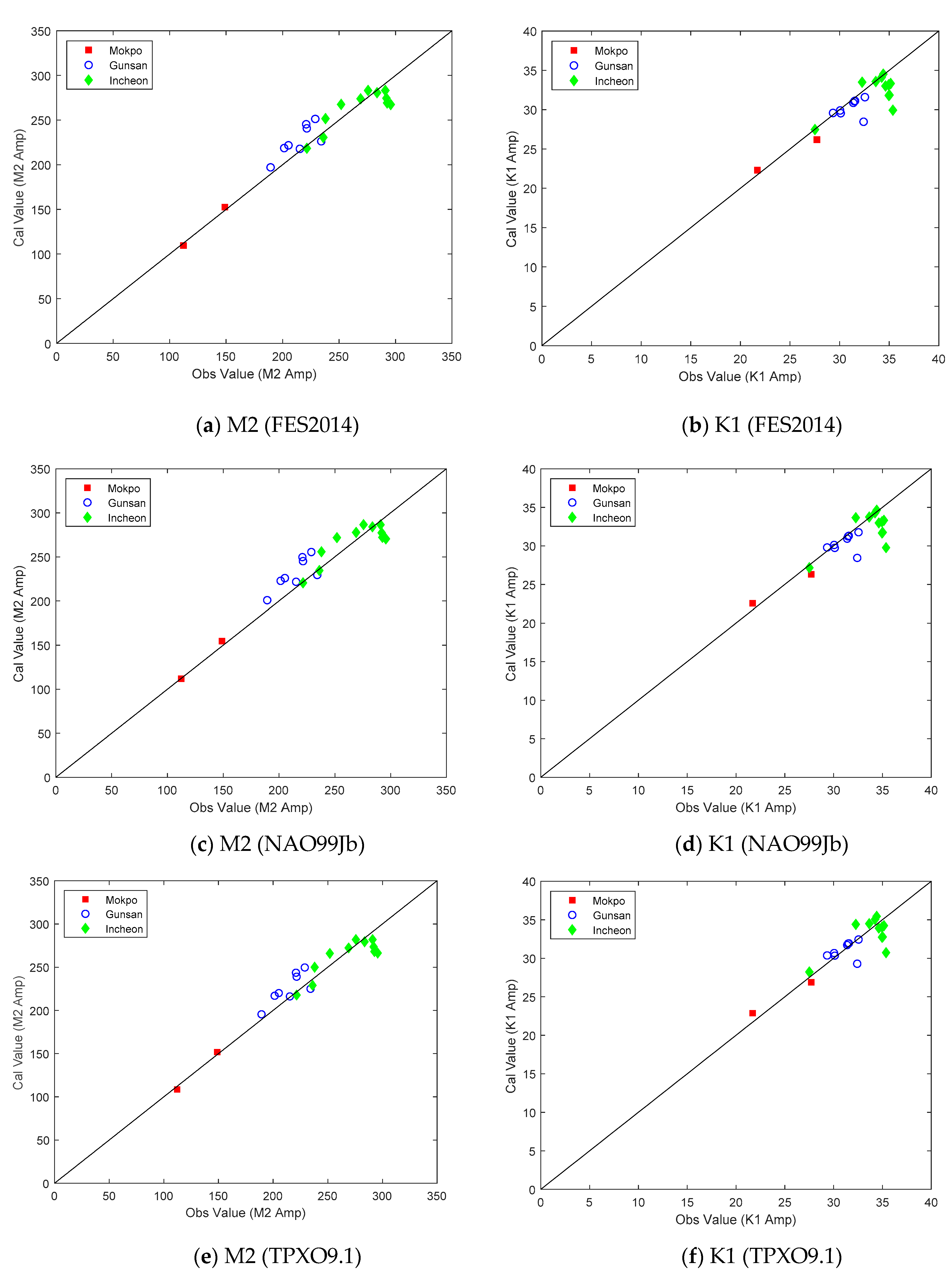
Therefore, we first validated the tidal information of tidal constituents $K_1, O_1, M_2 \mathrm{and} S_2$ provided by three assimilated tidal models; FES2014, NAO99Jb and TPXO9.1 against the observation at 21 tidal gauges along WCK. Figure 2 shows the comparison of amplitude (left) and phase (right) obtained from the assimilated tidal models with observation data obtained from gauging stations along the WCK. It shows that while the phases are better agreement with observation, the amplitudes obtained from the assimilated tidal models still poorly agreed with the observed data. More detailed quantitative comparisons between the amplitude and phase obtained from the assimilated tidal models and observation data are shown in

Table A1. Validation of amplitude and phase obtained from three tidal models against observation data.

Tidal Constituent		RMSE			Range of Amplitudes and Phases
		FES2014 (1/16°)	NAO99Jb (1/12°)	TPXO9.1 (1/6°)
M2	Amp (cm)	20.2	16.1	25	107.3 $÷$ 295.8
	Phase (°)	8.2	5.4	6.6	36.8 $÷$ 275.6
K1	Amp (cm)	4.2	4.9	6.2	21.7 $÷$ 35.4
	Phase (°)	5.4	7.6	7.5	75.6 $÷$ 193.1
S2	Amp (cm)	14.6	8.4	11.4	37.8 $÷$ 114.1
	Phase (°)	10.9	8.8	7.1	59.6 $÷$ 328.9
O1	Amp (cm)	3.8	4.8	3.9	16.3 $÷$ 25
	Phase (°)	11	31.8	6.1	39 $÷$ 142.9

(in Appendix A). Wherein it shows NAO99Jb provides a better agreement of the amplitude for the constituents $M_2 \mathrm{and} S_2$, while FES2014 provides a little better fit of the amplitude for $K_1 \mathrm{and} O_1$. It also shows the constituent M2 has the largest amplitude in comparison with other tidal constituents; about 5–8 times, 2.5–2.8 times, and 6.6–11.8 times larger than K1, S2 and O1 amplitudes, respectively.

In addition, the resolutions (1/6°, 1/12° and 1/16°) of three tidal models are not fine enough along the coastlines, so they cannot provide enough detailed quantitative and qualitative tidal information along the WCK. Therefore, in order to obtain more detail on tidal information along the WCK, an accuracy numerical simulation with higher grid resolutions is needed.

This study is to introduce several numerical investigations using higher grid resolutions and applying different open boundary conditions extracted from three well-known assimilated tidal models FES2014, TPXO9.1 and NAO.99Jb then calibrated with different uniform and non-uniform bottom roughness values for different sub-regions within WCK to investigate the effect of open boundary condition and bottom roughness on the tidal elevations from major constituents (M2, K1, S2 and O1) around the West Coast of Korea.

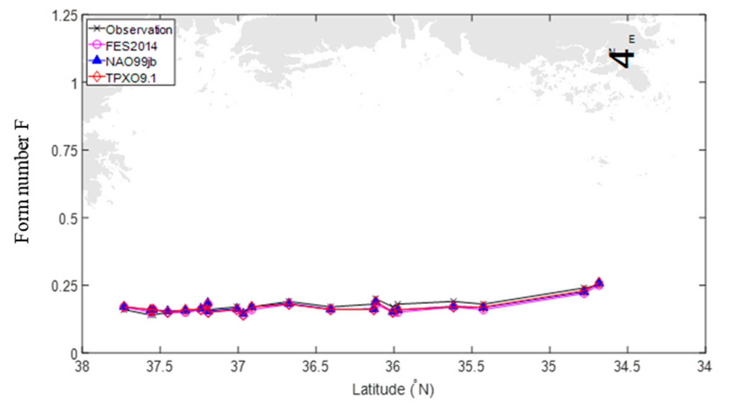
Based on the form number (F), the ratio of the amplitudes of $K_1, O_1, M_2, and S_2$ suggested by [26] is shown in Equation (1).

$$F=\frac{K_1+O_1}{M_2+S_2}$$

(1)

whereby the mixed tide is classified following the value of the form number F; if the value of F less than 0.25 or larger than 1.25, then it is classified as semidiurnal or diurnal, respectively. Otherwise, if the value of F is located between 0.25 and 1.25, it is considered mixed.

Figure 3 shows the values of the form number along the WCK are below 0.25 according to the data obtained from observation at 21 tidal gauges, as well as from three assimilated tidal models, FES2014, TPXO9.1 and NAO.99Jb; therefore, the mixed tide prevails semidiurnal in the WCK.

2. Numerical Modeling

As mentioned above, since the study region was quite shallow, the numerical simulation was based on an open-source software, the TELEMAC-2D (http://www.opentelemac.org) model. It is well-known software with an abundant history of development and application over many years in fluvial and maritime hydraulics [27,28]. The TELEMAC-2D is capable of capturing the complicated bathymetry and coastlines of the WCK surrounded by lots of islands including extremely irregular and indented coastlines by using unstructured grids.

2.1. Basic Equations

The TELEMAC-2D has solved the depth-averaged Navier-Stokes equations with two-equation turbulence closure models (k-ε) using the finite element method, as follows:

The continuity equation

$$\frac{\partial h}{\partial t}+\frac{\partial \left(hU\right)}{\partial x}+\frac{\partial \left(hV\right)}{\partial y}=0$$

(2)

and momentum equations

$$\frac{\partial \left(hU\right)}{\partial t}+\frac{\partial \left(hUU\right)}{\partial x}+\frac{\partial \left(hUV\right)}{\partial y}=-h·g\frac{\partial Z}{\partial x}+h·F_x+\mathrm{div}\left(h·{\nu }_e·\overrightarrow{\nabla }\left(U\right)\right)$$

(3)

$$\frac{\partial \left(hV\right)}{\partial t}+\frac{\partial \left(hUV\right)}{\partial x}+\frac{\partial \left(hVV\right)}{\partial y}=-h·g\frac{\partial Z}{\partial y}+h·F_y+\mathrm{div}\left(h·{\nu }_e·\overrightarrow{\nabla }\left(V\right)\right)$$

(4)

$$\frac{\partial k}{\partial t}+U\frac{\partial k}{\partial x}+V\frac{\partial k}{\partial y}=\frac{1}{h} \mathrm{div}\left(h·\frac{{\nu }_t}{{\sigma }_k} \overrightarrow{\nabla }\left(k\right)\right)+P-\epsilon +P_{kv}$$

(5)

$$\frac{\partial \epsilon }{\partial t}+U\frac{\partial \epsilon }{\partial x}+V\frac{\partial \epsilon }{\partial y}=\frac{1}{h} \mathrm{div}\left(h·\frac{{\nu }_t}{{\sigma }_k} \overrightarrow{\nabla }\left(\epsilon \right)\right)+\frac{\epsilon }{k}\left(c_{1\epsilon }P-c_{2\epsilon }\epsilon \right)+P_{\epsilon v}$$

(6)

where h is the water depth; U and V are the depth averaged velocity components;

$U=\frac{1}{h}{{\displaystyle \int }}_{Z_f}^{Z}udz$ and $V=\frac{1}{h}{{\displaystyle \int }}_{Z_f}^{Z}vdz$

Z and Z_f are the free surface and bottom elevations, respectively;

F_x and F_y are body forces in x and y directions including Coriolis ($F_x^c,F_y^c)$, bottom friction $F_x^f,F_y^f)$, and surface wind $F_x^w,F_y^w)$ forces determined as $F_x=F_x^c+F_x^f+F_x^w$ and $F_y=F_y^c+F_y^f+F_y^w$

Coriolis force; $F_x^c=2\omega \sin \left(\lambda \right)v$ and $F_y^c=-2\omega \sin \left(\lambda \right)u$; $\omega =7.292 \times {10}^{-5}$ is angular and $\lambda$ is latitude;

Bottom friction force; $F_x^f=-\frac{1}{2h}{C}_{f}U\sqrt{U^2+V^2}$ and $F_y^f=-\frac{1}{2h}{C}_{f}V\sqrt{U^2+V^2}$, where C_f is the bottom friction coefficient, $C_f=\frac{g{n}^2}{h^{1/3}}$, n is Manning’s coefficient;

Wind forcing on the free surface is neglected; i.e., ($F_x^w,F_y^w$) = 0.

And ${\nu }_e$ is the effective viscosity, the summation of the molecular viscosity ν and the turbulent viscosity ν_t ${\nu }_e=\nu +{\nu }_t$; where

$${\nu }_t=c_{\mu }\frac{k^2}{\epsilon }.$$

(7)

The depth averaged kinetic energy k and its dissipation rate ε are:

$$k=\frac{1}{h}{{\displaystyle \int }}_{Z_f}^Z\frac{1}{2}\overline{u_i^{\prime }{u}_i^{\prime }}dz \mathsf{and} \epsilon =\frac{1}{h}{{\displaystyle \int }}_{Z_f}^Z\nu \overline{\frac{\partial u_i^{\prime }}{\partial x_j}\frac{\partial u_i^{\prime }}{\partial x_j}}dz$$

where $u_i^{\prime }$ is the fluctuating velocity and the overbar represents an average over time; i.e., $u_i=U_i+u_i^{\prime }$; U_i (=U or V) is an average over time of velocity components; and P is the production term:

$$P={\nu }_t\left(\frac{\partial U_i}{\partial x_j}+\frac{\partial U_j}{\partial x_i}\right)\frac{\partial U_i}{\partial x_j}$$

(8)

P_kv and P_εv are vertical shear terms: $P_{kv}=c_k\frac{u_{*}^3}{h}; P_{\epsilon v}=c_{\epsilon }\frac{u_{*}^4}{h^2}$ where $c_k=\frac{1}{\sqrt{c_f}}$ and $c_{\epsilon }=3.6\frac{c_{2\epsilon }\sqrt{c_{\mu }}}{c_f{}^{3/4}}$

$u_{*}$ is the friction velocity: $u_{*}=\sqrt{\frac{C_f}{2}\left(U^2+V^2\right)}$

The empirical constants in Equations (5) and (6) $C_{\mu }=0.09, C_{1\epsilon }=1.44, C_{2\epsilon }=1.92, {\sigma }_k=1.0 and {\sigma }_{\epsilon }=1.3$ of the k-ε model are obtained from classical test cases.

2.2. Boundary Conditions

2.2.1. At the Solid Boundary

On the solid boundary, such as coastline and bottom, the no-slip condition is applied; i.e., velocity $\overrightarrow{U}=\left(U, V\right)=\left(0, 0\right)$.

In this region, particularly near the shallow coastline, the effect of bottom friction becomes prominent, the bottom friction is calculated by:

$${\tau }_b=\left({\tau }_{bx}, {\tau }_{by}\right)=-\frac{1}{2}\rho C_f\sqrt{U^2+V^2}\left(U, V\right)$$

(9)

The value of the coefficient C_f is obtained from the calibration procedure, which is shown in Section 3.1 below.

The boundary condition for turbulence kinetic energy and its dissipation are defined as

$$k_{\delta }=\frac{u_{*}^2}{\sqrt{C_{\mu }}}+\frac{C_{2\epsilon }}{C_{\epsilon }{C}_f}{u}_{*}^2 \mathsf{and} {\epsilon }_{\delta }=\frac{u_{*}^3}{\kappa \delta }+\frac{1}{\sqrt{C_f}}\frac{u_{*}^3}{h}$$

(10)

where δ is a distance from the wall, $\delta =0.1$ of a local mesh size; $u_{*}$ is friction velocity of the wall.

2.2.2. At the Free Surface

We assume the wind force on the free surface is neglected as mentioned above, i.e., $F_x^w=F_y^w=0$.

2.2.3. At the Open Boundary

Tidal harmonic parameters obtained from each assimilated tidal models FES2014, NAO99Jb and TPXO9.1 were combined into the open boundary conditions, as follows: $H={\displaystyle \sum }_i{H}_i$

$$H_i\left(M, t\right)=A_{F_i}\left(M\right)\cos \left(2\pi \frac{t}{T}-{\phi }_{F_i}\left(M\right)\right)$$

(11)

where H_i is the water elevation, $A_{F_i}$ is amplitude; T is period and ${\phi }_{F_i}$ is phase of each tidal constituent.

In this study, four major tidal constituents M2, K1, S2 and O1, were considered. The harmonic constants of tidal constituents for open boundary conditions were obtained from three assimilated tidal models; FES2014, TPXO9.1 and NAO.99Jb.

Turbulence kinetic energy and its dissipation at the open boundary were set as:

$k=C_{2\epsilon }\frac{P_{kv}^2}{P_{\epsilon v}}$ and $\epsilon =P_{kv}$.

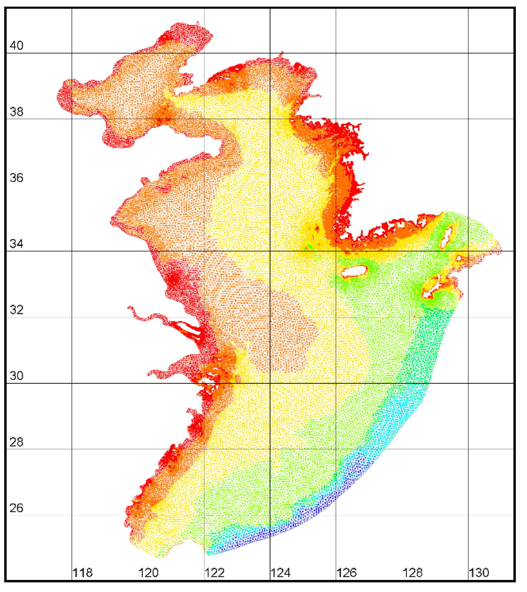
2.3. Study Region

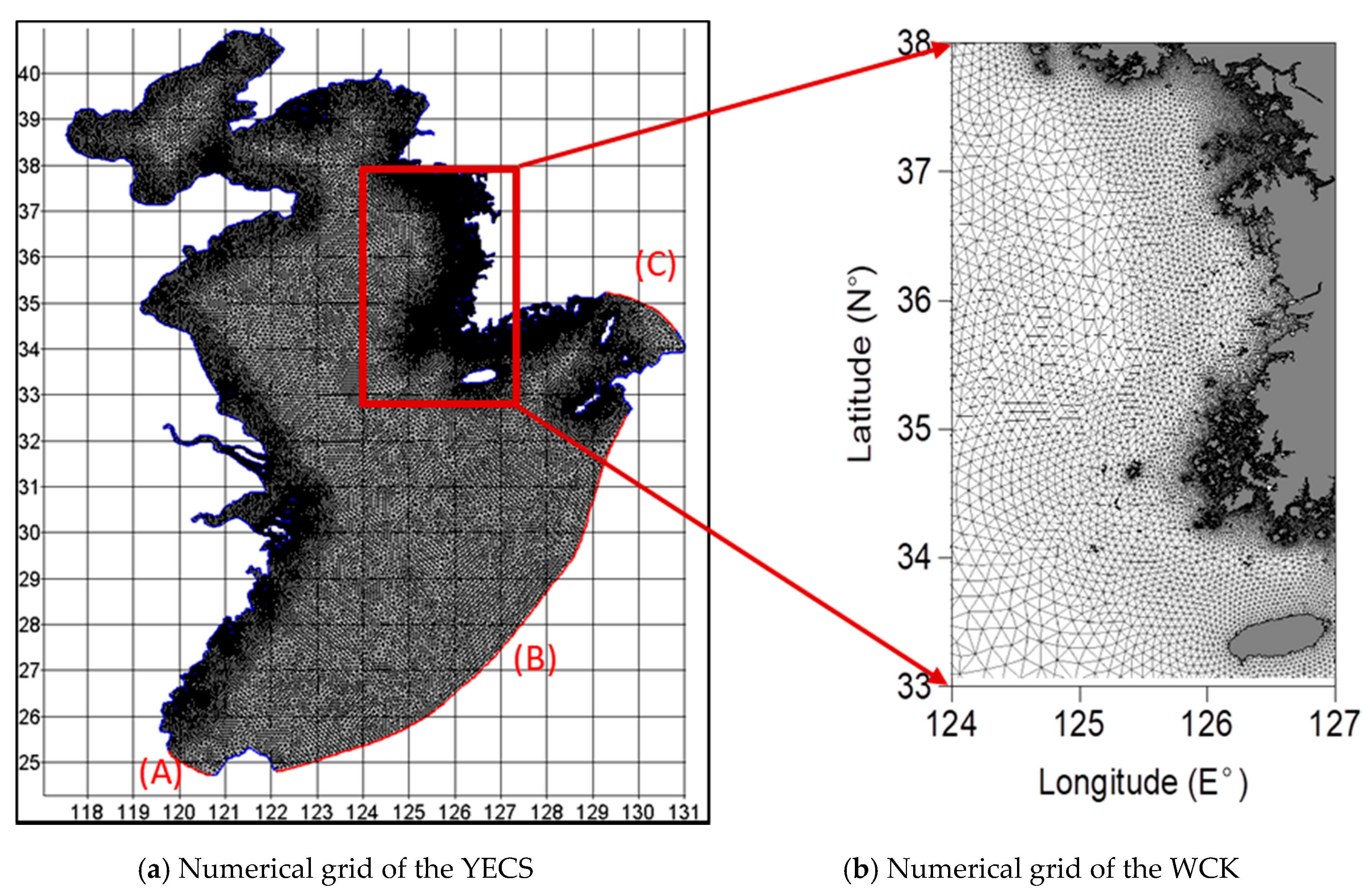
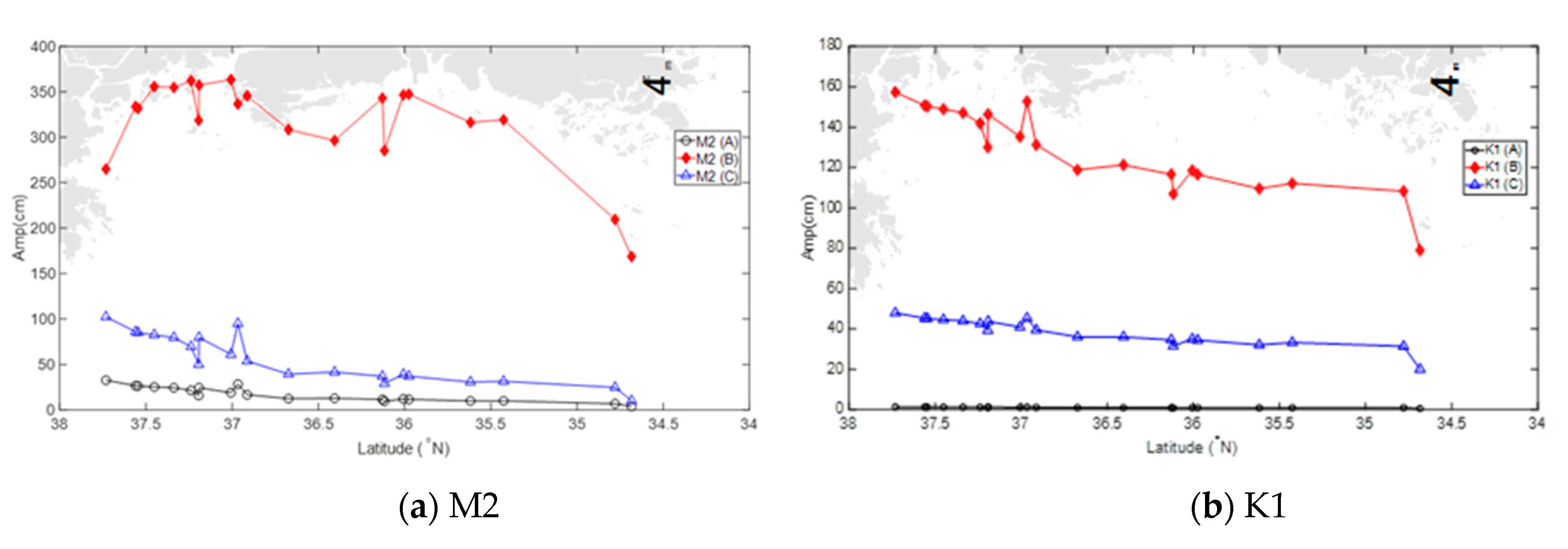
The study area covered the entire YS and most of the ECS in spherical coordinate. The bathymetry data of 30 arc-seconds resolution was downloaded from the General Bathymetric Chart of the Ocean (GEBCO2014: https://www.ngdc.noaa.gov/mgg/ibcm/ibcmdvc.html) as shown in Figure 4. The shorelines with an accuracy of about 250 m were downloaded from the NOAA shoreline website (https://shoreline.noaa.gov). This region included the flat and broad continental shelf of YECS, bounded by Taiwan Strait (A), a line of shelf-break determined by 200 m isobaths (B), and Korea Strait (C), as shown in Figure 5. The open boundary was expanded to the shelf edge of YECS which was advantageous to use offshore co-oscillating tidal conditions as a boundary forcing in order to minimize disturbances by the geographical configuration and nonlinear tidal response near-shore. Open boundaries adjacent to the offshore also enabled the numerical results around WCK to minimize the influence of unexpected numerical instabilities at open boundaries.

In this study, the numerical simulation applied a hybrid horizontal resolution of an unstructured grid using a free pre-processing Blue Kenue software tool (https://nrc.canada.ca/en/research-development/products-services/software-applications/blue-kenuetm-software-tool-hydraulic-modellers). Herein the unstructured triangular grid had a horizontal resolution varying from 0.2 to 1 km in the WCK, 3–5 km in the East coast of China, and 9–12 km in the interior of YS and ECS. After running a number of simulations to check for grid independence, the final grid of 203,927 grid cells was used for the simulation in this study. Bathymetry was interpolated to each nodal point of the horizontal grid using Blue Kenue software as well (Figure 5).

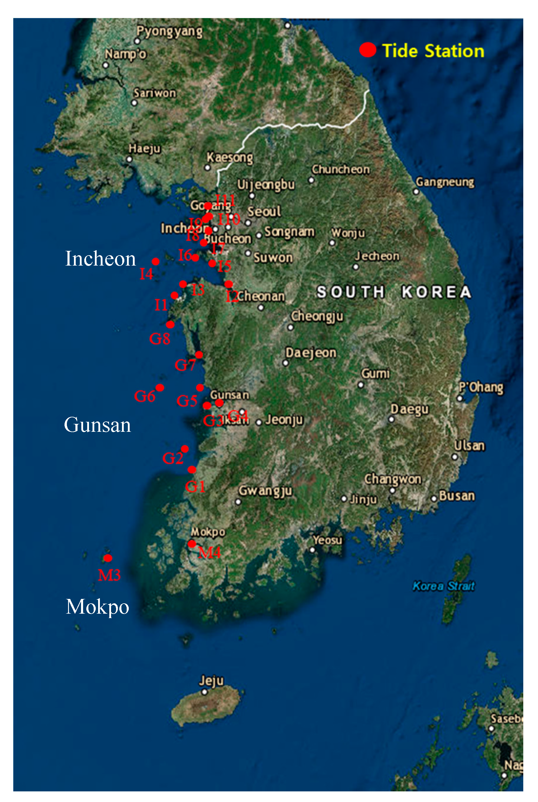
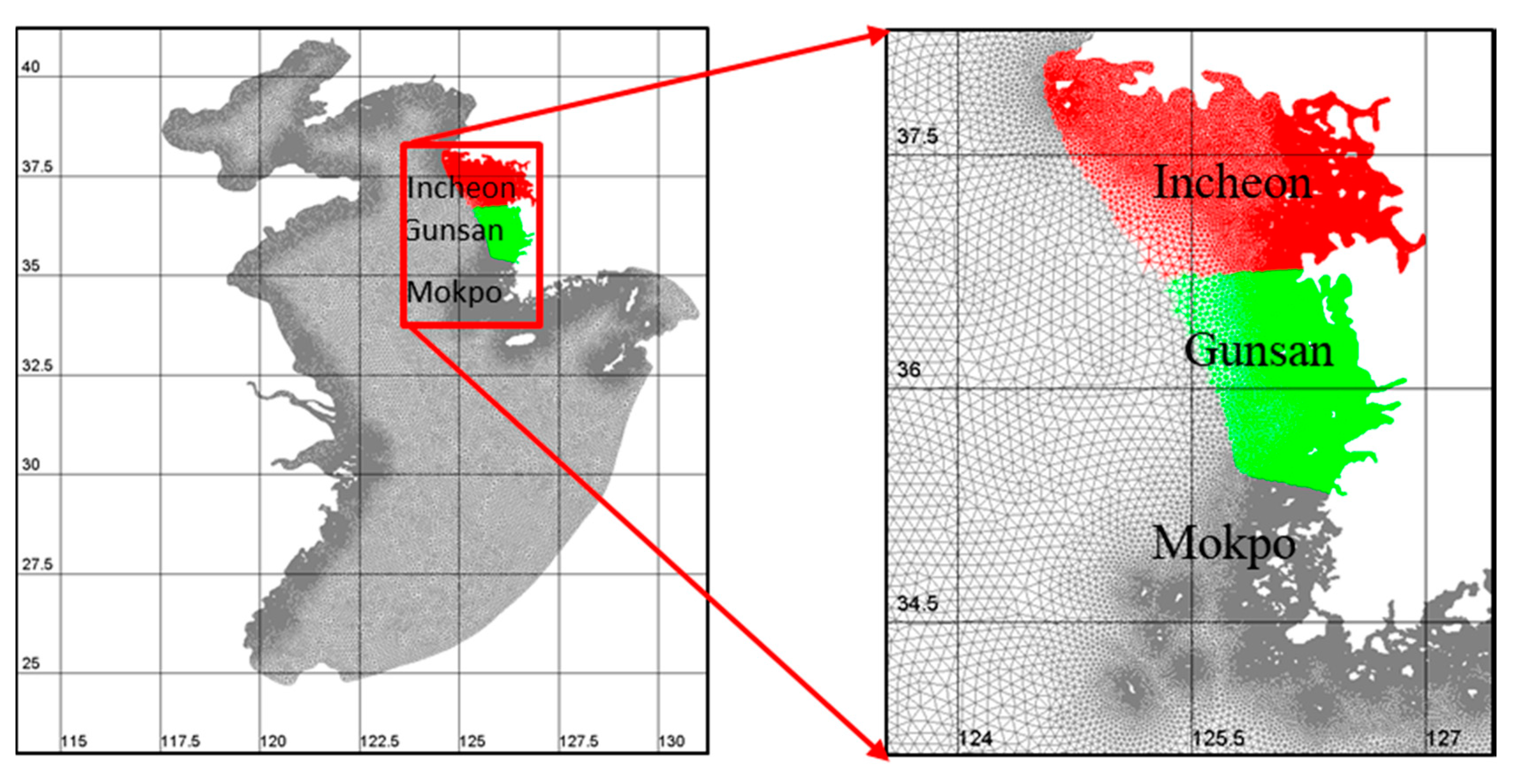
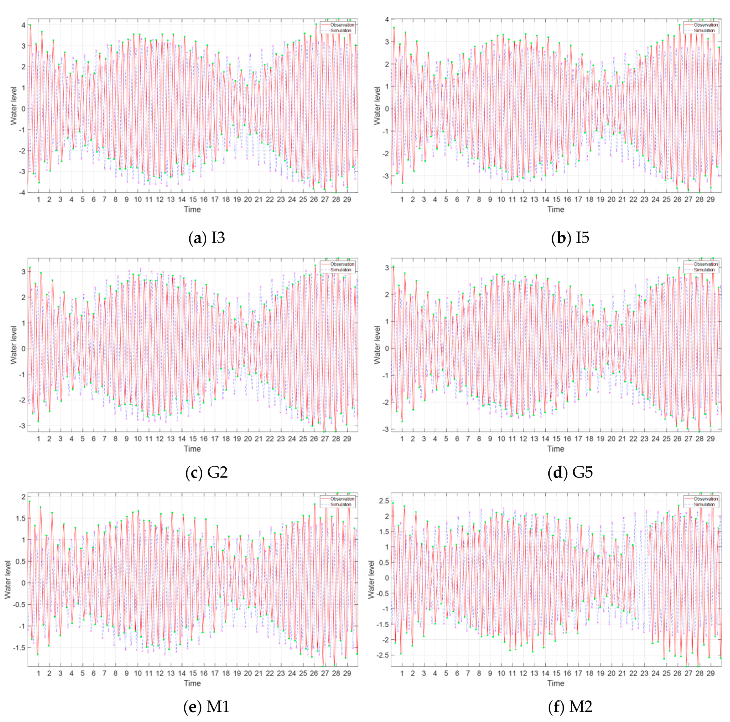
A total of 21 tidal gauges were collected around the WCK to provide the observed tidal elevation data of semidiurnal M2 and S2 and diurnal K1 and O1 constituents in YECS. As shown in Figure 6, the WCK can be divided into three sub-regions based on the common characteristics of their bathymetry and coastlines—the first region was Kyunggi Bay near Incheon (I), the second region was around the estuary of the Geum River near Gunsan (G), and the third region was around the south-western tip near Mokpo (M). The numbers of tidal gauges located in three regions Mokpo, Gunsan and Incheon were 2, 8 and 11, respectively. The most recent observation data in 2017 downloaded from Korea Hydrographic and Oceanographic Agency (http://www.khoa.go.kr/koofs/kor/observation/obs_real.do) have been selected for the calibration and validation of numerical models.

3. Numerical Results and Discussion

The numerical simulations were carried out on our high-performance computing cluster (http://cfdlabsnu.com) for the real-time simulation of 60 days with time step of 20 s. The numerical results obtained from the last 30 days simulation were used for the following analyses.

3.1. Response of the Tide around WCK to the Bottom Roughness

3.1.1. Applying Uniform Roughness Coefficient

Previous tidal calculations in the YECS region were mostly using the quadratic bottom friction law, in which the typical value of roughness coefficient $C_f$ was chosen as a uniform value of 0.0025, as shown in [2,16,29,30]. We again have verified the numerical model with various uniform roughness coefficients that ranged from 0.0015 to 0.03 for different offshore open boundary conditions (OBCs) interpolated from three assimilated tidal models (FES2014, TPXO9.1 and NAO.99Jb).

The WCK was divided into three different sub-regions—Mokpo (M), Gunsan (G), and Incheon (I)—as shown in Figure 7, for applying different bottom friction coefficients. The borderline of this sub-regions was set based on a water depth contour of around 50 m. Different values of bottom friction coefficient were applied with regards to the geographic characteristics.

As shown in

Table A2. RMSE results obtained from uniform roughness bottom for FES2014.

Tidal Model	Constituent	Cd	RMSE (cm)
			Mokpo (M)	Gunsan (G)	Incheon (I)	Mean
FES2014	M2	0.0015	10.17	34.83	40.18	36.30
		0.002	5.67	22.87	16.62	18.63
		0.0023	3.22	16.49	14.39	14.59
		0.0025	2.79	12.99	19.28	16.12
		0.003	6.24	10.58	35.57	26.63
	K1	0.0015	0.79	1.46	2.07	1.77
		0.002	0.98	1.30	2.03	1.70
		0.0023	1.16	1.48	2.34	1.96
		0.0025	1.29	1.70	2.64	2.21
		0.003	1.67	2.35	3.51	2.97
	S2	0.0015	2.63	10.94	12.21	11.15
		0.002	1.29	6.92	19.21	14.55
		0.0023	1.58	6.24	23.41	17.38
		0.0025	2.16	6.59	26.12	19.35
		0.003	3.76	8.99	31.90	23.77
	O1	0.0015	1.42	1.71	1.33	1.49
		0.002	1.82	2.38	1.86	2.07
		0.0023	1.99	2.67	2.26	2.40
		0.0025	2.10	2.86	2.53	2.63
		0.003	2.43	3.38	3.27	3.24

,

Table A3. RMSE results obtained from uniform roughness bottom for NAO99Jb.

Tidal Model	Constituent	Cd	RMSE (cm)
			Mokpo (M)	Gunsan (G)	Incheon (I)	Mean
NAO99Jb	M2	0.0015	12.90	40.56	45.18	41.37
		0.002	7.38	26.96	19.39	21.89
		0.0023	4.14	19.93	14.16	16.06
		0.0025	2.29	15.75	17.64	16.07
		0.003	4.40	10.46	33.32	25.00
	K1	0.0015	0.95	1.65	2.17	1.90
		0.002	1.04	1.35	2.13	1.78
		0.0023	1.17	1.47	2.42	2.01
		0.0025	1.28	1.64	2.70	2.24
		0.003	1.64	2.30	3.60	3.01
	S2	0.0015	2.62	11.03	12.85	11.56
		0.002	1.53	7.07	19.89	15.05
		0.0023	1.82	6.39	24.02	17.84
		0.0025	2.37	6.77	26.70	19.78
		0.003	4.03	9.32	32.58	24.31
	O1	0.0015	0.49	0.84	1.49	1.21
		0.002	0.83	1.21	1.22	1.19
		0.0023	1.05	1.53	1.46	1.46
		0.0025	1.19	1.75	1.69	1.67
		0.003	1.54	2.28	2.37	2.27

and

Table A4. RMSE results obtained from uniform roughness bottom for TPXO9.1.

Tidal Model	Constituent	Cd	RMSE (cm)
			Mokpo (M)	Gunsan (G)	Incheon (I)	Mean
TPXO9.1	M2	0.0015	10.49	34.68	40.07	36.19
		0.002	5.33	21.39	15.72	17.51
		0.0023	3.29	15.14	14.63	14.16
		0.0025	3.25	12.13	19.90	16.26
		0.003	7.42	11.13	36.85	27.64
	K1	0.0015	1.12	2.02	2.46	2.20
		0.002	0.99	1.36	1.91	1.65
		0.0023	1.01	1.21	1.93	1.62
		0.0025	1.06	1.25	2.10	1.74
		0.003	1.31	1.75	2.87	2.37
	S2	0.0015	2.17	10.22	12.63	11.13
		0.002	1.05	6.53	19.79	14.88
		0.0023	1.70	6.26	24.07	17.85
		0.0025	2.26	6.76	26.51	19.65
		0.003	4.07	9.54	32.34	24.17
	O1	0.0015	1.07	1.31	1.24	1.25
		0.002	1.46	1.95	1.55	1.71
		0.0023	1.70	2.33	1.98	2.10
		0.0025	1.80	2.50	2.25	2.31
		0.003	2.18	3.09	3.00	2.97

(in Appendix A), based on the evaluation of root mean square deviation (RMSE) of tidal amplitudes between the observation and the numerical results obtained from applying various uniform roughness coefficients, the results show that the numerical results were very distinct from each other. For the tidal constituent M2, the bottom roughness coefficient C_f = 0.0023 provides the best result obtained from FES2014 and TPXO9.1, while the numerical results obtained from NAO99Jb were not significantly different between C_f = 0.0023 and 0.0025. For the tidal constituent K1, the bottom roughness coefficient C_f = 0.002 provides the best result obtained from NAO99Jb, while the numerical results obtained from FES2014 were not significantly different between C_f = 0.0015 and 0.002; the numerical results obtained from TPXO9.1 were not significantly different between C_f = 0.002, 0.0023 and 0.0025. For the tidal constituent S2, the bottom roughness coefficient C_f = 0.0015 provides the best result obtained from all three assimilated tidal models. For the tidal constituent O1, the bottom roughness coefficient C_f = 0.0015 provides the best result obtained from FES2014 and TPXO9.1, while the numerical results obtained from NAO99Jb were not significantly different between C_f = 0.0015 and 0.002. In addition, based on the RMSE values in Table A2, Table A3 and Table A4, the results show that for M2 the most appropriate roughness values for Mokpo, Gunsan and Incheon regions were 0.0025, 0.003 and 0.0023, respectively. Whereas, for S2, the most appropriate roughness values for Mokpo, Gunsan and Incheon regions were 0.002, 0.0023 and 0.0015, respectively. For O1, the most appropriate roughness value for Mokpo, Gunsan and Incheon regions was 0.0015 and for K1 the most appropriate roughness values with FES2014 and NAO99Jb for Mokpo, Gunsan and Incheon regions were 0.0015, 0.002 and 0.002, respectively. However, with TPXO9.1 the values for Mokpo, Gunsan and Incheon regions were 0.002, 0.0023 and 0.002, respectively.

3.1.2. Applying Non-Uniform Roughness Coefficient

As shown above, applying a uniform bottom roughness coefficient for the entire WCK was inappropriate. According to the bathymetry data, the bottom slope was relatively milder in the Incheon region than in Mokpo and Gunsan regions. In addition, there were lots of islands around the Mokpo region rather than the Incheon region. We can expect that more energy dissipation occurred in the Mokpo and Gunsan regions than in the Incheon region. The larger values of the bottom friction coefficient were applied to Mokpo and Gunsan regions than the Incheon region. In addition, the roughness coefficient values for the Gunsan region were set to be the largest because its bed form was more variable than the Mokpo region.

Table A5. List of simulation cases applying non-uniform bottom roughness coefficients to different sub-regions of WCK.

Case	Tide Model	Bottom Friction Coefficient
		Mokpo	Gunsan	Incheon	Other Sub-Region
FES 2-1	FES2014	0.0025	0.0027	0.002	0.002
FES 2-2	FES2014	0.0025	0.003	0.002	0.002
FES 2-3	FES2014	0.0025	0.0035	0.0018	0.002
FES 2-4	FES2014	0.0025	0.0035	0.002	0.002
NAO 2-1	NAO99Jb	0.0025	0.0027	0.002	0.002
NAO 2-2	NAO99Jb	0.0025	0.003	0.002	0.002
NAO 2-3	NAO99Jb	0.0025	0.0035	0.0018	0.002
NAO 2-4	NAO99Jb	0.0025	0.0035	0.002	0.002
TPX 2-1	TPXO9.1	0.0025	0.0027	0.002	0.002
TPX 2-2	TPXO9.1	0.0025	0.003	0.002	0.002
TPX 2-3	TPXO9.1	0.0025	0.0035	0.0018	0.002
TPX 2-4	TPXO9.1	0.0025	0.0035	0.002	0.002

shows the list of simulation cases applying non-uniform bottom roughness coefficients to different sub-regions Mokpo, Gunsan, Incheon and other regions within WCK. As shown in

Table A6. RMSE results obtained from non-uniform roughness bottom for M2.

Tidal Constituent	Simulation Case	RMSE (cm)
		Mokpo	Gunsan	Incheon	Mean
M2	FES 2-1	3.33	12.04	11.94	11.44
	FES 2-2	3.26	11.77	11.90	11.31
	FES 2-3	3.29	11.61	12.12	11.37
	FES 2-4	3.65	11.40	12.06	11.27
	NAO 2-1	2.25	15.00	12.75	13.09
	NAO 2-2	2.25	14.15	12.38	12.53
	NAO 2-3	2.27	13.39	13.83	13.00
	NAO 2-4	2.26	13.53	12.03	12.09
	TPX 2-1	4.10	11.09	11.91	11.08
	TPX 2-2	3.74	11.17	11.91	11.10
	TPX 2-3	3.88	11.18	11.68	10.97
	TPX 2-4	3.79	11.24	12.09	11.23

,

Table A7. RMSE results obtained from non-uniform roughness bottom for K1.

Tidal Constituent	Simulation Case	RMSE (cm)
		Mokpo	Gunsan	Incheon	Mean
K1	FES 2-1	1.28	1.75	2.32	2.04
	FES 2-2	1.30	1.87	2.37	2.11
	FES 2-3	1.28	2.01	2.28	2.10
	FES 2-4	1.23	1.92	2.30	2.08
	NAO 2-1	1.28	1.72	2.42	2.09
	NAO 2-2	1.28	1.81	2.43	2.12
	NAO 2-3	1.28	1.96	2.36	2.13
	NAO 2-4	1.28	1.95	2.46	2.18
	TPX 2-1	1.04	1.32	1.90	1.63
	TPX 2-2	1.05	1.38	1.90	1.65
	TPX 2-3	1.05	1.50	1.84	1.66
	TPX 2-4	1.05	1.49	1.91	1.69

,

Table A8. RMSE results obtained from non-uniform roughness bottom for S2.

Tidal Constituent	Simulation Case	RMSE (cm)
		Mokpo	Gunsan	Incheon	Mean
S2	FES 2-1	2.25	6.92	22.09	16.56
	FES 2-2	2.13	7.25	22.04	16.58
	FES 2-3	2.14	8.08	20.63	15.75
	FES 2-4	1.94	7.81	21.98	16.63
	NAO 2-1	2.38	7.03	22.60	16.94
	NAO 2-2	2.39	7.52	22.91	17.23
	NAO 2-3	2.37	8.29	21.31	16.27
	NAO 2-4	2.37	8.31	23.28	17.62
	TPX 2-1	2.38	7.10	22.36	16.78
	TPX 2-2	2.34	7.61	22.72	17.12
	TPX 2-3	2.30	8.40	21.09	16.14
	TPX 2-4	2.31	8.43	23.03	17.48

and

Table A9. RMSE results obtained from non-uniform roughness bottom for O1.

Tidal Constituent	Simulation Case	RMSE (cm)
		Mokpo	Gunsan	Incheon	Mean
O1	FES 2-1	2.13	2.95	2.44	2.62
	FES 2-2	2.18	3.06	2.51	2.71
	FES 2-3	2.14	3.09	2.48	2.70
	FES 2-4	2.12	3.07	2.43	2.67
	NAO 2-1	1.21	1.82	1.62	1.67
	NAO 2-2	1.20	1.86	1.62	1.68
	NAO 2-3	1.22	1.97	1.62	1.73
	NAO 2-4	1.21	1.95	1.65	1.74
	TPX 2-1	1.91	2.70	2.22	2.39
	TPX 2-2	1.83	2.64	2.17	2.33
	TPX 2-3	1.82	2.71	2.16	2.36
	TPX 2-4	1.87	2.77	2.24	2.42

, once the non-uniform bottom roughness coefficients were applied, the mean RMSE values for M2 from the varied ranged of 14–36 cm down to a value of about 11 cm with OBCs obtained from FES2014 and TPXO9.1. These values varied from 16–41 cm down to 12–13 cm with OBCs obtained from NAO99Jb while, there was no significant improvement for K1, S2 and O1. In the WCK, M2 was the dominant constituent, followed by S2 and K1, as mentioned by Teague et al. (1998). In addition, the semidiurnal tides M2 and S2, as well as the diurnal tides K1 and O1, had similar tendencies responding to the local effects and OBCs. Therefore, M2 was presented for the semidiurnal tide, and K1 presented for diurnal tides in most following numerical results. The comparisons of M2 and K1 amplitudes between the observations and simulation results with uniform and non-uniform bottom roughness coefficients are shown in Figure 8 and Figure 9. It clearly shows the simulation results obtained from non-uniform bottom roughness coefficients have significantly improved the results for M2 and K1.

The bottom friction coefficient is a physical parameter characteristic of bottom materials and bathymetries. Therefore, it cannot vary following each tidal constituent. From Table A5, Table A6, Table A7, Table A8 and Table A9, an acceptable selection from all test cases, which can deliver reasonable results for all tidal constituents (M2, K1, S2 and O1), was the case name “FES/NAO/TPX 2-4” whereby the bottom friction coefficient C_f took a value of 0.0025 for the Mokpo region, 0.0035 for the Gunsan region, and 0.002 for Incheon and other regions. These values are in the range suggested by [31,32] applying also for four tidal constituents (M2, K1, S2 and O1).

3.2. Response of the Tide around the WCK to the Open Boundary

As mentioned in Section 2.2 above, the modeling region has been bounded by three different open boundaries; A, B and C, as shown in Figure 3. Averaged tidal amplitudes at each boundary A, B and C obtained from three tidal models are shown in

Table A10. Averaged interpolated amplitudes of tidal constituents at open boundaries.

Tidal Constituent	Ocean Tide Model	Mean Amplitude (cm)
		A	B	C
M2	FES2014	188.7	55.5	21.3
	NAO99Jb	186.3	56.9	20.9
	TPXO9.1	191.1	55.8	20.5
K1	FES2014	27.4	21.5	3.8
	NAO99Jb	30.1	21.6	4.2
	TPXO9.1	26.5	21.4	3.4
S2	FES2014	55.4	23.8	10.6
	NAO99Jb	57.4	24.0	10.4
	TPXO9.1	52.0	23.9	10.5
O1	FES2014	22.0	16.8	4.2
	NAO99Jb	21.6	17.2	4.2
	TPXO9.1	22.9	17.0	3.3

, in which the nodal boundary amplitudes are averaged with weighting by the length of each segment of boundary cells. The tidal amplitudes along the boundary A were significantly larger than the values along the boundaries B and C. Particularly, the tidal amplitude of M2 along the boundary A were larger than the values along the boundaries B and C; about 3.3 times and 9.3 times, respectively. The tidal amplitudes at the boundary C were the smallest because when the tides propagated from the deep region of the East Sea (its depth was about 2000 m) through boundary C via the shallow region at the Korea Strait (its depth was less than 80 m), the tidal amplitudes were significantly damped due to shoaling process on this shallow shelf region.

Table A11. Averaged difference of interpolated amplitude on open boundaries (cm).

Tidal Constituent	Ocean Tide Model	RMSE (cm)
		A	B	C	Mean
M2	FES2014	2.65	1.85	0.83	1.84
	TPXO9.1	5.20	2.78	1.09	2.91
K1	FES2014	2.72	0.41	0.78	0.91
	TPXO9.1	3.66	0.42	1.70	1.27
S2	FES2014	2.07	0.57	0.20	0.80
	TPXO9.1	5.43	0.91	0.41	1.77
O1	FES2014	0.50	0.53	0.55	0.53
	TPXO9.1	1.38	0.58	1.17	0.78

shows the difference of the interpolated tidal amplitudes at three open boundaries (A, B and C) obtained from two global tidal models (FES2014 and TPXO9.1) in comparison with those obtained from the regional tidal model (NAO.99Jb). It shows that the amplitudes of M2, K1, S2 and O1 obtained from three tidal models were not substantially different at the open boundaries A, B and C.

Nevertheless, it poses a question whether the open boundary condition at A, B or C will play a substantial role on the tide around the WCK. To identify such influence, we have evaluated the response of coastal tide to open boundary forcing in the WCK, using the sensitivity analysis in the following sections.

3.2.1. Sensitivity Analysis

Response of the Tide around the WCK to Individual Boundary Forcing

The first numerical test was performed to find out how the co-oscillation of each boundary effected the tidal elevation along the WCK using uniform forcing at open boundaries A, B and C.

Assuming uniform boundary tide constituent for M2 or K1, an amplitude of 100 cm was forced on each boundary A, B, and C, individually. The resultant amplitudes for all gauge locations obtained from each open boundary are shown in Figure 10.

It shows that only the tidal wave from the open boundary B produced much higher coastal amplitude than other incident boundary waves from open boundaries A and C. Whereby the tidal amplitudes of M2 and K1 approached 350 and 160 cm in the Kyunggi Bay within area I, respectively; whereas the force propagated from the boundaries A and C was damped on the way to the WCK before it approached the coast. Defant [33] also noticed that the tidal phenomenon in the entire ECS was almost exclusively conditioned by those water-masses which penetrated through the canals between the Ryukyu Islands. Figure 10a, shows the trend of M2 along the WCK obtained from the forcing at only open boundary B was similar to the results shown in Figure 9a,c,e, in which the real forcing at all three open boundaries A, B and C was taken into account. Therefore, the accuracy of boundary condition on B played a major role in the accuracy of the whole modeling results even when the real tidal condition was fully specified on three boundaries. As a result, in the following section, we have estimated the sensitivity of open boundary forcing at the boundary B on the tide around the WCK, instead of taking all three open boundaries into consideration.

Response of the Tide around the WCK to the Tidal Amplitude at Open Boundary

For the quantitative assessment of the influence of tidal amplitudes at the open boundary on the coastal tide elevation, a mean increase of amplitude at each gauge location with respect to the variation of open boundary amplitude was calculated by

$$D_{a,i}=\frac{r_i\left(a_2\right)-r_i\left(a_1\right)}{a_2-a_1}$$

(12)

where a₁ and a₂ are different boundary tidal amplitudes in comparison, and $r_i{\left(a_j\right)}_{j=1,2}$ is a response of coastal amplitude at the i-th gauge location.

An increase of tidal amplitudes of constituents M2 and K1 was averaged over gauge locations within a specified region (I, G or M). As shown in

Table A12. $D_a$ per 1cm increase of offshore tidal amplitude on boundary B.

Tidal Constituent	${\mathit{a}}_1-{\mathit{a}}_2$	Da
		Incheon	Gunsan	Mokpo	Mean
M2	20–40	3.40	3.76	2.39	3.25
	40–60	2.51	3.04	1.80	2.62
	60–80	1.75	2.30	1.36	2.01
	80–100	1.60	2.15	1.26	1.91
K1	20–40	1.27	0.99	0.81	0.91
	40–60	1.51	1.20	0.97	1.09
	60–80	1.48	1.20	0.99	1.10
	80–100	1.30	1.07	0.91	1.00

, once the boundary amplitude of M2 constituent increased from 20 to 40 cm, 40 to 60 cm, 60 to 80 cm, and 80 to 100 cm, the mean coastal amplitude increased 3.25, 2.62, 2.01 and 1.91 cm per 1 cm increase in the open boundary amplitude, respectively. It shows that the higher the increment of the boundary amplitude, the lower the mean increase of the coastal amplitude per 1 cm. Meanwhile, the mean increase of the coastal amplitude of K1 was about 1.0 cm (ranged from 0.91 to 1.10), once the boundary amplitude of K1 constituent increased from 20 to 40 cm, 40 to 60 cm, 60 to 80 cm, and 80 to 100 cm.

Figure 11 shows the coastal M2 and K1 amplitudes at gauge locations corresponding to forcing with increasing amplitudes of 20, 40, 60, 80 and 100 cm at open boundary B. It shows that as the amplitudes increased at open boundary B, the M2 amplitude significantly increased once it entered the Mokpo region (M), and held this tendency until it reached to the estuary of Geum River, then it dropped until leaving the Gunsan region (G). Thereafter, it started to increase again when entering the Incheon regions (I) reaching the maximum value within Kyunggi Bay, and then significantly decreased. It means that the M2 amplitude was very sensitive within Kyunggi Bay. While K1 was linearly increased a little when it entered the WCK.

In addition, Figure 11 also shows that once the tidal amplitude of M2 at boundary B was about 20 cm, the resultant amplitudes propagated within Kyunggi Bay had little different tendencies in comparison with those obtained from the amplitude larger than 20 cm, since it was not remarkably damped.

Table A12 also shows that regions I and G were most sensitive to the boundary amplitude for M2 simulation, once its amplitude was less than 60 cm. Once the amplitude of M2 increased more than 60 cm at open boundary B, it caused less impact on the increase of M2 amplitude along the WCK, since the value of D_a did not significantly increase. Meanwhile, an increase of K1 amplitude at the boundary B with an increment of 20 cm caused less significant change on mean D_a within all three regions of WCK.

Due to the nonlinearity in the advection terms of the governing equation, and the tidal dissipation by the nonlinear bottom shear stress on the shallow water, the increasing coastal amplitude was found to not be proportional to the increase of offshore tidal amplitude. For a more detailed analysis of the response of WCK to the tidal amplitude at open boundary B, the nonlinear response of tidal amplitude within WCK was evaluated by the following sensitivity estimation:

$$R_{a,i}=\frac{r_i\left(a_2\right)/r_i\left(a_1\right)}{a_2/a_1}$$

(13)

As shown in Figure 12, until the tide approached the tip of the region M, in which $R_{a,i}$ was close to 1, the M2 amplitude increased proportionally to the boundary amplitude. However, when it propagated along the coastline, the increase of amplitude started to depress. As it was pointed out, a substantial depression of amplitudes occurred at some locations in the region M. The sensitivity $R_{a,i}$ dropped mildly during tide propagation through the region G, then it significantly dropped in the region I. Being different from the M2 constituent, the coastal K1 amplitude was less sensitive in the entire WCK after the tip of region M.

From the sensitivity analysis in this section, we can estimate the response of coastal amplitude in the WCK to the difference in open boundary amplitudes of the three established boundary conditions. As shown in Table A10, the averaged amplitude obtained from three different offshore models on the boundary B was in the range from 55.5 to 56.9 cm for M2, and from 21.4 to 21.6 cm for K1. As mentioned in the previous section, the variation of mean coastal amplitude on total gauges was approximated from 1.91 to 3.25 cm for M2, and from 0.91 to 1.10 cm (about 1 cm) for K1 per 1 cm of boundary amplitude variation shown in Table A12, respectively. In Table A11, the RMSE difference in tidal amplitude between the interpolated boundary conditions by two global models (FES2014 and TPXO9.1) and the regional model (NAO99Jb) was found to be 1.85 and 2.78 cm for M2; 0.41 and 0.42 cm for K1; respectively at the open boundary B.

3.3. Comparison between the Numerical Results and Observations

As mentioned above, many authors such as [1,2,3] have carried out the tidal simulations in the Yellow Sea and East China Sea (YECS) region using only four dominant tidal constituents; M2, K1, S2 and O1. Particularly, [4] analyzed 13 significant tidal constituents (M2, K1, S2, O1, MM, P1, MU2, N2, MKS2, L2, K2, M4 and MS4) to conclude that M2 was the dominant constituent, followed by S2 and K1 in this region. In this study, we continued to conduct the tidal modeling for this region, taking into account four dominant tidal constituents.

Figure 13 shows a comparison of amplitudes between the observations and numerical results of M2 and K1 at gauge stations. It shows a great improvement in comparison to Figure 2, and the numerical results implying different OBCs obtained from three assimilated tidal models (FES2014, TPXO9.1 and NAO.99Jb) were similar.

A question has arisen regarding the difference between the real water level observed around the WCK in comparison with the water level obtained from the numerical results contributed to by only four dominant tidal constituents. Figure 14 below shows a comparison of water level between numerical results and observations at typical gauge stations in three different regions (Incheon, Gunsan and Mokpo). In detail,

Table A14. A comparison of water surface level at the gauge stations.

Sta. No.	Station Name	Water Surface Amplitude (m)
		Neap Tide		Percentage Difference	Spring Tide		Percentage Difference
		Obs.	Sim.		Obs.	Sim.
M1	Heuksando	1.18	0.9	24%	3.48	3.09	11%
M2	Mokpo	1.6	1.75	9%	4.99	4.04	19%
G1	Yeonggwang	2.06	2.43	15%	6.34	6.16	3%
G2	Wido	1.95	2.29	15%	6.2	5.95	4%
G3	Gunsan	2.08	2.64	21%	6.81	6.66	2%
G4	Janghang	2.19	2.8	22%	7.01	6.89	2%
G5	Eocheongdo	1.78	1.95	9%	5.85	5.28	10%
G6	Seocheonmaryang	2.13	2.54	16%	6.8	6.48	5%
G7	Boryeong	2.23	2.76	19%	7.15	6.14	14%
G8	Anheung	X(*)	2.29		6.46	5.86	9%
I1	Taean	2.2	2.9	24%	7.2	6.52	9%
I2	Pyeongtaek	2.8	2.62	7%	9	7.39	18%
I3	Daesan	2.35	3.18	26%	7.68	6.92	10%
I4	Ansan	X(*)	3.1		8.43	7.1	16%
I5	Gureopdo	2.16	2.57	16%	7.15	6.04	16%
I6	Yeongheungdo	2.54	3.41	26%	8.58	7.19	16%
I7	IncheonSongdo	2.15	3.08	30%	9.35	7.15	24%
I8	Incheon	2.23	3.26	32%	9.59	7.33	24%
I9	Yeongjongbridge	2.35	2.89	19%	9.87	7.03	29%
I10	Gyeongin	2.27	2.98	24%	8.68	7.08	18%
I11	Ganghwa	2.47	3.63	32%	7	5.73	18%

X^(*): observation data were missing at this station.

shows a comparison of water levels between the observations and numerical results at 21 gauge stations. Overall, it shows that the water levels obtained from the simulation were overestimated for the neap tide, and underestimated for spring tide. Most stations show the difference in water level was below 20%; at some specific stations located in the Incheon Region, the difference was up to 30%. Nevertheless, as mentioned by the study of Teague et al. [4], after analysis on the contribution of 13 significant tidal constituents on the water level in this region, they noticed that the tides were found to account for at least 85% of the sea surface height variance in the Yellow Sea. Therefore, the water level obtained from the numerical results was reasonable, since its differences compared to the observations can be partly compensated with the amount of 15% mentioned in [4].

4. Conclusions

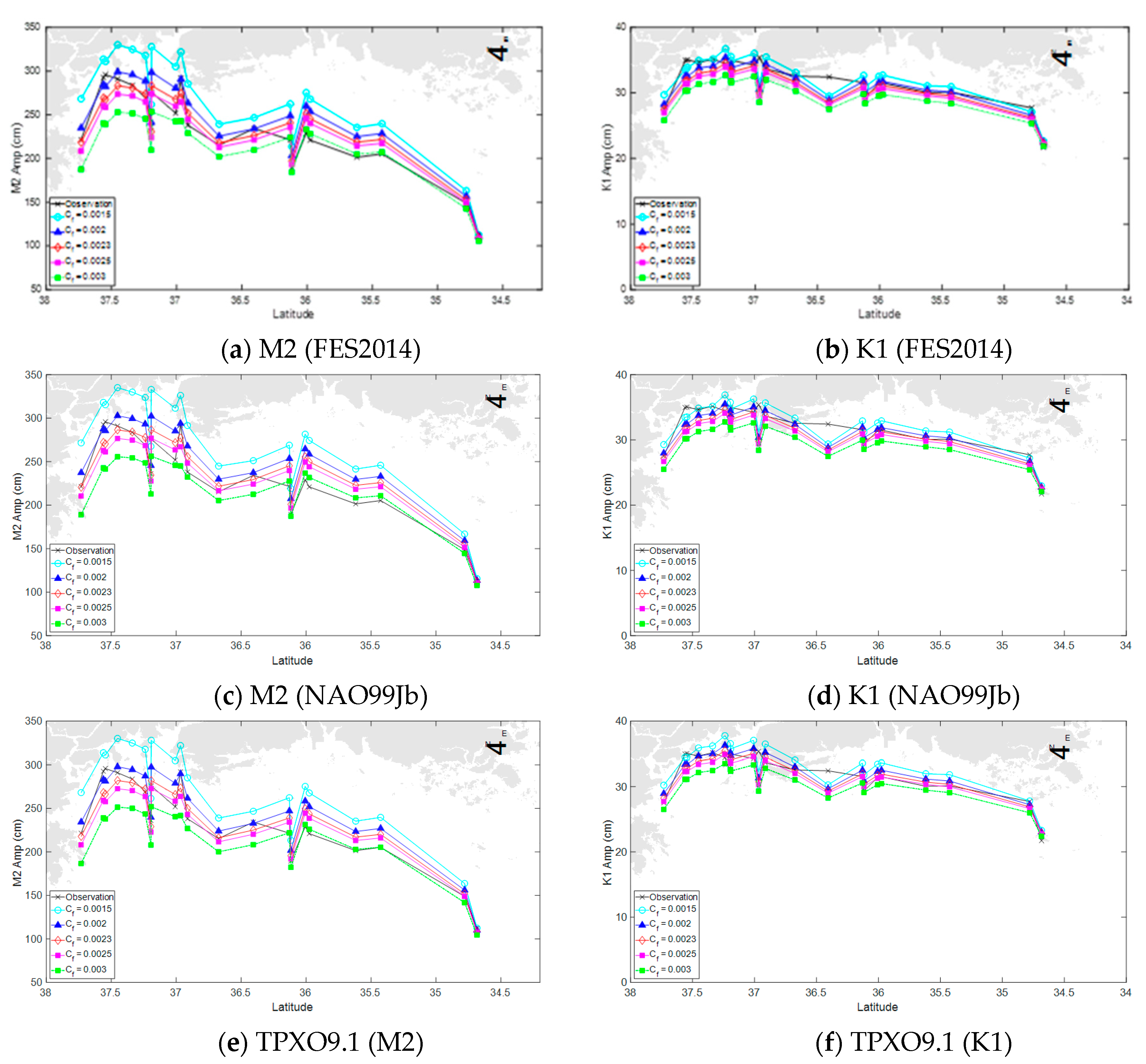
The main goal of this study was to use various numerical investigations to figure out the response of coastal tides in the WCK to the open boundary conditions and bottom roughness. After the application of three different open boundary conditions interpolated from three different assimilated tidal models (FES2014, NAO.99Jb and TPXO9.1), it has been shown that there were no significant differences between the responses of tidal amplitudes in the WCK induced by three open boundary conditions obtained from three assimilated tidal models. In addition, the numerical simulation of the tidal flow in the WCK should not use a uniform bottom roughness coefficient. Due to the complicated bathymetry, indented coastlines and bed variability of the WCK, it caused strong local effects on the tides in this region. Therefore, a non-uniform bottom roughness should be applied to the modeling whereby the smallest value can be applied for Incheon, a larger value for Mokpo, and the largest value for Gunsan. The largest value of the bottom roughness coefficient was applied to the Gunsan region because its bed form was more variable than other regions. The numerical results show that the accuracy of the modeling of the tidal elevation around the WCK was strongly dependent on the bottom roughness rather than the offshore tidal boundary conditions. Moreover, the numerical results can provide not only a better fit to the observations but also higher spatial resolutions in comparison to the results obtained from assimilated tidal models around the WCK.

However, it should be noted that the numerical results obtained from this study were still limited due to the coarse resolution (30 arcs/second) of bathymetry obtained from GEBCO2014, which was not sufficient to capture the real geometries, whose sizes were less than such resolution. Therefore, a further study with a higher resolution is necessary in order to obtain a more precise prediction of the tidal current and its elevation around the WCK. Furthermore, the wind forcing on the sea surface and the tidal energy dissipation should be taken into account.