Assessment of the Water, Environmental, Economic and Social Vulnerability of a Watershed to the Potential Effects of Climate Change and Land Use Change

Abstract
1. Introduction
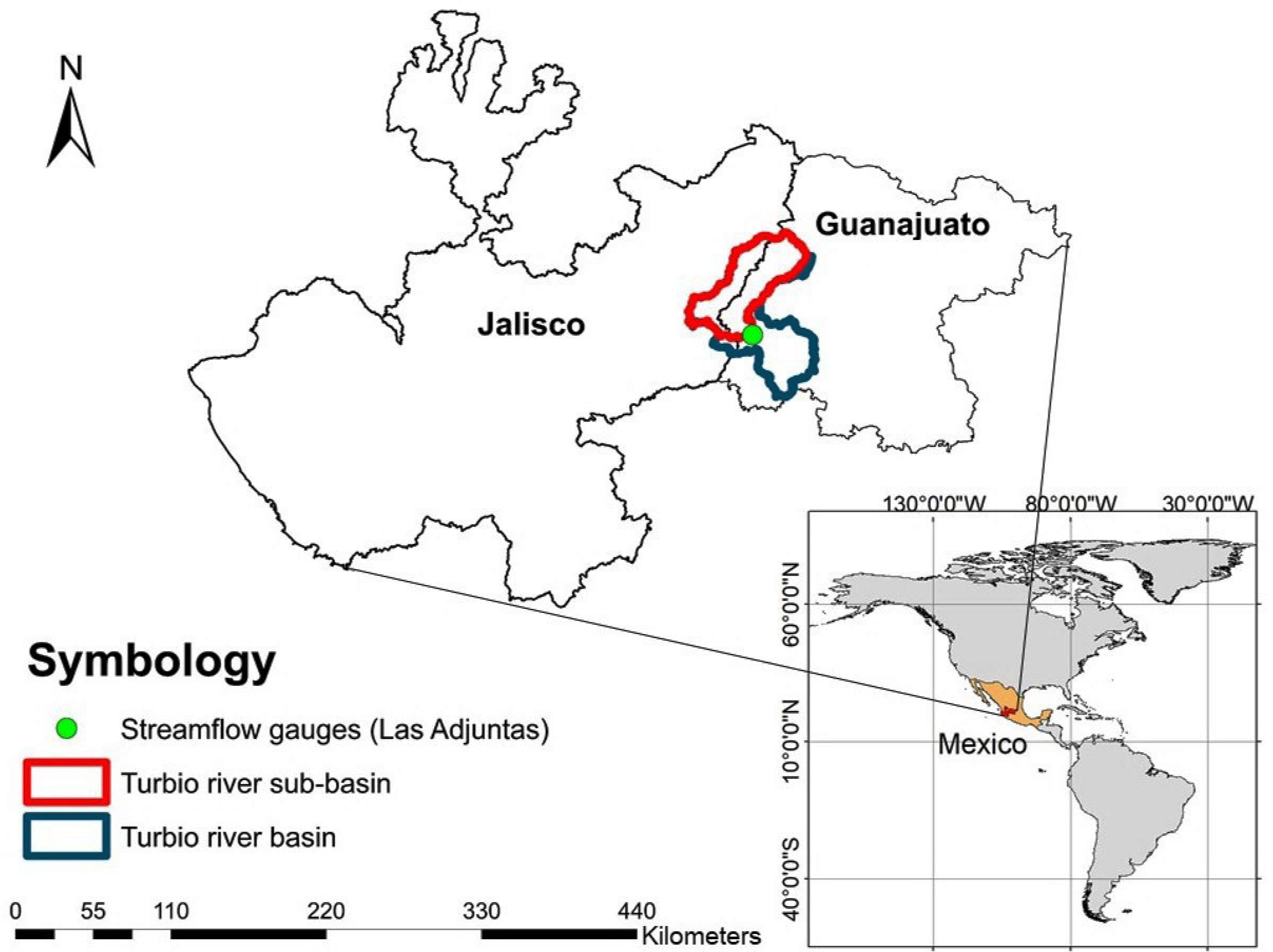
2. Case Study
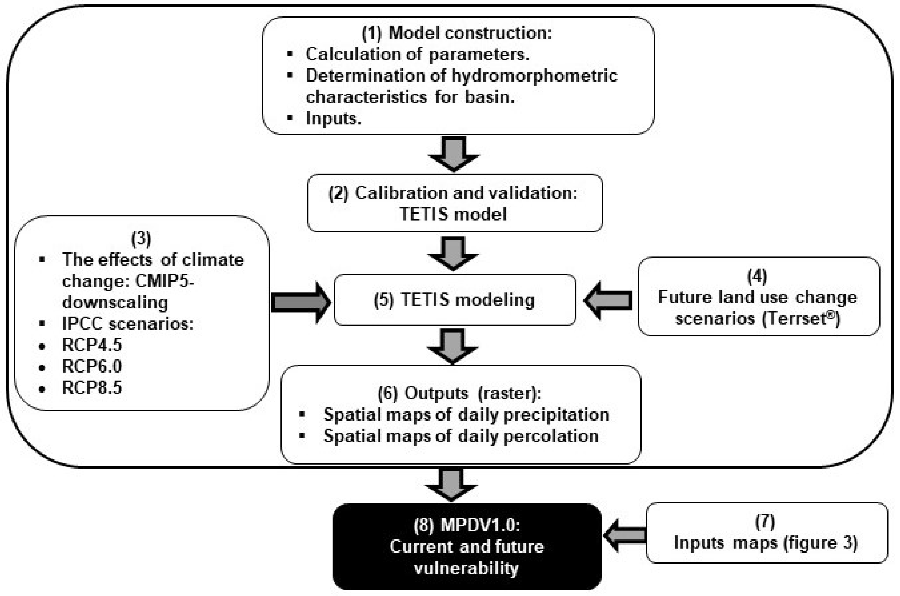
3. Methodology
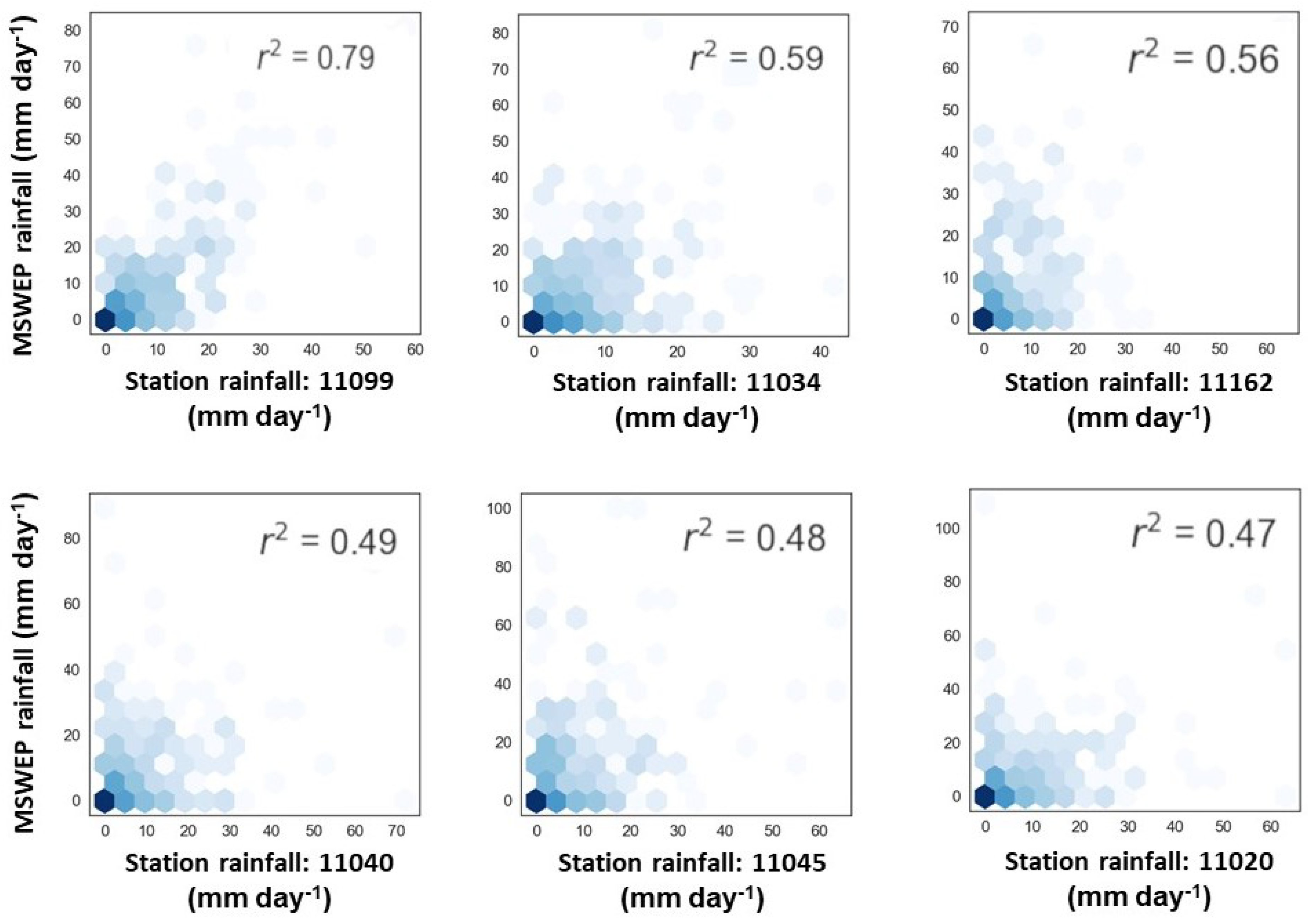
3.1. Data Sets
3.2. Automatic Calibration of the TETIS Model
3.3. Downscaling Climate Model
3.4. Forecast of Land Use Changes
4. Results and Discussion
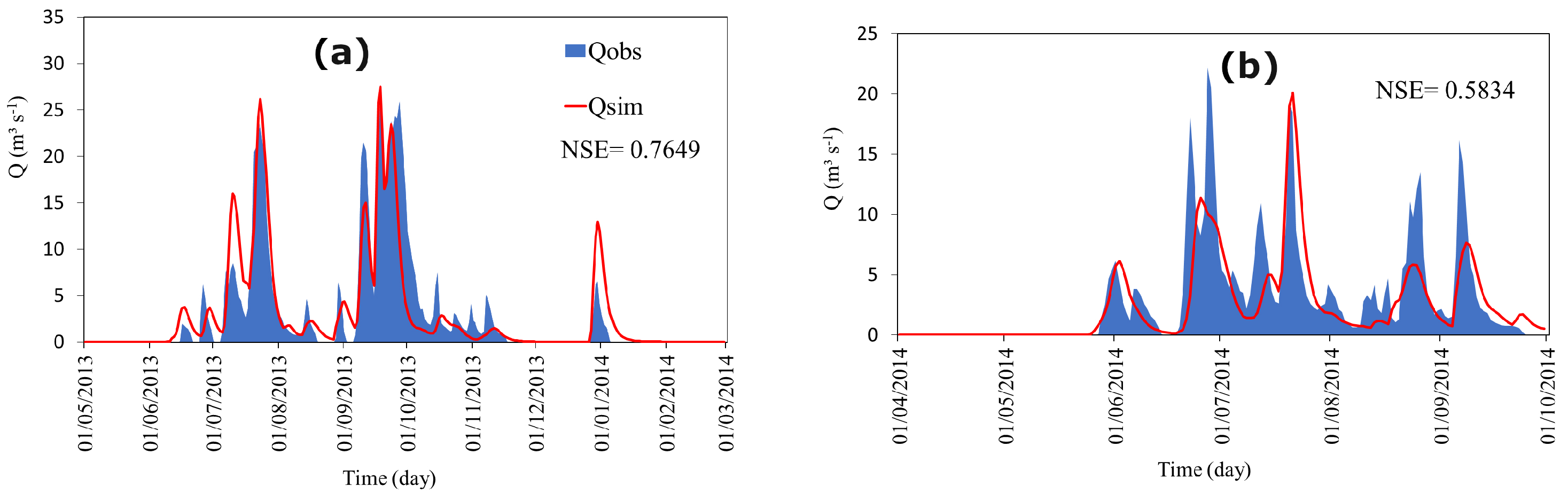
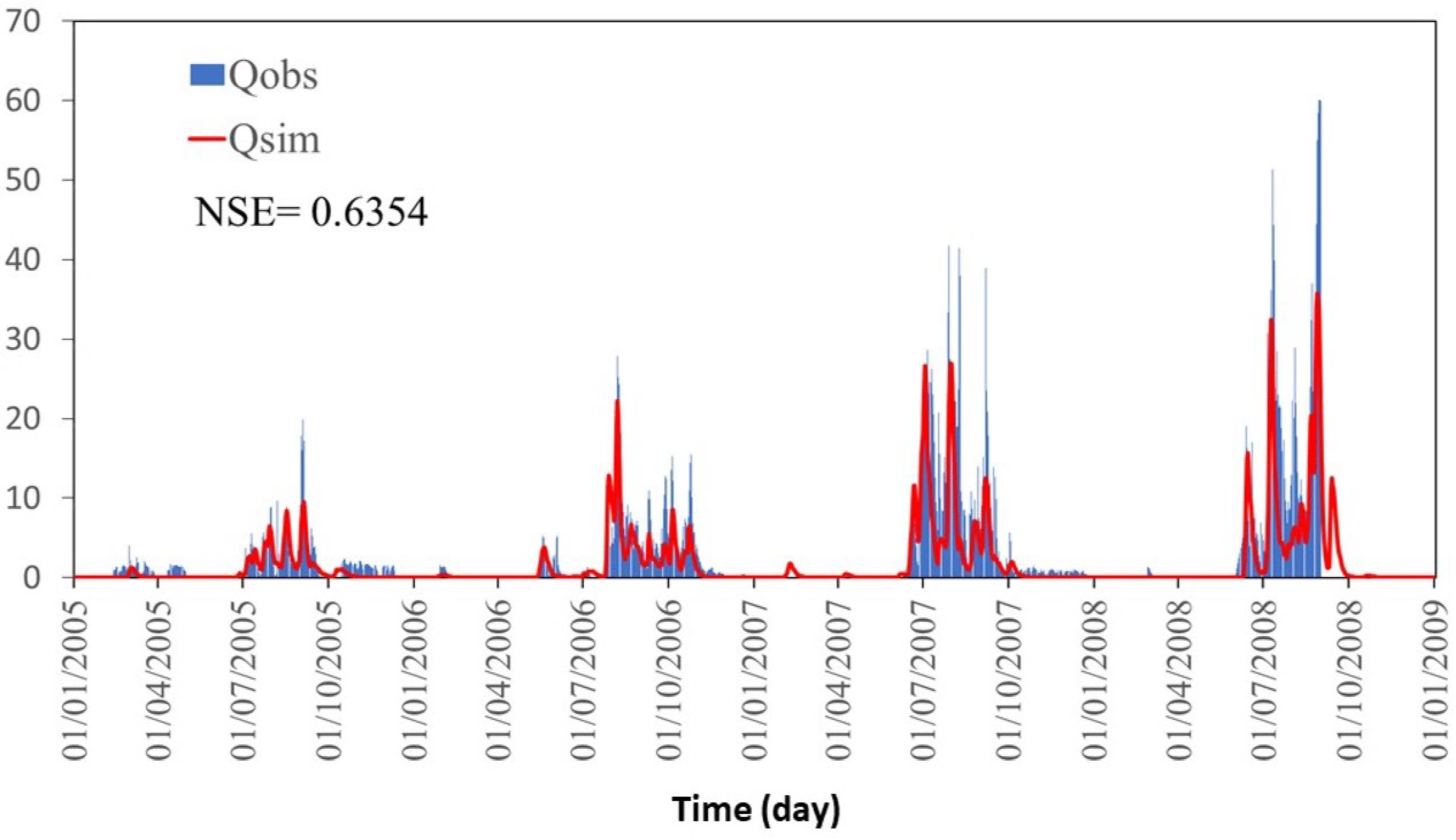
4.1. Hydrology Model Performance
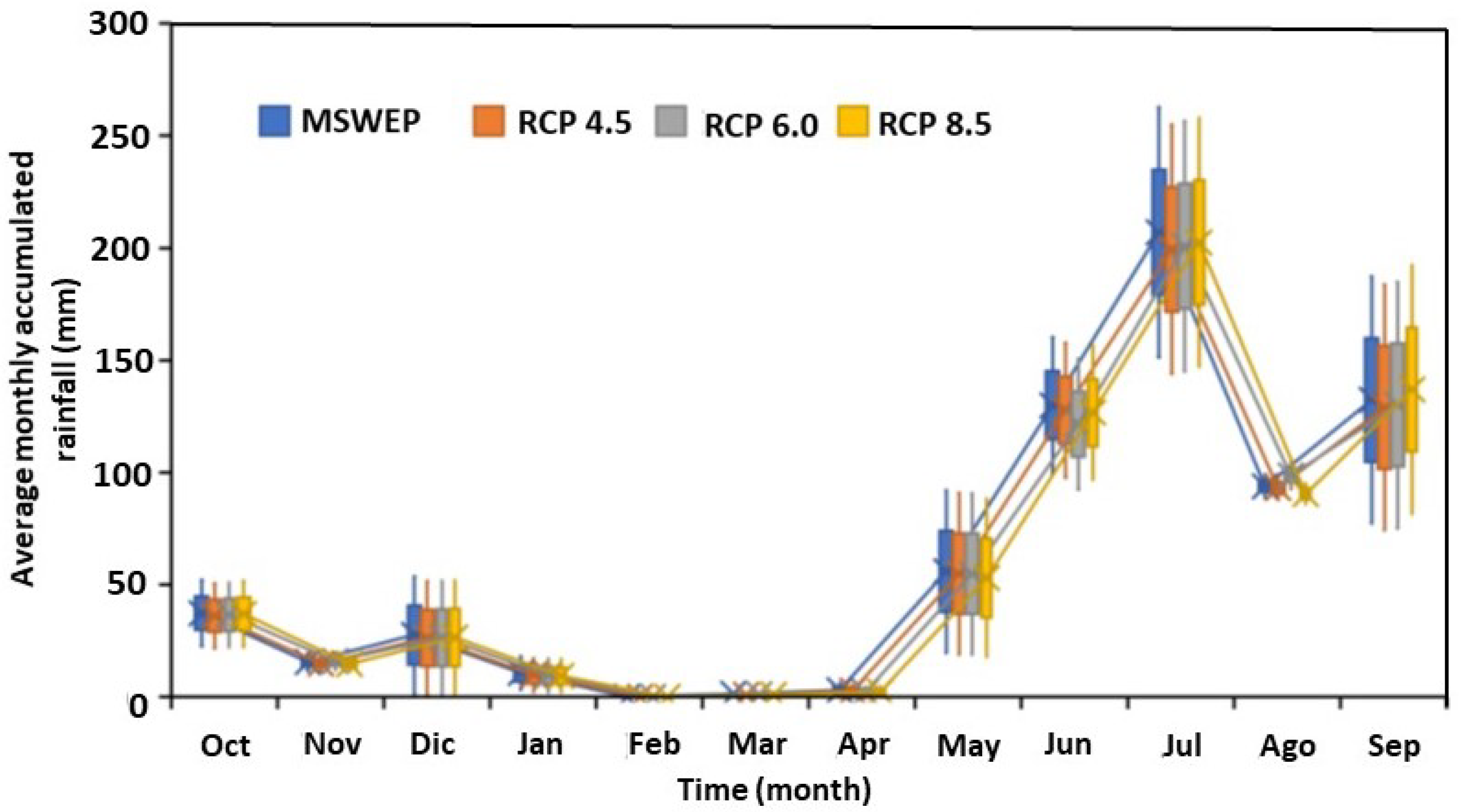
4.2. Climate Projections and Downscaling
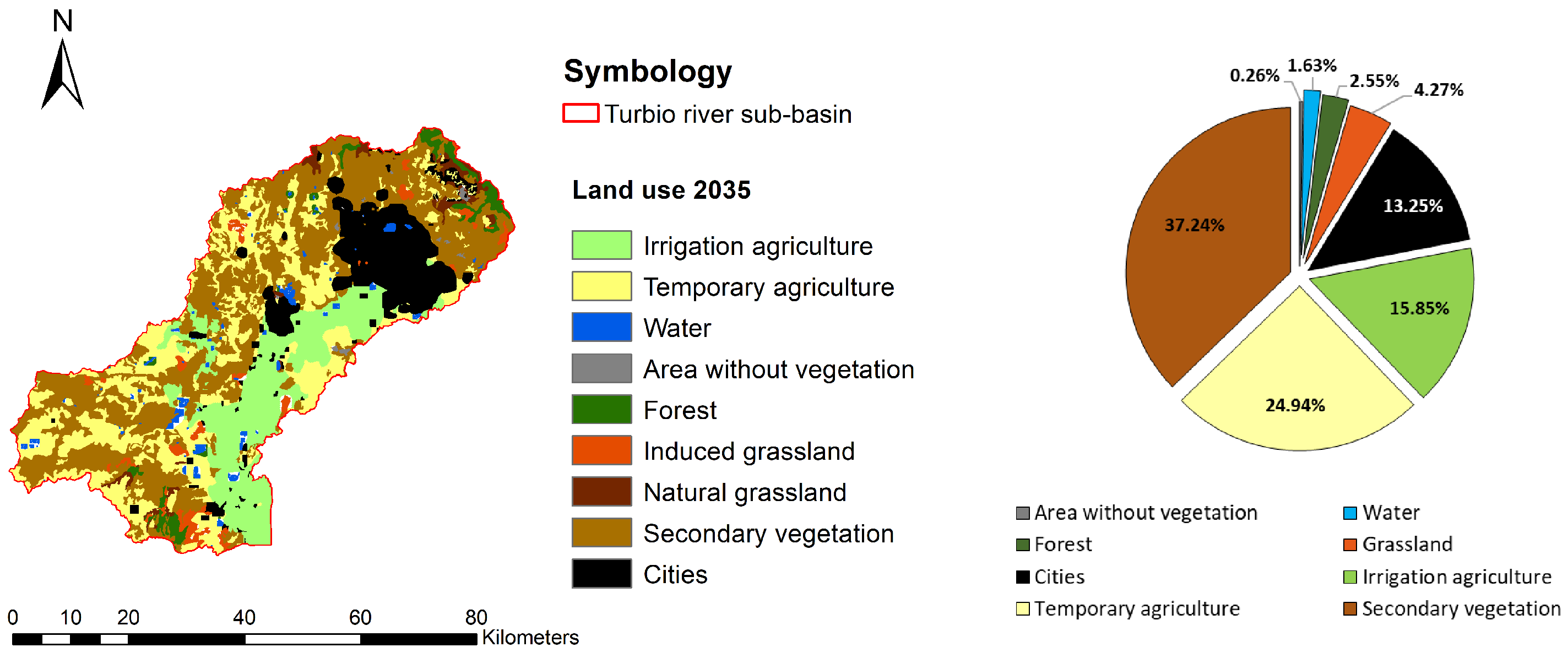
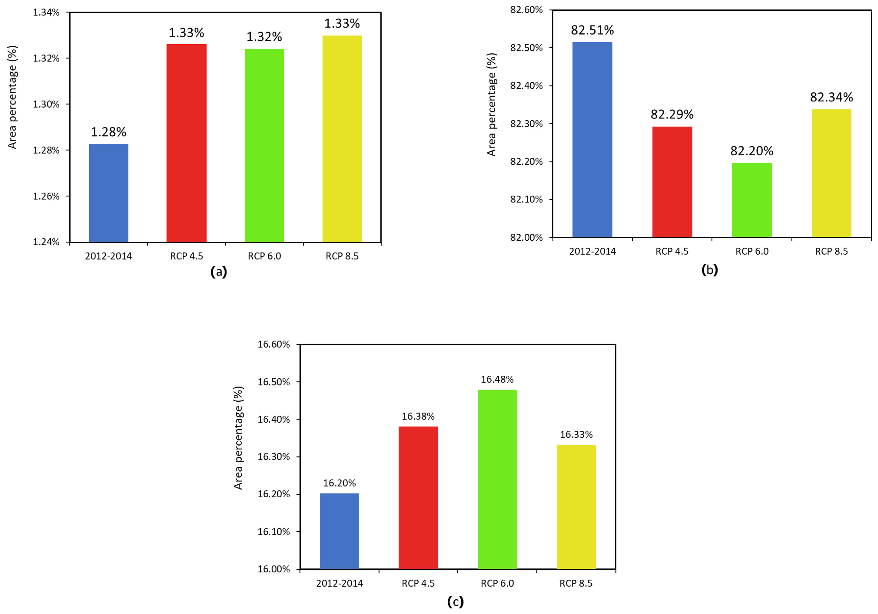
4.3. Future Land Use Change Scenarios Modeling
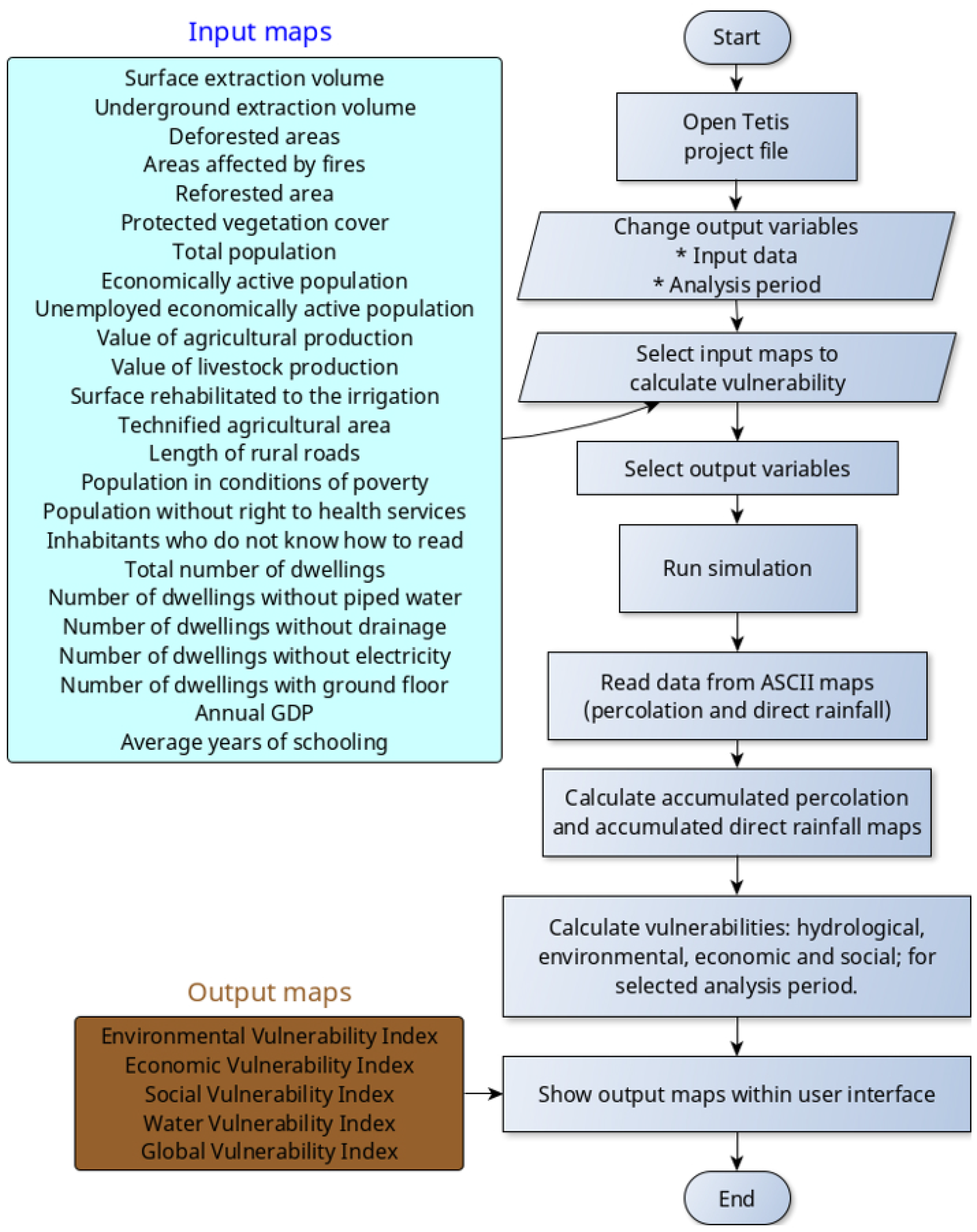
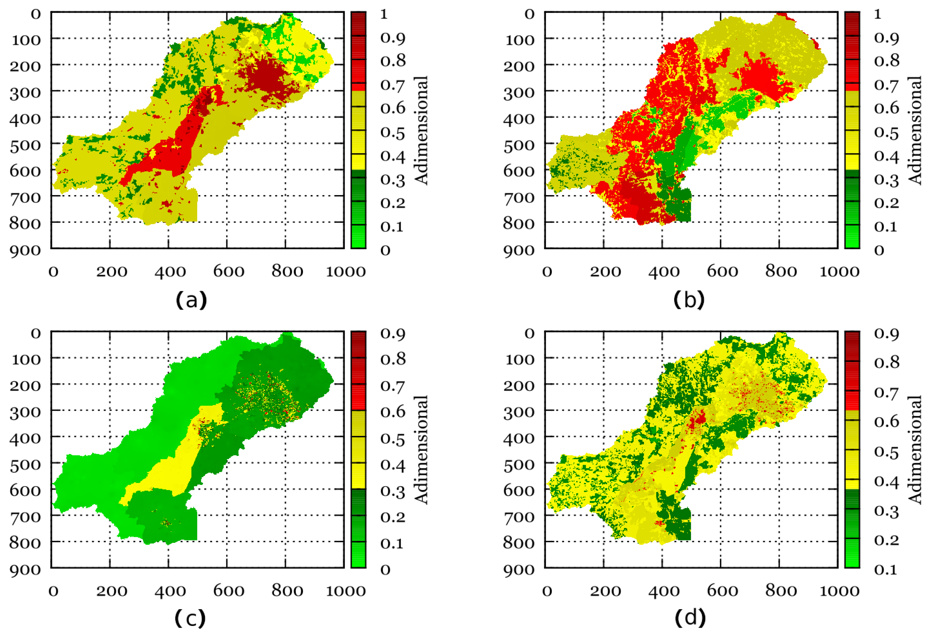
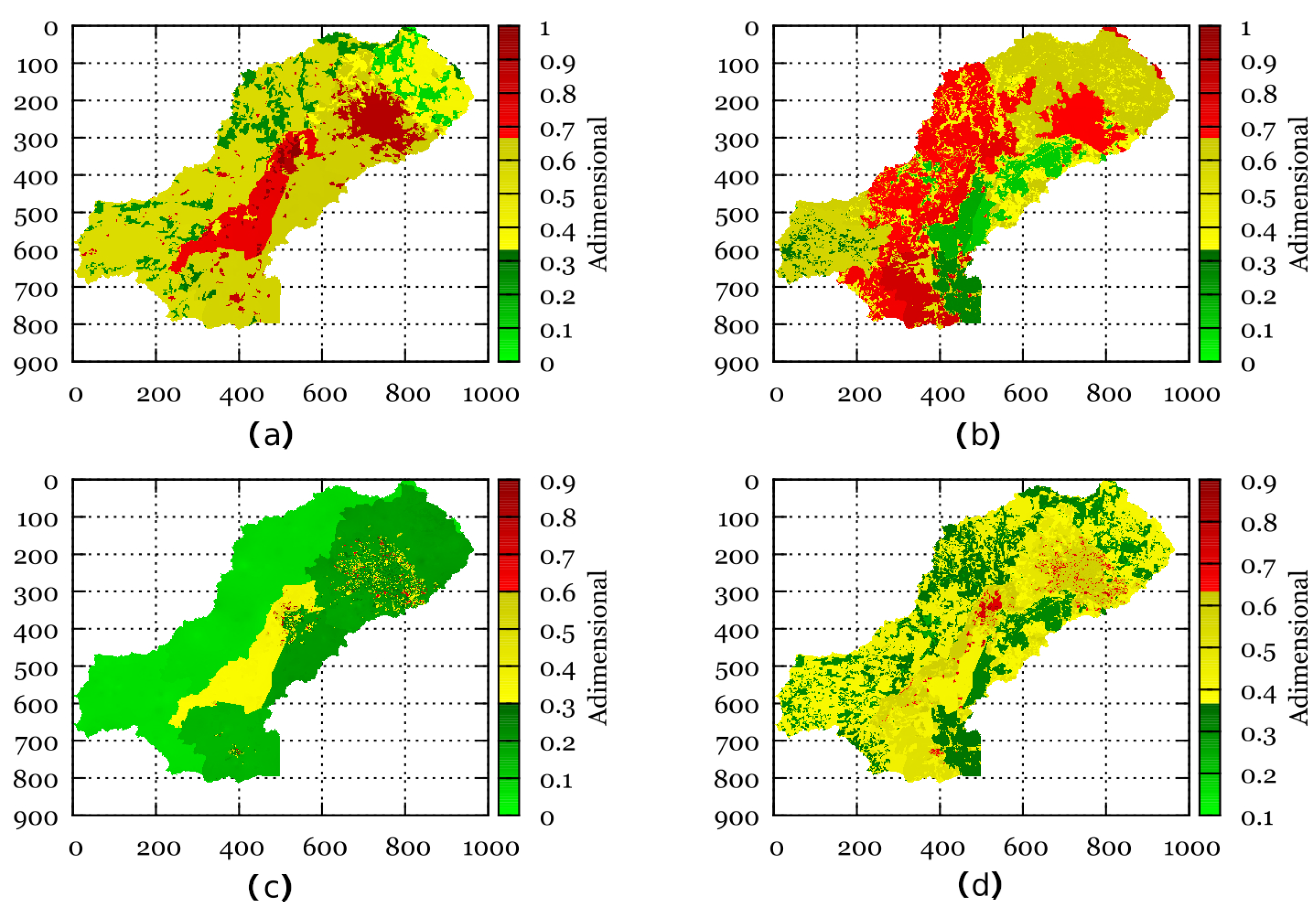
4.4. Assessment of Vulnerability
5. Conclusions
Author Contributions
Funding
Acknowledgments
Conflicts of Interest
References
- Füssel, H.M.; Klein, R.J.T. Climate Change Vulnerability Assessments: An Evolution of Conceptual Thinking. Clim. Chang. 2006, 75, 301–329. [Google Scholar] [CrossRef]
- Parry, M.; Canziani, O.; Palutikof, J.; van der Linden, P.; Hanson, C. Climate Change 2007: Impacts, Adaptation and Vulnerability; Cambridge University Press: Cambridge, UK, 2007. [Google Scholar]
- Hinkel, J. “Indicators of vulnerability and adaptive capacity”: Towards a clarification of the science—Policy interface. Glob. Environ. Chang. 2011, 21, 198–208. [Google Scholar] [CrossRef]
- Marsden, T.; Moragues Faus, A.; Sonnino, R. Reproducing vulnerabilities in agri-food systems: Tracing the links between governance, financialization, and vulnerability in Europe post 2007–2008. J. Agrar. Chang. 2019, 19, 82–100. [Google Scholar] [CrossRef]
- Neset, T.S.; Wiréhn, L.; Opach, T.; Glaas, E.; Linnér, B.O. Evaluation of indicators for agricultural vulnerability to climate change: The case of Swedish agriculture. Ecol. Indic. 2019, 105, 571–580. [Google Scholar] [CrossRef]
- Sujakhu, N.M.; Ranjitkar, S.; He, J.; Schmidt-Vogt, D.; Su, Y.; Xu, J. Assessing the Livelihood Vulnerability of Rural Indigenous Households to Climate Changes in Central Nepal, Himalaya. Sustainability 2019, 11, 2977. [Google Scholar] [CrossRef]
- Bakkensen, L.A.; Fox-Lent, C.; Read, L.K.; Linkov, I. Validating Resilience and Vulnerability Indices in the Context of Natural Disasters. Risk Anal. 2017, 37, 982–1004. [Google Scholar] [CrossRef] [PubMed]
- Tung, C.P.; Tsao, J.H.; Tien, Y.C.; Lin, C.Y.; Jhong, B.C. Development of a Novel Climate Adaptation Algorithm for Climate Risk Assessment. Water 2019, 11, 497. [Google Scholar] [CrossRef]
- Li, L.; Cao, R.; Wei, K.; Wang, W.; Chen, L. Adapting climate change challenge: A new vulnerability assessment framework from the global perspective. J. Clean. Prod. 2019, 217, 216–224. [Google Scholar] [CrossRef]
- Gupta, A.K.; Negi, M.; Nandy, S.; Alatalo, J.M.; Singh, V.; Pandey, R. Assessing the vulnerability of socio-environmental systems to climate change along an altitude gradient in the Indian Himalayas. Ecol. Indic. 2019, 106, 105512. [Google Scholar] [CrossRef]
- Ahsan, M.N.; Warner, J. The socioeconomic vulnerability index: A pragmatic approach for assessing climate change led risks—A case study in the south-western coastal Bangladesh. Int. J. Disaster Risk Reduct. 2014, 8, 32–49. [Google Scholar] [CrossRef]
- Koutroulis, A.; Papadimitriou, L.; Grillakis, M.; Tsanis, I.; Warren, R.; Betts, R. Global water availability under high-end climate change: A vulnerability based assessment. Glob. Planet. Chang. 2019, 175, 52–63. [Google Scholar] [CrossRef]
- Ghimire, S.; Dhungana, N.; Upadhaya, S. Impacts of Climate Change on Water Availability and Reservoir Based Hydropower. J. For. Nat. Resour. Manag. 2019, 1, 52–68. [Google Scholar] [CrossRef]
- Tulbure, M.G.; Broich, M. Spatiotemporal patterns and effects of climate and land use on surface water extent dynamics in a dryland region with three decades of Landsat satellite data. Sci. Total Environ. 2019, 658, 1574–1585. [Google Scholar] [CrossRef] [PubMed]
- Jun, K.S.; Chung, E.S.; Sung, J.Y.; Lee, K.S. Development of spatial water resources vulnerability index considering climate change impacts. Sci. Total Environ. 2011, 409, 5228–5242. [Google Scholar] [CrossRef] [PubMed]
- Hewitson, B.C.; Crane, R.G. Consensus between GCM climate change projections with empirical downscaling: Precipitation downscaling over South Africa. Int. J. Climatol. 2006, 26, 1315–1337. [Google Scholar] [CrossRef]
- Chung, E.S.; Park, K.; Lee, K.S. The relative impacts of climate change and urbanization on the hydrological response of a Korean urban watershed. Hydrol. Process. 2011, 25, 544–560. [Google Scholar] [CrossRef]
- Herrera-Pantoja, M.; Hiscock, K. Projected impacts of climate change on water availability indicators in a semi-arid region of central Mexico. Environ. Sci. Policy 2015, 54, 81–89. [Google Scholar] [CrossRef]
- Wiréhn, L.; Danielsson, Å.; Neset, T.S.S. Assessment of composite index methods for agricultural vulnerability to climate change. J. Environ. Manag. 2015, 156, 70–80. [Google Scholar] [CrossRef]
- Boy-Roura, M.; Nolan, B.T.; Menció, A.; Mas-Pla, J. Regression model for aquifer vulnerability assessment of nitrate pollution in the Osona region (NE Spain). J. Hydrol. 2013, 505, 150–162. [Google Scholar] [CrossRef]
- Abson, D.J.; Dougill, A.J.; Stringer, L.C. Using Principal Component Analysis for information-rich socio-ecological vulnerability mapping in Southern Africa. Appl. Geogr. 2012, 35, 515–524. [Google Scholar] [CrossRef]
- Maiolo, M.; Martirano, G.; Morrone, P.; Pantusa, D. Assessment criteria for a sustainable management of the water resources. Water Pract. Technol. 2006, 1, wpt2006012. [Google Scholar] [CrossRef]
- Tixier, J.; Dandrieux, A.; Dusserre, G.; Bubbico, R.; Mazzarotta, B.; Silvetti, B.; Hubert, E.; Rodrigues, N.; Salvi, O. Environmental vulnerability assessment in the vicinity of an industrial site in the frame of ARAMIS European project. J. Hazard. Mater. 2006, 130, 251–264. [Google Scholar] [CrossRef]
- Lange, H.D.; Sala, S.; Vighi, M.; Faber, J. Ecological vulnerability in risk assessment—A review and perspectives. Sci. Total Environ. 2010, 408, 3871–3879. [Google Scholar] [CrossRef] [PubMed]
- Brody, S.D.; Zahran, S.; Vedlitz, A.; Grover, H. Examining the Relationship Between Physical Vulnerability and Public Perceptions of Global Climate Change in the United States. Environ. Behav. 2008, 40, 72–95. [Google Scholar] [CrossRef]
- Armaş, I.; Gavriş, A. Social vulnerability assessment using spatial multi-criteria analysis (SEVI model) and the Social Vulnerability Index (SoVI model)—A case study for Bucharest, Romania. Nat. Hazards Earth Syst. Sci. 2013, 13, 1481–1499. [Google Scholar] [CrossRef]
- Cheng, J.; Tao, J. Fuzzy Comprehensive Evaluation of Drought Vulnerability Based on the Analytic Hierarchy Process: —An Empirical Study from Xiaogan City in Hubei Province. Agric. Agric. Sci. Procedia 2010, 1, 126–135. [Google Scholar] [CrossRef]
- Manning, L.J.; Hall, J.W.; Fowler, H.J.; Kilsby, C.G.; Tebaldi, C. Using probabilistic climate change information from a multimodel ensemble for water resources assessment. Water Resour. Res. 2009, 45. [Google Scholar] [CrossRef]
- Dixon, B. Applicability of neuro-fuzzy techniques in predicting ground-water vulnerability: A GIS-based sensitivity analysis. J. Hydrol. 2005, 309, 17–38. [Google Scholar] [CrossRef]
- Tang, Z.; Engel, B.; Pijanowski, B.; Lim, K. Forecasting land use change and its environmental impact at a watershed scale. J. Environ. Manag. 2005, 76, 35–45. [Google Scholar] [CrossRef]
- Bai, Y.; Ochuodho, T.O.; Yang, J. Impact of land use and climate change on water-related ecosystem services in Kentucky, USA. Ecol. Indic. 2019, 102, 51–64. [Google Scholar] [CrossRef]
- Quintas-Soriano, C.; Castro, A.J.; Castro, H.; García-Llorente, M. Impacts of land use change on ecosystem services and implications for human well-being in Spanish drylands. Land Use Policy 2016, 54, 534–548. [Google Scholar] [CrossRef]
- Chuai, X.; Huang, X.; Wu, C.; Li, J.; Lu, Q.; Qi, X.; Zhang, M.; Zuo, T.; Lu, J. Land use and ecosystems services value changes and ecological land management in coastal Jiangsu, China. Habitat Int. 2016, 57, 164–174. [Google Scholar] [CrossRef]
- Ruiz-Pérez, G.; González-Sanchis, M.; Campo, A.D.; Francés, F. Can a parsimonious model implemented with satellite data be used for modelling the vegetation dynamics and water cycle in water-controlled environments? Ecol. Model. 2016, 324, 45–53. [Google Scholar] [CrossRef]
- Orozco, I.; Francés, F.; Mora, J. Parsimonious Modeling of Snow Accumulation and Snowmelt Processes in High Mountain Basins. Water 2019, 11, 1288. [Google Scholar] [CrossRef]
- Fazeli Farsani, I.; Farzaneh, M.R.; Besalatpour, A.A.; Salehi, M.H.; Faramarzi, M. Assessment of the impact of climate change on spatiotemporal variability of blue and green water resources under CMIP3 and CMIP5 models in a highly mountainous watershed. Theor. Appl. Climatol. 2019, 136, 169–184. [Google Scholar] [CrossRef]
- Harrison, P.A.; Dunford, R.W.; Holman, I.P.; Cojocaru, G.; Madsen, M.S.; Chen, P.Y.; Pedde, S.; Sandars, D. Differences between low-end and high-end climate change impacts in Europe across multiple sectors. Reg. Environ. Chang. 2019, 19, 695–709. [Google Scholar] [CrossRef]
- Wilson, K.; Newton, A.; Echeverría, C.; Weston, C.; Burgman, M. A vulnerability analysis of the temperate forests of south central Chile. Biol. Conserv. 2005, 122, 9–21. [Google Scholar] [CrossRef]
- Wang, X.; Zhong, X.; Liu, S.; Liu, J.; Wang, Z.; Li, M. Regional assessment of environmental vulnerability in the Tibetan Plateau: Development and application of a new method. J. Arid Environ. 2008, 72, 1929–1939. [Google Scholar] [CrossRef]
- Enea, M.; Salemi, G. Fuzzy approach to the environmental impact evaluation. Ecol. Model. 2001, 136, 131–147. [Google Scholar] [CrossRef]
- Nandy, S.; Singh, C.; Das, K.; Kingma, N.; Kushwaha, S. Environmental vulnerability assessment of eco-development zone of Great Himalayan National Park, Himachal Pradesh, India. Ecol. Indic. 2015, 57, 182–195. [Google Scholar] [CrossRef]
- Altuwaijri, H.A.; Alotaibi, M.H.; Almudlaj, A.M.; Almalki, F.M. Predicting urban growth of Arriyadh city, capital of the Kingdom of Saudi Arabia, using Markov cellular automata in TerrSet geospatial system. Arab. J. Geosci. 2019, 12, 135. [Google Scholar] [CrossRef]
- Managing the Risks of Extreme Events and Disasters to Advance Climate Change Adaptation: Special Report of the Intergovernmental Panel on Climate Change; Cambridge University Press: Cambridge, UK, 2012. [CrossRef]
- Ortega-Gaucin, D.; Bartolón, J.; Castellano, H. Water and Climate Change-Danger, Vulnerability and Risk from Droughts in the Context of Climate Change in Mexico; 2018; pp. 78–101. Available online: https://www.gob.mx/imta/documentos/agua-y-cambio-climatico?idiom=es (accessed on 9 June 2020).
- Beck, H.; Van Dijk, A.; Levizzani, V.; Schellekens, J.; Gonzalez Miralles, D.; Martens, B.; de Roo, A. MSWEP: 3-hourly 0.25° global gridded precipitation (1979–2015) by merging gauge, satellite, and reanalysis data. Hydrol. Earth Syst. Sci. Discuss. 2017, 2, 589–615. [Google Scholar] [CrossRef]
- Alijanian, M.; Rakhshandehroo, G.R.; Mishra, A.K.; Dehghani, M. Evaluation of satellite rainfall climatology using CMORPH, PERSIANN-CDR, PERSIANN, TRMM, MSWEP over Iran. Int. J. Climatol. 2017, 37, 4896–4914. [Google Scholar] [CrossRef]
- Beck, H.E.; Wood, E.F.; Pan, M.; Fisher, C.K.; Miralles, D.G.; van Dijk, A.I.J.M.; McVicar, T.R.; Adler, R.F. MSWEP V2 Global 3-Hourly 0.1° Precipitation: Methodology and Quantitative Assessment. Bull. Am. Meteorol. Soc. 2019, 100, 473–500. [Google Scholar] [CrossRef]
- Prakash, S. Performance assessment of CHIRPS, MSWEP, SM2RAIN-CCI, and TMPA precipitation products across India. J. Hydrol. 2019, 571, 50–59. [Google Scholar] [CrossRef]
- Omranian, E.; Sharif, H.O. Evaluation of the Global Precipitation Measurement (GPM) Satellite Rainfall Products over the Lower Colorado River Basin, Texas. JAWRA J. Am. Water Resour. Assoc. 2018, 54, 882–898. [Google Scholar] [CrossRef]
- Dinku, T.; Chidzambwa, S.; Ceccato, P.; Connor, S.J.; Ropelewski, C.F. Validation of high-resolution satellite rainfall products over complex terrain. Int. J. Remote Sens. 2008, 29, 4097–4110. [Google Scholar] [CrossRef]
- Sun, R.; Yuan, H.; Liu, X.; Jiang, X. Evaluation of the latest satellite–gauge precipitation products and their hydrologic applications over the Huaihe River basin. J. Hydrol. 2016, 536, 302–319. [Google Scholar] [CrossRef]
- Jiang, S.; Ren, L.; Xu, C.Y.; Yong, B.; Yuan, F.; Liu, Y.; Yang, X.; Zeng, X. Statistical and hydrological evaluation of the latest Integrated Multi-satellitE Retrievals for GPM (IMERG) over a midlatitude humid basin in South China. Atmos. Res. 2018, 214, 418–429. [Google Scholar] [CrossRef]
- Francés, F.; Vélez, J.I.; Vélez, J.J. Split-parameter structure for the automatic calibration of distributed hydrological models. J. Hydrol. 2007, 332, 226–240. [Google Scholar] [CrossRef]
- Duan, Q.; Sorooshian, S.; Gupta, V. Effective and efficient global optimization for conceptual rainfall-runoff models. Water Resour. Res. 1992, 28, 1015–1031. [Google Scholar] [CrossRef]
- García-Romero, L.; Paredes-Arquiola, J.; Solera, A.; Belda, E.; Andreu, J.; Sánchez-Quispe, S.T. Optimization of the Multi-Start Strategy of a Direct-Search Algorithm for the Calibration of Rainfall–Runoff Models for Water-Resource Assessment. Water 2019, 11, 1876. [Google Scholar] [CrossRef]
- Bauwe, A.; Eckhardt, K.U.; Lennartz, B. Predicting dissolved reactive phosphorus in tile-drained catchments using a modified SWAT model. Ecohydrol. Hydrobiol. 2019, 19, 198–209. [Google Scholar] [CrossRef]
- Giorgetta, M.A.; Jungclaus, J.; Reick, C.H.; Legutke, S.; Bader, J.; Böttinger, M.; Brovkin, V.; Crueger, T.; Esch, M.; Fieg, K.; et al. Climate and carbon cycle changes from 1850 to 2100 in MPI-ESM simulations for the Coupled Model Intercomparison Project phase 5. J. Adv. Model. Earth Syst. 2013, 5, 572–597. [Google Scholar] [CrossRef]
- Neelin, J.D.; Langenbrunner, B.; Meyerson, J.E.; Hall, A.; Berg, N. California Winter Precipitation Change under Global Warming in the Coupled Model Intercomparison Project Phase 5 Ensemble. J. Clim. 2013, 26, 6238–6256. [Google Scholar] [CrossRef]
- Kusunoki, S.; Arakawa, O. Are CMIP5 Models Better than CMIP3 Models in Simulating Precipitation over East Asia? J. Clim. 2015, 28, 5601–5621. [Google Scholar] [CrossRef]
- Knutti, R.; Sedláček, J. Robustness and uncertainties in the new CMIP5 climate model projections. Nat. Clim. Chang. 2013, 3, 369–373. [Google Scholar] [CrossRef]
- Cavazos, T.; Salinas, J.; Martínez-López, B.; Colorado, G.; Grau, P.; González, R.; Conde, C.; Quintanar, A.; Sepúlveda, J.; Centeno, R.; et al. Actualización de Escenarios de Cambio Climático Para México Como Parte de los Productos de la Quinta Comunicación Nacional; Informe final del proyecto al INECC; Instituto Nacional de Ecología y Cambio Climático: Mexico, Mexico, 2013; p. 150. [Google Scholar]
- Giorgi, F.; Mearns, L.O. Calculation of Average, Uncertainty Range, and Reliability of Regional Climate Changes from AOGCM Simulations via the “Reliability Ensemble Averaging” (REA) Method. J. Clim. 2002, 15, 1141–1158. [Google Scholar] [CrossRef]
- Harris, I.; Jones, P.; Osborn, T.; Lister, D. Updated high-resolution grids of monthly climatic observations – the CRU TS3.10 Dataset. Int. J. Climatol. 2014, 34, 623–642. [Google Scholar] [CrossRef]
- Das, J.; Nanduri, U.V. Assessment and evaluation of potential climate change impact on monsoon flows using machine learning technique over Wainganga River basin, India. Hydrol. Sci. J. 2018, 63, 1020–1046. [Google Scholar] [CrossRef]
- Guan, D.; Li, H.; Inohae, T.; Su, W.; Nagaie, T.; Hokao, K. Modeling urban land use change by the integration of cellular automaton and Markov model. Ecol. Model. 2011, 222, 3761–3772. [Google Scholar] [CrossRef]
- Mas, J.F.; Kolb, M.; Paegelow, M.; Olmedo, M.T.C.; Houet, T. Inductive pattern-based land use/cover change models: A comparison of four software packages. Environ. Model. Softw. 2014, 51, 94–111. [Google Scholar] [CrossRef]
- Halmy, M.W.A.; Gessler, P.E.; Hicke, J.A.; Salem, B.B. Land use/land cover change detection and prediction in the north-western coastal desert of Egypt using Markov-CA. Appl. Geogr. 2015, 63, 101–112. [Google Scholar] [CrossRef]
- Smith, M.; Koren, V.; Zhang, Z.; Moreda, F.; Cui, Z.; Cosgrove, B.; Mizukami, N.; Kitzmiller, D.; Ding, F.; Reed, S.; et al. The distributed model intercomparison project—Phase 2: Experiment design and summary results of the western basin experiments. J. Hydrol. 2013, 507, 300–329. [Google Scholar] [CrossRef]
- Moriasi, D.N.; Arnold, J.G.; Van Liew, M.W.; Bingner, R.L.; Harmel, R.D.; Veith, T.L. Model Evaluation Guidelines for Systematic Quantification of Accuracy in Watershed Simulations. Trans. ASABE 2007, 50, 885–900. [Google Scholar] [CrossRef]
- Freitas, L.; Afonso, M.J.; Pereira, A.J.S.C.; Delerue-Matos, C.; Chaminé, H.I. Assessment of sustainability of groundwater in urban areas (Porto, NW Portugal): A GIS mapping approach to evaluate vulnerability, infiltration and recharge. Environ. Earth Sci. 2019, 78, 140. [Google Scholar] [CrossRef]
- Okadera, T.; Wang, Q.X.; Deni, E.; Nakayama, T. Groundwater monitoring for evaluating the pasture carrying capacity and its vulnerability in arid and semi-arid regions: A case study of urban and mining areas in Mongolia. IOP Conf. Ser. Earth Environ. Sci. 2019, 266, 012013. [Google Scholar] [CrossRef]
- Dinpashoh, Y.; Jahanbakhsh Asl, S.; Rasouli, A.; Singh, V. Impact of climate change on potential evapotranspiration (case study: West and NW of Iran). Theor. Appl. Climatol. 2018, 136, 185–201. [Google Scholar] [CrossRef]
- Doglioni, A.; Simeone, V. Effects of Climatic Changes on Groundwater Availability in a Semi-arid Mediterranean Region. In IAEG/AEG Annual Meeting Proceedings, San Francisco, California, 2018—Volume 4; Shakoor, A., Cato, K., Eds.; Springer International Publishing: Cham, Switzerland, 2019; pp. 105–110. [Google Scholar]


| Vulnerability | Indicator (Equation and Units) | |
|---|---|---|
| Global | Economic | Population density (PD): ; (hab km) |
| Economically active population (EAP): ; | ||
| Length of rural roads (LRR): ; (km) | ||
| Economic value of agricultural production (EAP): ; (thousand of pesos) | ||
| Economic value of the cattle industry (ECI): ; (thousand of pesos) | ||
| Agricultural area for irrigation (AAI): ; (ha) | ||
| Agriculture area with technified irrigation (ATI): ; (ha) | ||
| Social | Population without medical services (PWMS): ; | |
| Population in poverty (PP): ; | ||
| Illiterate population (IP): ; | ||
| Houses without drinking water (HDW): ; | ||
| Houses without drainage and no restroom (HDR): ; | ||
| Houses without electricity (HWE): ; | ||
| Houses with land floor (HLF): ; | ||
| Per capita anual net income (PCI): ; | ||
| Beneficiaries of the social program: opportunities (BPO): ; | ||
| Beneficiaries of the social program: Liconsa (BPL): ; | ||
| Environmental | Degree of exploitation of the basin (DEB): ; (adimensional) | |
| Degree of exploitation of groundwater (DEG): ; (adimensional) | ||
| Deforestation (DEF): ; | ||
| Area affected by forest fires (AFF): ; | ||
| Reforested surface (RS): ; (ha) | ||
| Protected natural areas (ANP): ; | ||
| Water | Degree of exploitation of the basin (DEB): ; (adimensional) | |
| Degree of exploitation of groundwater (DEG): ; (adimensional) | ||
| Model | Institution | Country |
|---|---|---|
| BBC-CSM1 | Beijing Climate Center, China Meteorological Administration | China |
| MIROC-ESM-CHEM, MIROC-ESM and MIROC5 | Atmosphere and Ocean Research Institute, National Institute for Environmental Studies and Japan Agency for Marine-Earth Science and Technology | Japan |
| CanESM2 | Canadian Centre for Climate Modelling and Analysis | Canada |
| CNRMCM5 | Centre National de Recherches Météorologiques-Centre Européen de Recherche et de Formation Avancée en Calcul Scientifique | France |
| CSIRO-MK3-6 | Commonwealth Scientific and Industrial Research Organisation | Australia |
| GFDL_CM3 | Geophysical Fluid Dynamics Laboratory | USA |
| GISS-E2-R | National Aeronautics and Space Administration Goddard Institute for Space Studies | USA |
| HADGEM2-Es | Met Office Hadley Centre | UK |
| INM-CM4 | Mathematical center | Russia |
| MPI-ESM-LR | Max Planck Institute for Meteorology | Germany |
| MRI-CGCM3 | Meteorological Research Institute | Japan |
| NCC-NorESM1 | Bjerknes Centre for Climate Research and Norwegian Meteorological Institute | Norway |
| IPSL-CMA-LR | Institut Pierre-Simon Laplace | France |
| Parameter | Correction Factor | Parameter Equation | Effective Parameter |
|---|---|---|---|
| Static storage | = 0.677 | 340.83 (mm) | |
| Vegetation cover index | = 0.500 | 3.34 (-) | |
| Infiltration capacity | = 0.814 | 0.35 (mm h) | |
| Overland flow velocity | = 0.850 | 2.64 (m s) | |
| Percolation capacity | = 250.00 | 0.16 (mm h) | |
| Interflow velocity | = 0.010 | 0.003 (mm h) | |
| Deep aquifer permeability | = 200.00 | 0.045 (mm h) | |
| Connected aquifer permeability | = 0.001 | 0.003 (mm h) | |
| River channel velocity | = 0.131 | 0.187 (mm s) |
| IPCC Scenario | Period | Control Period 1982–2014 (mm) | Annual Average Accumulated Rainfall Forecast (mm) | Rainfall Variations (mm) |
|---|---|---|---|---|
| RCP 4.5 | 2015–2039 | 656.4 | 620.4 | −36.1 |
| RCP 6.0 | 2015–2039 | 656.4 | 621.1 | −35.4 |
| RCP 8.5 | 2015–2039 | 656.4 | 623.8 | −32.6 |
| Variable | CMIP5-IPCC Projections (Period:2015–2039) | ||
|---|---|---|---|
| RCP4.5 | RCP6.0 | RCP8.5 | |
| Temperature (°C) | 2.5 | 2.4 | 2.6 |
© 2020 by the authors. Licensee MDPI, Basel, Switzerland. This article is an open access article distributed under the terms and conditions of the Creative Commons Attribution (CC BY) license (http://creativecommons.org/licenses/by/4.0/).
Share and Cite
Orozco, I.; Martínez, A.; Ortega, V. Assessment of the Water, Environmental, Economic and Social Vulnerability of a Watershed to the Potential Effects of Climate Change and Land Use Change. Water 2020, 12, 1682. https://doi.org/10.3390/w12061682
Orozco I, Martínez A, Ortega V. Assessment of the Water, Environmental, Economic and Social Vulnerability of a Watershed to the Potential Effects of Climate Change and Land Use Change. Water. 2020; 12(6):1682. https://doi.org/10.3390/w12061682
Chicago/Turabian StyleOrozco, Ismael, Adrián Martínez, and Víctor Ortega. 2020. "Assessment of the Water, Environmental, Economic and Social Vulnerability of a Watershed to the Potential Effects of Climate Change and Land Use Change" Water 12, no. 6: 1682. https://doi.org/10.3390/w12061682
APA StyleOrozco, I., Martínez, A., & Ortega, V. (2020). Assessment of the Water, Environmental, Economic and Social Vulnerability of a Watershed to the Potential Effects of Climate Change and Land Use Change. Water, 12(6), 1682. https://doi.org/10.3390/w12061682