Multivariate Monitoring of Surface Water Quality: Physico-Chemical, Microbiological and 3D Fluorescence Characterization

Abstract

The primary objective of this study is to explore a water quality database on two Mediterranean rivers (the Kadisha-Abou Ali and El Jaouz rivers—located in north Lebanon), considering their physicochemical, microbiological and fluorescence characteristics. Principal Component Analysis (PCA) was applied to the matrix gathering physicochemical and microbiological data while the Common Components and Specific Weight Analysis (CCSWA) or ComDim was used for fluorescence excitation-emission matrices (EEMs). This approach provided complementary and valuable information regarding water quality in such complex ecosystem. As highlighted by the PCA and ComDim scores, the Kadisha-Abou Ali River is highly influenced by anthropogenic activities because its watershed districts are intensively populated. This influence reveals the implication of organic and bacteriological parameters. To the contrary, the El Jaouz watershed is less inhabited and is characterized by mineral parameters, which determines its water quality. This work highlighted the relationship between fluorescence EEMs and major water quality parameters, enabling the selection of reliable water quality indicators for the studied rivers. The proposed methodology can surely be generalized to the monitoring of surface water quality in other rivers. Each customized water quality fingerprint should constantly be inspected in order to account for any emerging pollution.

1. Introduction

Many aquatic ecosystems in the world undergo continuous stress, which might represent a serious threat for water resources and public health. Many international instances rushed to take actions to raise awareness towards this serious problem. Among them, the water action decade (2018–2028) is currently one of the main goals of the United Nations sustainable development goals [1]. To preserve the integrity of these aquatic ecosystems, water management programs should be established. It is, however, obvious that no remarkable progress can be achieved in the absence of criteria, which would uncontestably allow the monitoring of water quality.

Currently, the term “water quality” is a fuzzy concept, which hinders the establishment of reliable monitoring tools. In fact, before seeking suitable methodologies for its evaluation, it is necessary to first define water quality. Although this problem is mentioned frequently in the literature [2,3,4,5] at the present time, it remains an unsettled issue which led to the introduction of the concept of “water mass reference”. The only solution that seems acceptable is that each type of water should constitute its own reference. This approach leads to a comprehension of the state of a water body relative to a defined situation at a defined time and place; this water will then act as its own relative reference [6].

In order to define the water mass reference for a water body, generally, several quality parameters are measured. These include physico-chemical and microbiological quality variables [6]. Moreover, some spectroscopic techniques have been developed, enabling fast, simple and non-destructive characterization of water samples like UV [7] and fluorescence spectroscopy [8,9,10]. Furthermore, samples are generally collected at different sampling sites and during multiple time periods. This spatiotemporal analysis combined with the different quality variables generates complex data sets enclosing, in some cases, three-dimensional data as in the case of fluorescence excitation-emission matrices (EEMs) [10,11].

To solve this problem, multivariate approaches are employed. Principal Component Analysis (PCA) seems preferable [12] in the case of two-dimensional (2D) data matrices, normally gathering physico-chemical and microbiological parameters [13,14,15]. However, PCA is too often regarded as a simple tool of description or reduction of the dimensionality. Nevertheless, when PCA is appropriately used, it allows the generation of a multivariate fingerprint, defining a water mass reference and thus enabling the development of an assessment tool for water quality monitoring. Besides unsupervised tools, predictive modeling is also gaining much attention in this field, like the PLS-PM analysis [16], enabling to push further the applicability of multivariate approaches towards predicting the ecological status of aquatic ecosystems in the near future. For three-dimensional (3D) data, such as fluorescence EEMs, several approaches have been proposed to better understand the organic matter composition of surface water. The most popular tool remains the parallel factor analysis (PARAFAC), which allows the decomposition of the fluorescence signal into underlying individual fluorescent phenomena while respecting the trilinear nature of fluorescence data [8,9,10,11]. However, another interesting tool has been developed for multiblock data analysis, called the Common Components and Specific Weight analysis (CCSWA) or ComDim, standing for Common Dimensions [17]. ComDim assesses the relationships between samples and variables within a multiblock setting, where several variables, organized in blocks, are measured on the same sample [18]. In the case of EEMs, the blocks could be defined according to emission wavelengths or excitation wavelengths allowing the treatment of such 3D data [19].

In this study, multivariate methodologies were applied to monitor two rivers in North Lebanon (Kadisha-Abou Ali and El Jaouz rivers). PCA was implemented to exploit matrices gathering physico-chemical and microbiological parameters, whereas, ComDim was applied on fluorescence EEMs. To our knowledge, no published work on the use of ComDim for the evaluation of surface water fluorescence data has been reported yet. The overall goal of this research is to provide insight into the relationship between fluorescence EEMs and major water quality indicators, enabling the selection of reliable water fingerprints to define a river water mass reference.

2. Materials and Methods

2.1. Study Area

In the present study, data was collected from the Kadisha—Abou Ali and El Jaouz rivers, located in North Lebanon (Figure 1). These two rivers flow westward to reach the Mediterranean Sea. Both river basins are adjacent and are largely constituted of limestone. These rivers have similar geomorphological and climatic characteristics but support different human impacts. In fact, human agglomerations and activities (more industrialized) in the Kadisha-Abou Ali basin are remarkably concentrated and intense at the riverbank, which is not the case for the El Jaouz River, where human activities are primarily agricultural, and the human agglomerations are spread all over the basin area. The geomorphological variations (drastic changes in topography in only several kilometers from the coast to the mountains), as well as the climatic variations (rain and snow in winter and dryness in summer), impart to these Mediterranean system specificities proper to this region. Kadisha-Abou Ali and El Jaouz are perennial rivers characterized by high water velocity due to an accentuated slope, with maximum flow rates being recorded in March and April. Minimum flows are typically recorded in September and October [20].

The Kadisha-Abou Ali River originates in Kadisha’s cave (1850 meters above the sea level), flows through the Kadisha Valley and reaches the sea at Tripoli. This river’s length is approximately 45 km, and its average annual flow is 369 Mm³/year (average 15.17 m³/s, max 37.3 m³/s, min 1.6 m³/s), which constitutes approximately 7 to 12% of the total annual average flow of Lebanese surface water in general [21,22].

The El Jaouz River, which primarily originates from sources of Jroud Tannourine, runs out at a distance of 32.3 km with an average annual discharge rate of 76 Mm³/year (average 2.4 m³/s, max 6.18 m³/s, min 0.4 m³/s) to reach the Mediterranean Sea at Koubba—Batroun [20].

Based on the hydrological and topographic river features, six monitoring stations on the Kadisha-Abou Ali River (designated from KA1 to KA6) and eight monitoring stations on the El Jaouz River (designated from J7 to J14) were selected (Figure 1). The monitoring sites were selected according to their interest for the study (point and/or non-point sources of pollution and human activities) and based on the accessibility of the site due to the steep slopes of the two river basins. Supplementary Materials Table S1 describes some geographical characteristics of these sites.

2.2. Sampling and Analytical Procedures

Twenty-six monitoring campaigns were performed, covering a year and a half, extending from July 2003 to December 2004. For the Kadisha-Abou Ali River, another sampling campaign was performed, 7 years after, during the year 2010–2011. Five stations were sampled, corresponding to stations KA1 to KA5. This data set was already published in Daou et al. [6] and was used in this study for comparison and validation purposes.

For physicochemical analyses, the sampled water was transported in two 1-L polyethylene bottles, previously washed and cleaned with deionized water. For microbiological analyses, the samples were collected in 500-mL glass bottles, previously washed and sterilized by autoclave. Thirty physicochemical and microbiological parameters were measured following standard and recommended methods [23] (

Table 1. List of studied parameters and methods applied for measurement.

Parameters	Abbreviation	Method	Parameters	Abbreviation	Method
Temperature (°C)	T°	Potentiometer HORIBA U10	Chemical oxygen demand (mg O2/L)	COD	NF T 90-101
pH	pH	Potentiometer HORIBA U10	Alkalinity (meq/L)	TA	NF T 90-036
Conductivity (µS/cm)	EC	Potentiometer HORIBA U10	Chloride (mg Cl−/L)	Cl	NF T90-014
Dissolved Oxygen (mg O2/L)	DO	Potentiometer HORIBA U10	Total count (CFU/100 mL)	TotGerms	NF T 90-401
Turbidity (NTU)	Turb	Potentiometer HORIBA U10	Total Coliforms (CFU/100 mL)	TotColif	NF T 90-414
Redox (mV, H)	E	Potentiometer WTW pH 330 i	Fecal Coliforms (CFU/100 mL)	FecColif	NF T 90-414
Suspended Solids (mg/L)	SS	NF T 90-105	Fecal Streptococci (CFU/100 mL)	StrepD	NF T 90-416
Orthophosphate (µg P/L)	PO4	NF T 90-023	Sodium (mg/L)	Na	ICP
Total Phosphorus (µg P/L)	P	NF T 90-023	Calcium (mg/L)	Ca	ICP
Nitrates (mg NO3−/L)	NO3	NF T 90-045	Potassium (mg/L)	K	ICP
N ammonia (mg N/L)	NH4	NF T 90-015	Magnesium (mg/L)	Mg	ICP
UV Absorbance at 254 nm	Abs254	Spectrophotometry UV/visible	Iron (µg/L)	Fe	ICP
Sulfates (mg SO42−/L)	SO4	NF T 90-009	Manganese (µg/L)	Mn	ICP
Silicates (mg SiO2/L)	SiO2	NF T 90-007	Barium (µg/L)	Ba	ICP
Dissolved organic carbon (mg C/L)	DOC	Shimadzu TOC-VCSH	Aluminum (µg/L)	Al	ICP

ICP = Inductively Coupled Plasma, Perkin Elmer, Optima 4300 DV, NF = Normes Francaises (French Standards).

).

Fluorescence 3D spectra were acquired on water samples, previously acidified and filtered, using a Jobin Yvon HORIBA ISA Spex Fluoromax 2 spectrofluorometer (Jobin Yvon Spex, Edison, NY, USA). Excitation–emission matrices (EEMs) were recorded as a set of emission spectra between 300 and 550 nm and at excitation wavelengths ranging between 200 and 450 nm, implying 25 excitation and 101 emission wavelength values. All samples were blank corrected using ultra-pure water.

2.3. Multivariate Analyses

First, several descriptive statistics (minimum and maximum values, mean and standard deviation) were calculated for the data set, and Pearson correlations for the different studied parameters of the two rivers were also evaluated (SPSS statistics software package version 22, IBM, Armonk, NY, USA).

Second, a PCA was performed on the matrix gathering physico-chemical and bacteriological parameters using the SPSS statistics software package (version 22), while the ComDim implementation in the SAISIR toolbox [24] was applied on fluorescence EEMs using MATLAB version R2016a (The MathWorks, Natick, MA, USA).

2.3.1. Principal Component Analysis (PCA)

PCA is a powerful technique designed to transform the original variables of a data set into new, uncorrelated variables (orthogonal axes), called the principal components (PC), which are linear combinations of the original variables [25,26]. The new axes lie along the directions of maximum variance. This technique starts with a correlation matrix describing the dispersion of the original variables (measured parameters) and extracting the eigenvalues and eigenvectors. An eigenvector is a list of coefficients (loadings or weightings) by which the original correlated variables are multiplied to obtain the principal components. A principal component is the product of the original data and an eigenvector; the result of projecting the data onto a new axis is a new variable. There are, as many PCs as original variables; however, PC provides information on the most meaningful parameters, which describe the entire dataset, yielding data reduction with minimum loss of original information. In this study, PCA was applied to a data set including 364 samples (14 sampling locations × 26 sampling campaigns) × 30 physico-chemical and microbiological variables, after column standardization (mean centering each variable and dividing the resulting values by the column’s standard deviation). Various preliminary tests, such as the Kaiser, Meyer and Olkin index (KMO) and Bartlett tests were performed to examine the appropriateness of the data for PCA analysis.

2.3.2. ComDim Method

ComDim is a particular implementation of the “Common Components and Specific Weights Analysis” (CCSWA) procedure [27,28,29]. ComDim determines a common space describing the dispersion among data sets or blocks through sample scores; each block having a specific weight or “salience” associated with each dimension in this common space, the Common Components (CCs). Significant differences in the values of saliences for a given dimension reflect the fact that the dimension contains different amounts of information from each block. In addition, and for each CC, the ComDim procedure calculates the loadings of the variables in each block, enabling further interpretation of the highlighted discriminations [28]. Here, ComDim was applied on the 3D array (173 samples × 25 excitation wavelengths × 101 emission wavelengths), which was treated as 101 blocks or matrices corresponding to the emission wavelengths. The 173 samples corresponded to the 14 sampling locations along Kadisha-Abou Ali and El Jaouz rivers, sampled between July and February, thus covering 14 sampling campaigns.

3. Results and Discussions

The summary of the minima, maxima and mean values, as well as the standard deviations of the measured variables in both river water samples, for the complete seasons, are attached as Supplementary Materials Tables S2 and S3. This will provide readers with an overview of the descriptive database of the two studied rivers.

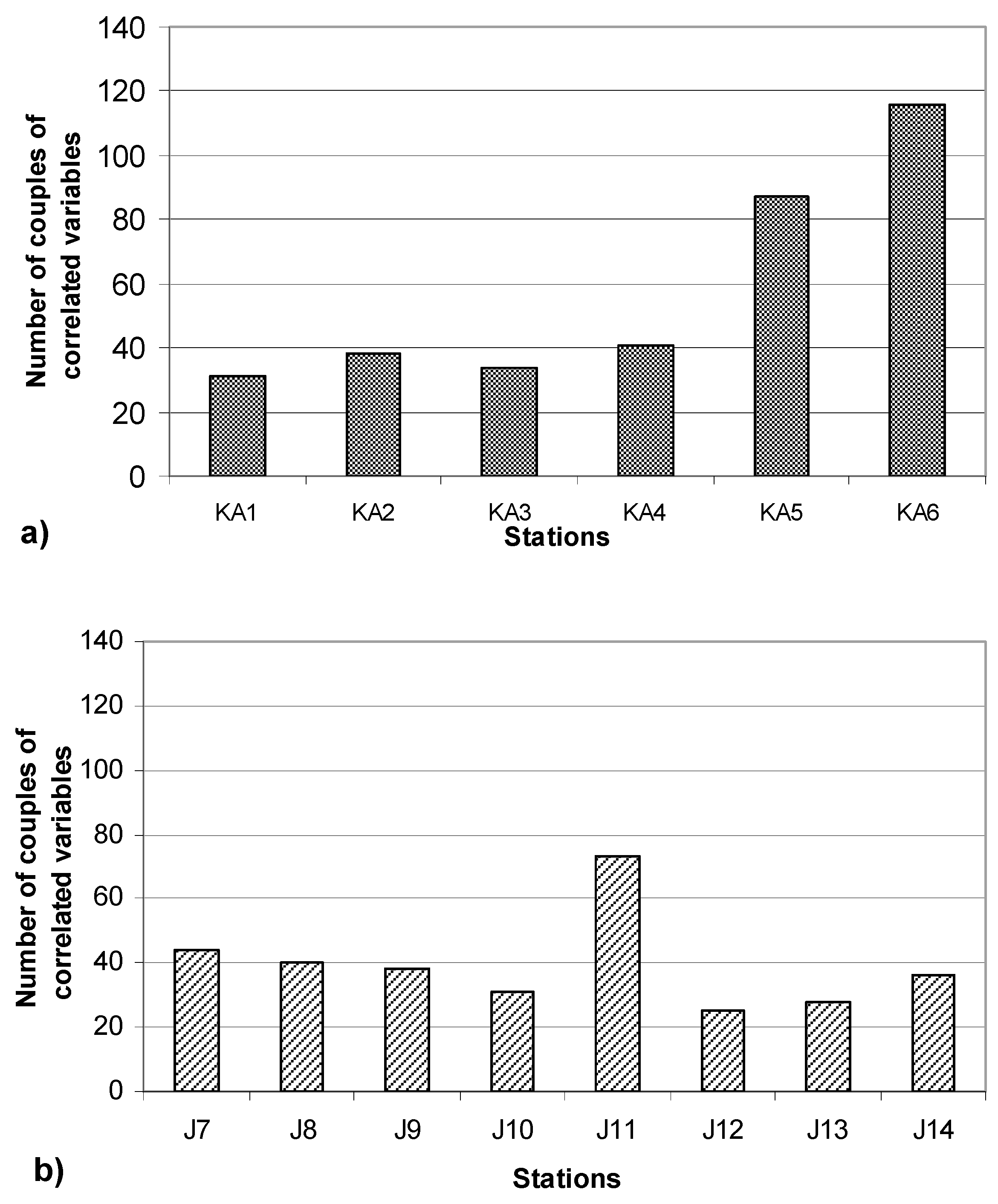
3.1. Study of Bivariate Correlations

The correlations between parameters’ couples were studied using Pearson coefficient method (R). Considering 435 sets of coupled variables present in the correlation matrix [(302-30)/2], the frequencies of the coupled variables with Pearson coefficients higher than 0.5 are presented in Figure 2, for each site. In fact, these correlation coefficients can be simultaneously affected by spatial and temporal variations [30]. In this study, a site-variable correlation matrix was selected in order to evaluate spatial variations of the considered variables. Moreover, we assume that, after the introduction of any anthropogenic disturbance, the aquatic ecosystem attempts to create or modify the chemical bonds between the different parameters. In that way, by reestablishing the equilibrium generated by physicochemical and biological processes, the response to the disturbance is immediate. The number as well as the intensity of the bivariate correlations must therefore be modified (generally increased) by any aquatic ecosystem pollution.

Concerning the Kadisha-Abou Ali River, the results presented in Figure 2a show that the number of correlations having R higher than 0.5 increased for the sites KA2, KA5 and KA6. This finding is due to the wastewater discharge impact of the Tourza agglomeration at site KA2, and the strongly anthropogenic disturbance from the Tripoli agglomeration at sites KA5 and KA6. The same trend has been already described in our previous study on the Kadisha-Abou Ali River [6]. Moreover, Varol [31] reported a decreasing trend of correlations of certain parameters like TSS, COD, NH4-N, Na and K due to anthropogenic activities, highlighting the link between anthropogenic disturbances and the number of correlated variables. Concerning the El Jaouz River (Figure 2b), a higher number of significant correlations is observed for site J11, a site-variable correlation as described by the same study [31]. This finding is probably due to the agricultural activities located in the Kfarhelda agricultural area, which may contribute to the eutrophication process increased by the natural deceleration of the water mass flow in this highland area. For the El Jaouz River, the results do not follow, as we would generally expect, an increasing progression in the upstream-downstream direction. If one considers the dispersion of the human activities along the river basins, slopes and the processes of self-purification, this observation does not seem abnormal.

3.2. Multivariate Study of Water Characteristics

Two different multivariate techniques are applied here to understand the factors that influence surface water quality in the two studied watersheds. This approach will provide valuable tools for interpreting such large dataset and building a multivariate model allowing the definition of the water mass references for the two studied rivers. First, PCA was used to interpret the interactions between the physicochemical and/or microbiological parameters [5]. To reduce the dimensionality of our dataset and to be able to compare the water quality of the different river sites [15], several PCAs were applied to our database (14 samples × 30 parameters × 26 sampling campaigns). Second, ComDim was applied to assess organic matter composition through fluorescence properties of these watersheds, since their characteristics may reflect the water quality in aquatic ecosystems [32].

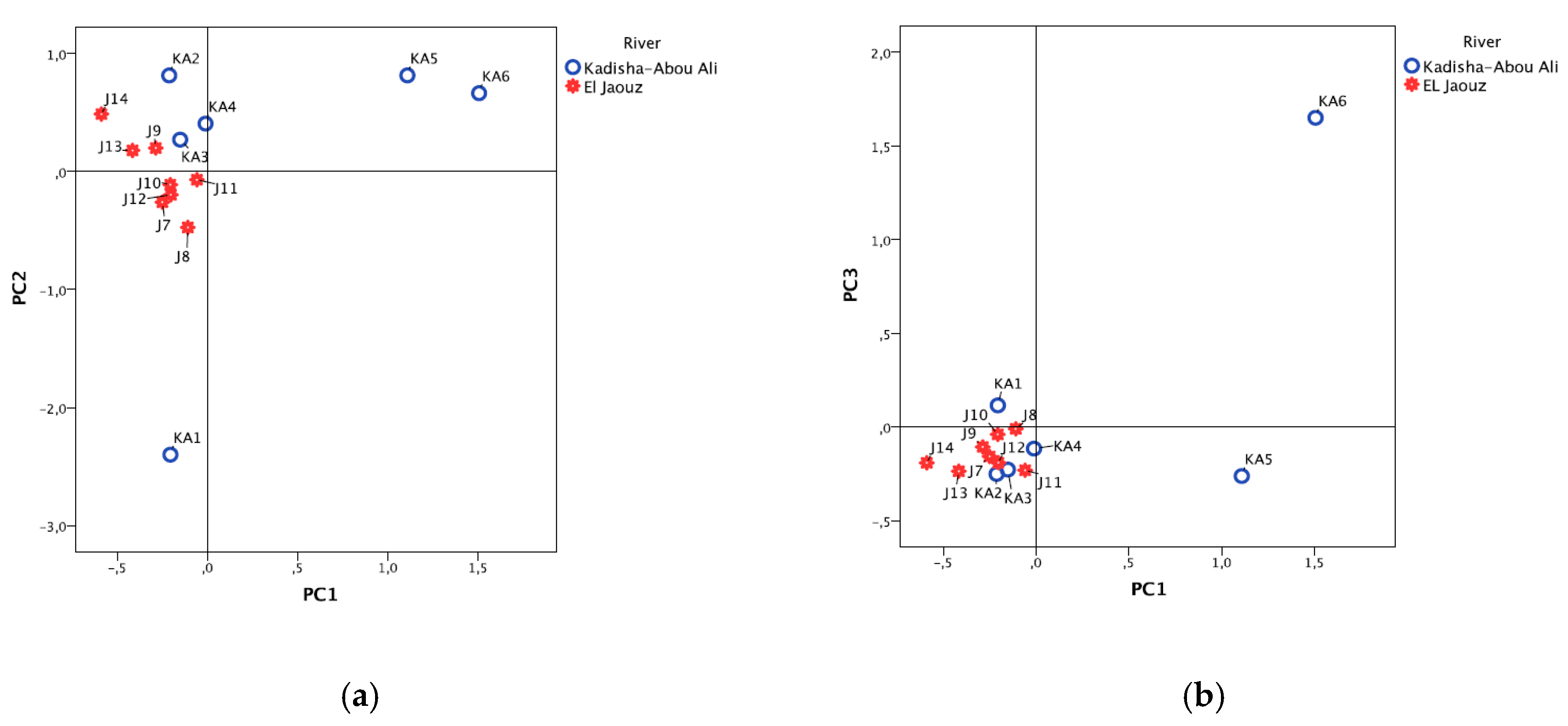
3.2.1. Spatial Study by PCA—The Two Rivers, all Sites, All Parameters

For this PCA, the preliminary tests were adequate (KMO = 0.847 and significance level = 0), indicating the presence of significant relationships between the variables [13]. Insofar, as they are satisfactory, these tests will not be further presented. Supplementary Materials Table S4 shows the explained variances for the six extracted components, which explain a relatively significant portion of the total dataset variance. The variable “loadings” are presented in

Table 2. Matrix of the first six components obtained for the general Principal Component Analysis (PCA) applied to the data matrix including the two rivers, all variables and all sites.

Variable	Component
	1	2	3	4	5	6
Abs254	0.875	0.088	0.183	0.039	0.032	0.037
NH4	0.786	0.144	0.228	0.263	−0.018	−0.034
DOC	0.759	0.160	0.237	−0.058	0.089	−0.038
K	0.704	0.444	0.357	0.194	0.088	0.097
SS	0.623	0.126	0.104	0.169	0.128	0.128
Mn	0.611	0.186	0.198	0.178	0.488	0.105
Na	0.554	0.509	0.420	0.343	−0.014	0.058
Mg	0.019	0.825	0.032	−0.087	0.103	0.023
Ca	0.255	0.790	0.156	0.206	0.103	−0.036
EC	0.171	0.673	0.269	0.395	−0.017	−0.188
TA	0.316	0.639	−0.047	0.119	−0.186	−0.002
T°	0.139	0.638	0.229	0.086	0.063	−0.483
SiO2	0.086	0.628	0.180	0.123	0.024	0.203
SO4	0.383	0.520	−0.023	-0.036	0.013	0.517
Cl	0.456	0.479	0.241	0.466	0.012	−0.050
TotColif	0.151	0.150	0.941	0.104	0.017	0.050
StrepD	0.159	0.084	0.876	0.066	0.042	0.058
FecColif	0.283	0.102	0.820	0.130	−0.008	0.043
TotGerms	0.414	0.117	0.738	0.143	0.045	0.095
Turb	0.108	0.242	0.283	0.240	0.097	−0.001
pH	−0.004	0.050	0.040	−0.730	0.066	−0.161
COD	0.136	0.134	0.187	0.685	0.041	0.030
Ba	0.234	0.266	0.179	0.587	-0.077	−0.182
E	−0.179	−0.214	−0.135	−0.308	-0.009	0.290
Al	0.048	0.008	−0.014	−0.074	0.963	−0.012
Fe	0.165	0.031	0.044	−0.021	0.961	−0.001
DO	−0.031	−0.209	0.030	−0.038	0.049	0.773
NO3	0.123	0.392	0.178	0.356	0.012	0.522
P	0.141	0.146	0.334	0.032	−0.033	0.472
PO4	0.313	0.259	0.328	0.253	−0.053	0.382

. The most significant correlations are highlighted, i.e., those which contribute the most to the construction of the components.

According to Table 2, the first component primarily describes the anthropogenic water characteristics, comprising higher loadings for Abs254, DOC, NH₄ and Mn. The second component describes the mineral water characteristics primarily related to the rock substrate (EC, Na, Ca, Mg and TA), as well as the climatic conditions (T°). The characteristics of these first two components have been already observed in previous studies [13,16,26,33,34,35]. More precisely, Bouza-Deaño et al. [30] and Marinović Ruždjak and Ruždjak [36] reported that the first and forth components presented mineral (geogenic) and anthropogenic characteristics, respectively. The third component exclusively describes the variables defining the microbiological parameters. A similar result was highlighted by Razmkhah et al. [33], where the third component in the PCA conducted on their overall database was described solely by total and fecal coliforms, contributing to the organic pollutions of their watershed. Component 5 describes minor elements and component 6 is defined by the agricultural impacts. These findings demonstrate that there are generally few links between the organic and mineral characteristics of the water. The fact that component 3 only describes the microbiological water quality also shows the weak links between the physicochemical (specifying by that, the mineral parameters) and the microbiological parameters. The microbial contamination could be logically more associated to organic and nutrient variables originated from municipal and industrial point-source discharges, agricultural non-point sources, livestock operations and/or domestic sources [13].

For all PC scores, the choice was to represent the barycenter of all the spatiotemporal data, which differentiates each site. The first PCA shows that the two rivers are well discriminated in the PC1-PC2 plot and, in particular, the sites KA1, KA5 and KA6 of the Kadisha-Abou Ali River (Figure 3a). The other sites of the same river (KA2, KA3 and KA4) are located close to those of the El Jaouz River, indicating that their water has relatively similar characteristics. Site KA6 is discriminated by strong organic characteristics, primarily related to the anthropogenic inputs of Tripoli but also by certain mineral parameters. These mineral characteristics cannot in this case be only linked to the watershed substrate. A considerable part comes from the anthropogenic inputs. Site KA5 has strong mineral characteristics probably also due to anthropogenic origins. This site has less pronounced organic characteristics than site KA6 but stronger than the other sites. That finding is partly due to the organic and mineral inputs of the industrial activities of the suburbs of Tripoli.

Site KA1 has low mineral characteristics (negative quadrant of PC2), as well as low organic characteristics (negative quadrant of PC1). One could assign this water as the “water mass reference” for the studied river, taking into consideration the very low anthropogenic inputs from its location at the head of the catchment area. The same observation was highlighted by Zheng et al. [37], where they found that the site located in the headwater of the Nenjiang River in China had an optimal water quality due to limited human activities. Ustaoğlu et al. [38] reported that the upstream site of the Turnasuyu stream in Turkey was separated from other stations in the dendrogram obtained from the cluster analysis. Karakaya and Evrendilek [39] also reported a significant difference between upstream and downstream stations of the Melen River in Turkey, and variables revealed a significant water quality degradation along the upstream-to-downstream gradient due to pollution input from point and non-point sources. In fact, the midstream and downstream of the Melen River were similar to each other, while the upstream station was different. Once more, these observations show a large extent of similarities with our study, where an upstream-downstream degradation of water quality was highlighted for the Kadisha-Abou Ali River. The position of the downstream sites (KA2, KA3 and KA4) on the PC plot regarding this general approach seems to indicate that their water quality is rather similar. However, a specific analysis of only these sites will be able to highlight the differences in quality, which exist between them. Considering the scores plot, specifically PC1-PC3 (Figure 3b), a very clear discrimination of site KA6 can be noticed based on the bacteriological water quality (position on PC3). The decrease of physicochemical water quality at this site is accompanied by a drastic degradation of the microbiological quality. In a study on the same river [21], it was also reported that Tripoli station (corresponding to KA6 in our study) is highly polluted mainly due to direct sewage discharge. Thus, the conditions for bacterial growth were favorite in summer where the water flow is relatively slow (0.8 m³/s). To the contrary, at the other sites, discrimination from the microbiological point of view does not appear evident. That finding is due to the “collapsing” effect with respect of the PC plot of site KA6 and, to a certain extent, of site KA5. The characteristics of this water, from its very large anthropogenic stress are very different from the others, which in comparison appear to be of similar quality.

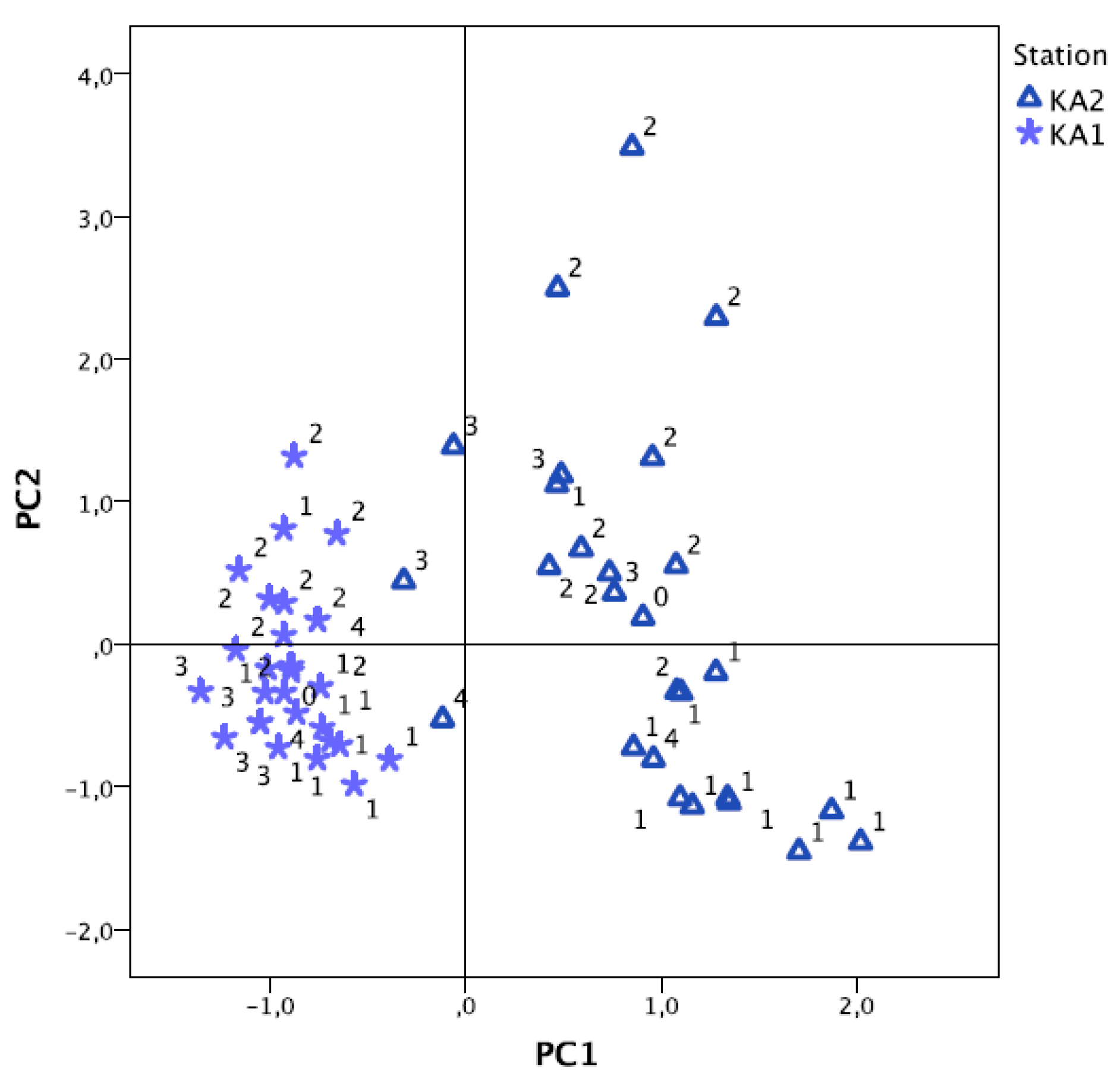
3.2.2. Spatial Study by PCA—The Two Rivers, All Variables, Excluding Sites KA5 and KA6

To better understand the ambiguity caused by the very disparate water quality of sites KA5 and KA6, a solution could be to perform a new PCA without these two sites. This approach was already tested in our previous work on the Arka River [14].

Table 3. Matrix of the first six components obtained for the PCA applied to the data matrix including the two rivers, all variables and all sites excluding KA5 and KA6.

Variable	Component
	1	2	3	4	5	6
Mg	0.802	0.092	−0.004	0.023	0.248	0.083
Ca	0.801	0.138	−0.004	0.038	0.036	−0.025
Na	0.798	−0.017	0.341	0.067	−0.212	0.073
EC	0.777	−0.026	−0.123	0.107	−0.197	−0.148
TA	0.740	−0.107	0.111	−0.030	0.084	−0.005
K	0.668	0.221	0.357	0.075	0.297	0.126
Cl	0.647	0.051	−0.092	0.076	0.089	−0.255
T°	0.605	0.055	−0.585	0.030	0.176	0.143
E	−0.335	0.059	0.002	0.050	0.273	−0.074
Turb	0.317	0.100	0.076	0.194	−0.110	0.074
Fe	0.007	0.951	−0.008	−0.001	−0.028	0.063
Al	0.015	0.931	0.003	0.000	−0.065	0.072
Mn	0.098	0.792	0.004	−0.001	0.130	0.055
DO	−0.265	0.072	0.745	−0.076	0.168	−0.167
PO4	0.041	−0.055	0.566	−0.075	0.129	0.094
SO4	0.434	0.049	0.527	0.053	0.318	0.052
NH4	0.087	−0.053	0.496	0.322	−0.202	0.142
SS	0.194	0.261	0.405	0.306	0.031	0.038
FecColif	0.297	−0.121	0.319	0.217	−0.066	0.133
TotColif	0.080	−0.021	0.015	0.935	0.062	0.034
StrepD	−0.001	0.010	0.021	0.890	0.107	−0.064
P	−0.131	−0.064	0.171	−0.053	0.616	0.085
Ba	0.324	−0.137	0.058	0.162	−0.518	−0.303
NO3	0.226	0.054	0.456	0.057	0.509	−0.291
SiO2	0.408	−0.019	−0.047	0.039	0.500	−0.180
TotGerms	0.110	−0.002	0.046	0.171	0.337	−0.015
pH	−0.007	0.074	0.030	0.047	0.005	0.721
DOC	0.125	−0.011	0.001	0.123	0.093	−0.599
COD	0.093	0.152	−0.107	0.055	0.343	0.462
Abs254	0.173	0.012	0.294	0.188	0.004	0.423

represents the components matrix, excluding sites KA5 and KA6. The new calculated loadings reveal that the most descriptive variables in this PCA are not, which is normal, the same as those in the PCA with all sites (Table 2). In fact, the variables describing PC1 are no longer those of organic but rather of mineral character (EC, Mg, Ca, Na, Cl, TA, K and T°). The temperature is curiously associated with these variables, because, with the mineral characteristics, it varies inversely with altitude. These variables, and principally the major elements, are associated with the rock substrate and less probably with anthropogenic activities.

The variables describing PC2 (Fe, Al and Mn) cannot, to the best of our knowledge, be correlated with any particular anthropogenic activities and are attached to the minor elements. The rock substrate might have a considerable impact on the characterization of this component. PC3 is, to a certain extent, describing the anthropogenic activities (DO, PO₄, SO₄, NH₄, SS, FecColif). In this instance, except for total coliforms and streptococci D, the bacteriological variables do not dominate PC4. Agricultural impact is, to a high extent, represented by PC5 (P, Ba, NO₃, SiO₂, TotGerms). Lastly, organic matter contributes to the construction of PC6 (pH, COD, DOC, Abs254). It would be noted here that the classification order according to the decreasing “explained variance” of the components defines a reduction in the processes affecting water quality. This finding, in particular, invokes that the organic materials for these waters is not essential, while it was the case for sites KA5 and KA6.

The new scores plot defined by the first two components PC1-PC2 (Figure 4) shows that site KA1 can be distinguished from the others and can thus always be assigned as the “water mass reference,” undergoing only low mineral and anthropogenic activities. The sites of the El Jaouz River are specially discriminated by PC2 and thus by the minor elements. They evolve with this component, showing a remarkable sorting in the upstream-downstream direction of the river. However, in this representation, the positions of sites J7 and J8, as well as sites J9, J10, J11 and J12, are highly similar. Since El Jaouz River undergoes much less anthropogenic activities than Kadisha-Abou Ali, the similarities in the status of these sites can be potentially attributed to seasonal dynamics. The results of Ustaoğlu et al. [38] obtained on Turnasuyu Stream in Turkey, which is relatively preserved, support our latter statement. They obtained great similarity between the mid-stream and downstream stations on the seasonal basis, since this stream has an excellent water quality in terms of the water quality index (WQI) calculated in this study.

3.2.3. Temporal Study by PCA

In this section, an interesting application of the PCA is proposed. To understand the anthropogenic impacts on water quality, this application involves the study of scores’ dispersion, for the same site, during the entire campaign period. In Figure 5, the scores of sites KA1 and KA2 corresponding to the 26 sampling campaigns are represented.

It can be observed that the dispersion on the score plot of the first two components PC1-PC2 for site KA2 is considerably more important than for site KA1. This dispersion occurs primarily according to PC2 describing the mineral parameters. According to PC1, which primarily describes the organic parameters, a dispersion of site KA2 is also very important compared with site KA1. This dispersion is probably due to the anthropogenic impacts of the agglomeration of Tourza (Supplementary Materials, Table S1). In fact, when two relatively close sites are compared in the same geographical area, the climatic and hydrodynamic factors vary weakly between the sites. As only the anthropogenic impacts can change, they will thus be considered as the main factors responsible for the difference in the data value dispersion representative of the two sites. It is thus clear that insofar, as they are regarded as natural fluctuations, the seasonal fluctuations contribute to reveal the anthropogenic source of the pollution. Furthermore, for sites KA1 and KA2, the respective positions in the scores plot represent the scores according to season (labeled: 1 for summer; 2 for autumn; 3 for winter and 4 for spring). This finding shows that the mineral impacts on water quality depend on seasonal variations (greater in the autumn and lesser in summer). This result is typical of Mediterranean climatic regimes [35,39]. The same observations on the Mediterranean temporary Vène River were reported by David et al. [40], highlighting that the geochemical parameters had the greatest influence during high flow periods whereas anthropogenic variables were clearly the most important parameters during low flows, as little or no dilution of sewage effluents occurred.

3.2.4. Surface Water Monitoring: Use of Multivariate Fingerprints

As stated early on, PCA is a reliable tool for building multivariate models, allowing the definition of water mass references for aquatic ecosystems. These models constitute a spatiotemporal fingerprint for the studied ecosystem at the time of sampling. For easier and more reliable monitoring of water quality over time, an interesting approach would consist in reducing the dimensionality of the data set, by selecting parameters having the highest loadings thus weighing the most in the highlighted discriminations. These parameters would then be reevaluated at a predefined frequency and reincorporated in the calculations. Therefore, a visual follow-up can be performed whether the water quality improved or degraded over time and due to which parameters. This approach can be considered as highly reliable, since the watershed constitutes its own reference.

This methodology is tested on the Kadisha-Abou Ali River (sites KA1 to KA5), as it presented interesting spatiotemporal variations in terms of its water quality. Sixteen parameters were considered, after variable reduction. PCA was then applied to the matrix including data from 2 sampling campaigns, the second performed 7 years later. The variable “loadings” presented in

Table 4. Matrix of the first six components obtained for the PCA applied to the matrix including selected variables and sites, for the Kadisha-Abou Ali River, for two sampling campaigns (2003 and 2010).

Variable	Component
	1	2	3	4	5	6
EC	0.832	0.146	0.206	0.208	0.077	0.008
T°	0.794	0.114	−0.186	0.059	−0.259	0.327
Cl	0.77	0.255	0.225	0.153	−0.136	−0.242
TA	0.702	0.171	0.381	0.052	0.249	0.152
TotGerms	0.022	0.867	0.017	0.202	0.192	−0.019
FecColif	0.184	0.79	0.082	0.342	0.223	−0.159
NH4	0.23	0.78	0.151	0.139	−0.101	−0.031
Abs254	0.186	0.756	0.157	−0.038	−0.361	0.021
Turb	0.023	0.104	0.866	0.129	0.038	0.079
SO4	0.327	0.21	0.686	−0.004	0.253	0.123
NO3	0.223	0.037	0.551	0.428	0.252	−0.282
StrepD	0.11	0.178	0.104	0.921	0.061	−0.067
TotColif	0.212	0.453	0.137	0.766	0.176	−0.067
SiO2	0.226	0.086	0.256	0.227	0.839	0.007
Ca	0.46	0.09	−0.121	−0.034	−0.791	0.182
pH	0.116	−0.11	0.116	−0.116	−0.081	0.933

show a similar classification of variables as previously, where PC1 is mainly described by mineral parameters (EC, T, Cl, TA) and PC2 by anthropogenic ones (TotGerms, FecColif, NH₄, Abs254).

However, what is mostly important in this methodology resides in the scores plot (Figure 6), acting as the water quality fingerprint. A similar spatial distribution of samples is clearly noticed for the two sampling campaigns, where stations KA1 are well discriminated according to PC1 and stations KA5 according to PC2. Stations KA2, KA3 and KA4 are still clustered around the center, indicating that they have similar and average characteristics.

Scientists working in the field of surface water quality, by various means, can use this overlay of multivariate fingerprints. In fact, the position of samples in this plot can indicate whether their water quality changed over time, both positively or negatively. For instance, it can be noticed that even after 7 years, KA1 characteristics are still defined by relatively low mineral and low anthropogenic parameters, and can thus always be assigned as the “water mass reference,” for this river. However, the position of station KA5 moved considerably according to PC2, indicating a better water quality in 2010 compared to 2003, since anthropogenic parameters defining PC2 are less weighing in its discrimination.

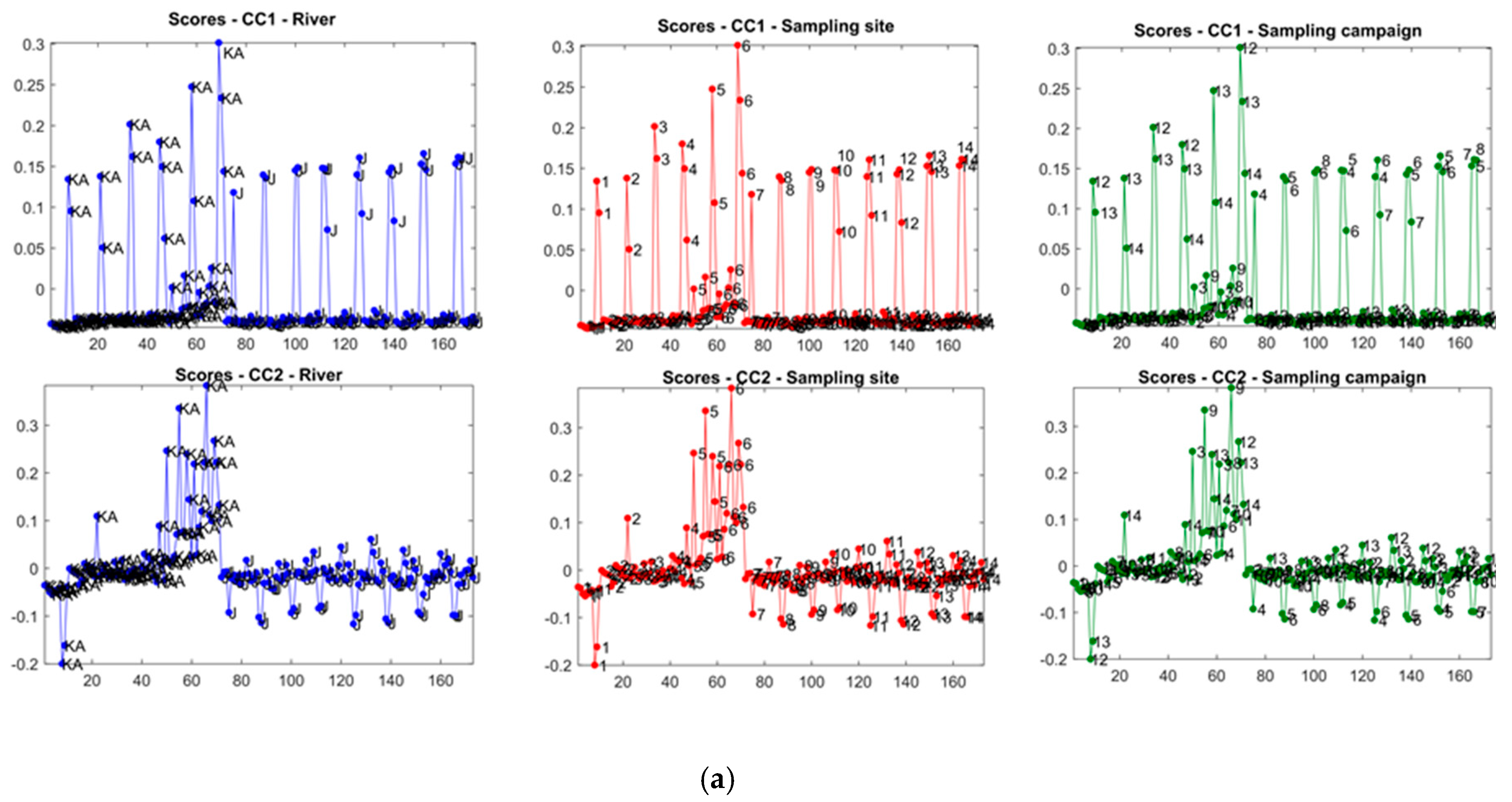
3.2.5. ComDim on 3D Fluorescence Data

ComDim was performed on fluorescence 3D EEMs, extracting 6 CCs. In the following, the first two CCs (CC1 and CC2) are considered (Figure 7), since they enclose relevant information related to specific spatiotemporal discriminations. The ComDim scores are presented in Figure 7a, where the same samples are labeled in three different ways to facilitate their interpretation: the river (KA: Kadisha-Abou Ali; J: El Jaouz), the sampling site (1 to 6 for the Kadisha-Abou Ali River and 7 to 14 for the El Jaouz River) and the sampling campaign covering the first 14 campaigns, ranging from July till February, at a frequency of 2 campaigns per month (labeled from 1 to 14). Saliences and loadings are presented in Figure 7b,c, respectively, showing the contribution of tentatively identified fluorophores in the highlighted discriminations.

According to CC1 scores (Figure 7a), all sites of the Kadisha-Abou Ali River are discriminated for the sampling campaigns 12, 13 and 14 corresponding to winter season (January and February). Moreover, all sites of the El Jaouz River are discriminated but for sampling campaigns from 4 (September) to 8 (October). These discriminations, which underline a seasonal variation, are influenced by two fluorophores highlighted by the saliences (Figure 7b) and the loadings (Figure 7c) of CC1. These signals were tentatively identified as aromatic proteins and fulvic acid like fluorophores (

Table 5. Spectral characteristics and tentative identification of ComDim loadings.

Common Component	Discriminated Samples	λex (max) nm	λem (max) nm	Tentative Identification	Reference
CC1	Rivers: KA and J Sites: all Campaigns: KA: 12/13/14 J: 4/5/6/7/8	200–210	300–375 (310)	Aromatic protein	[41,42]
		200–210	495–550 (540)	Fulvic acid like	[41]
CC2	River: K ASites: 5 and 6 Campaigns: all	315–388 (346)	380–480 (433)	Wastewater/nutrient enrichment tracer	[10,11,43]

, [10,11,41,42,43]). According to Xie et al. [42], the protein like fluorophore is frequently associated with anthropogenically derived organics in wastewater-impacted waters, whereas fulvic acids are a prevailing fraction of natural organic compounds [44]. These fluorophores have high seasonal dependency related to high flows in wet seasons and concentration effect in dry seasons [42]. In our case, the discrimination of El Jaouz River samples in dry season is probably related to concentration of natural organic compounds all along the river, whereas the Kadisha-Abou Ali River samples corresponding to the wet season may be influenced by increased wastewater discharges during this season. The last hypothesis may be supported by the spatial trend noticed on the Kadisha-Abou Ali scores, where the scores of campaigns 12, 13 and 14 increase when going down from the source towards the outlet, while the El Jaouz scores remain unchanged. Surprisingly, ComDim on EEMs shows the same trend as bivariate correlations (Figure 2) and PCA (Figure 3), along the course of the two studied rivers; the Kadisha-Abou Ali River is influenced by massive urban activities unlike the El Jaouz River, which is much less stressed by human activities.

CC2 scores highlight a very clear discrimination of sites KA5 and KA6 of the Kadisha-Abou Ali River. Based on the saliences (Figure 7b) and the loadings (Figure 7c) of CC2, the fluorophore implicated in this discrimination was tentatively identified as a characteristic of wastewater (Table 5). Once more, these sites appear as highly influenced by the anthropogenic discharges of surrounding agglomerations, mainly Tripoli. This result obtained on EEMs validates what was found by PCA analysis, which was based on physico-chemical and microbiological parameters. These similarities highlight the significant correlation between EEMs, organic physico-chemical and microbiological parameters, which validates the potential use of EEMs as a water quality indicator [32].

4. Conclusions

In this study, multivariate analyses, particularly PCA and ComDim, are successfully used to assess spatiotemporal variations in the surface water quality of two Lebanese rivers, the Kadisha-Abou Ali and El Jaouz. PCA and ComDim easily identify the spatial differences in surface water quality, the Kadisha-Abou Ali River being subjected to considerably greater anthropogenic stress than the El Jaouz River. In fact, sites KA5 and KA6 were particularly discriminated based on physico-chemical and microbiological indicators as well as on EEMs. Moreover, PCA and ComDim proved to be efficient in temporal studies, where score dispersion can be compared between sites in order to highlight any seasonal and/or anthropogenic variation. This multivariate approach combining physico-chemical, microbiological and fluorescence EEMs could be considered as a water quality fingerprint of the studied rivers, allowing the definition of a water mass reference, pillar for future monitoring. In fact, a water quality follow-up of Kadisha-Abou Ali River conducted seven years later shows a similar spatial distribution of samples KA1 to KA5 initially observed, with KA1 always considered as “water mass reference” and a slight improvement of KA5 water quality.

In conclusion, this methodology may be extrapolated to other fresh water ecosystems, in order to build their own water quality fingerprint, which will eventually lead to an easier and more reliable identification and monitoring of pollution sources. In fact, the natural variability intimately connected to environmental ecosystems constitutes one of the main challenges when interpreting water quality fingerprints. Pollution indicators should always be reassessed, for any new point or non-point source of pollution emerging over time.

References

1. United Nations. Sustainable Development Goals. Water Action Decade. Available online: https://www.un.org/sustainabledevelopment/water-action-decade/ (accessed on 3 June 2020).
2. Alberto, W.D.; Del Pilar, D.M.; Valeria, A.M.; Fabiana, P.S.; Cecilia, H.A.; Ángeles, B.M.d.l. Pattern Recognition Techniques for the Evaluation of Spatial and Temporal Variations in Water Quality. A Case Study. Water Res. 2001, 35, 2881–2894. [Google Scholar] [CrossRef]
3. Kowalkowski, T.; Zbytniewski, R.; Szpejna, J.; Buszewski, B. Application of chemometrics in river water classification. Water Res. 2006, 40, 744–752. [Google Scholar] [CrossRef] [PubMed]
4. Gazzaz, N.M.; Yusoff, M.K.; Ramli, M.F.; Aris, A.Z.; Juahir, H. Characterization of spatial patterns in river water quality using chemometric pattern recognition techniques. Mar. Pollut. Bull. 2012, 64, 688–698. [Google Scholar] [CrossRef] [PubMed]
5. Walker, D.; JakovljeviĆ, D.; Savic, D.; Radovanovic, M. Multi-criterion water quality analysis of the Danube River in Serbia: A visualisation approach. Water Res. 2015, 79, 158–172. [Google Scholar] [CrossRef]
6. Daou, C.; Salloum, M.; Legube, B.; Kassouf, A.; Ouaini, N. Characterization of spatial and temporal patterns in surface water quality: A case study of four major Lebanese rivers. Environ. Monit. Assess. 2018, 190, 485. [Google Scholar] [CrossRef]
7. Ates, N.; Kitis, M.; Yetis, U. Formation of chlorination by-products in waters with low SUVA—Correlations with SUVA and differential UV spectroscopy. Water Res. 2007, 41, 4139–4148. [Google Scholar] [CrossRef]
8. Barbosa, M.O.; Ribeiro, A.R.; Ratola, N.; Hain, E.; Homem, V.; Pereira, M.F.R.; Blaney, L.; Silva, A.M. Spatial and seasonal occurrence of micropollutants in four Portuguese rivers and a case study for fluorescence excitation-emission matrices. Sci. Total Environ. 2018, 644, 1128–1140. [Google Scholar] [CrossRef]
9. Powers, L.; Luek, J.L.; Schmitt-Kopplin, P.; Campbell, B.J.; Magen, C.; Cooper, L.; Gonsior, M. Seasonal changes in dissolved organic matter composition in Delaware Bay, USA in March and August 2014. Org. Geochem. 2018, 122, 87–97. [Google Scholar] [CrossRef]
10. Yan, C.; Liu, H.; Sheng, Y.; Huang, X.; Nie, M.; Huang, Q.; Baalousha, M. Fluorescence characterization of fractionated dissolved organic matter in the five tributaries of Poyang Lake, China. Sci. Total. Environ. 2018, 1311–1320. [Google Scholar] [CrossRef]
11. Murphy, K.R.; Hambly, A.; Singh, S.; Henderson, R.K.; Baker, A.; Stuetz, R.M.; Khan, S.J. Organic Matter Fluorescence in Municipal Water Recycling Schemes: Toward a Unified PARAFAC Model. Environ. Sci. Technol. 2011, 45, 2909–2916. [Google Scholar] [CrossRef]
12. Kannel, P.R.; Lee, S.; Kanel, S.; Khan, S.P. Chemometric application in classification and assessment of monitoring locations of an urban river system. Anal. Chim. Acta 2007, 582, 390–399. [Google Scholar] [CrossRef] [PubMed]
13. Barakat, A.; El Baghdadi, M.; Rais, J.; Aghezzaf, B.; Slassi, M. Assessment of spatial and seasonal water quality variation of Oum Er Rbia River (Morocco) using multivariate statistical techniques. Int. Soil Water Conserv. Res. 2016, 4, 284–292. [Google Scholar] [CrossRef]
14. Daou, C.; Nabbout, R.; Kassouf, A. Spatial and temporal assessment of surface water quality in the Arka River, Akkar, Lebanon. Environ. Monit. Assess. 2016, 188, 684. [Google Scholar] [CrossRef] [PubMed]
15. Wang, J.; Liu, G.; Liu, H.; Lam, P.K.; Lam, P.K. Multivariate statistical evaluation of dissolved trace elements and a water quality assessment in the middle reaches of Huaihe River, Anhui, China. Sci. Total Environ. 2017, 583, 421–431. [Google Scholar] [CrossRef] [PubMed]
16. Fernandes, A.; Fernandes, L.F.S.; Cortes, R.; Pacheco, F. The Role of Landscape Configuration, Season, and Distance from Contaminant Sources on the Degradation of Stream Water Quality in Urban Catchments. Water 2019, 11, 2025. [Google Scholar] [CrossRef] [Green Version]
17. Qannari, E.M.; Wakeling, I.; Courcoux, P.; MacFie, H.J. Defining the underlying sensory dimensions. Food Qual. Preference 2000, 11, 151–154. [Google Scholar] [CrossRef]
18. El Ghaziri, A.; Cariou, V.; Rutledge, D.N.; Qannari, E.M. Analysis of multiblock datasets using ComDim: Overview and extension to the analysis of (K + 1) datasets. J. Chemom. 2016, 30, 420–429. [Google Scholar] [CrossRef]
19. Karoui, R.; Dufour, E.; Schoonheydt, R.; De Baerdemaeker, J. Characterisation of soft cheese by front face fluorescence spectroscopy coupled with chemometric tools: Effect of the manufacturing process and sampling zone. Food Chem. 2007, 100, 632–642. [Google Scholar] [CrossRef]
20. Ministry of Environment (MOE). State of the Environment Report (SOER), Lebanon. MOE, UNDP and ECODIT, p. 47, 2010. Available online: http://www.undp.org.lb/communication/publications/downloads/SOER_en.pdf. (accessed on 3 September 2019).
21. Massoud, M.A.; El-Fadel, M.; Scrimshaw, M.; Lester, J. Factors influencing development of management strategies for the Abou Ali River in Lebanon. Sci. Total. Environ. 2006, 362, 15–30. [Google Scholar] [CrossRef]
22. Kabbara, N.; Benkhelil, J.; Awad, M.; Barale, V. Monitoring water quality in the coastal area of Tripoli (Lebanon) using high-resolution satellite data. ISPRS J. Photogramm. Remote Sens. 2008, 63, 488–495. [Google Scholar] [CrossRef]
23. Association Française de Normalisation (AFNOR) (French Association for Standardization). Qualité de l’eau—Recueil de Normes Françaises (Water Quality—Collection of French Standards); Association Française de Normalisation: Paris, France, 1994. [Google Scholar]
24. Cordella, C.B.; Bertrand, D. SAISIR: A new general chemometric toolbox. TrAC Trends Anal. Chem. 2014, 54, 75–82. [Google Scholar] [CrossRef]
25. Bouroche, J.M.; Saporta, G. L’analyse des données. Collection Que sais-je? In Data Analysis. Collection What Do I Know; Presses Universitaires de France: Paris, France, 1992. [Google Scholar]
26. Singh, K.P.; Malik, A.; Sinha, S. Water Quality Assessment and Apportionment of Pollution Sources of Gomti River (India) Using Multivariate Statistical Techniques—A Case Study. Anal. Chim. Acta 2005, 538, 355–374. [Google Scholar] [CrossRef]
27. Bouveresse, D.J.-R.; Pinto, R.C.; Schmidtke, L.; Locquet, N.; Rutledge, D. Identification of significant factors by an extension of ANOVA–PCA based on multi-block analysis. Chemom. Intell. Lab. Syst. 2011, 106, 173–182. [Google Scholar] [CrossRef]
28. Rosa, L.N.; De Figueiredo, L.C.; Bonafé, E.G.; Coqueiro, A.; Visentainer, J.V.; Março, P.H.; Rutledge, D.N.; Valderrama, P. Multi-block data analysis using ComDim for the evaluation of complex samples: Characterization of edible oils. Anal. Chim. Acta 2017, 961, 42–48. [Google Scholar] [CrossRef]
29. Bouhlel, J.; Bouveresse, D.J.-R.; Abouelkaram, S.; Baéza, E.; Jondreville, C.; Travel, A.; Ratel, J.; Engel, E.; Rutledge, D.N. Comparison of common components analysis with principal components analysis and independent components analysis: Application to SPME-GC-MS volatolomic signatures. Talanta 2018, 178, 854–863. [Google Scholar] [CrossRef]
30. Bouza-Deaño, R.; Rodriguez, M.T.; Fernández-Espinosa, A. Trend study and assessment of surface water quality in the Ebro River (Spain). J. Hydrol. 2008, 361, 227–239. [Google Scholar] [CrossRef]
31. Varol, M. Spatio-temporal changes in surface water quality and sediment phosphorus content of a large reservoir in Turkey. Environ. Pollut. 2020, 259, 113860. [Google Scholar] [CrossRef]
32. Tang, J.; Li, X.; Cao, C.; Lin, M.; Qiu, Q.; Xu, Y.; Ren, Y. Compositional variety of dissolved organic matter and its correlation with water quality in peri-urban and urban river watersheds. Ecol. Indic. 2019, 104, 459–469. [Google Scholar] [CrossRef]
33. Razmkhah, H.; Abrishamchi, A.; Torkian, A. Evaluation of spatial and temporal variation in water quality by pattern recognition techniques: A case study on Jajrood River (Tehran, Iran). J. Environ. Manag. 2010, 91, 852–860. [Google Scholar] [CrossRef]
34. Vega, M.; Pardo, R.; Barrado, E.; Deban, L. Assessment of seasonal and polluting effects on the quality of river water by exploratory data analysis. Water Res. 1998, 32, 3581–3592. [Google Scholar] [CrossRef]
35. El Najjar, P.; Kassouf, A.; Probst, A.; Probst, A.; Ouaini, N.; Daou, C.; El Azzi, D. High-frequency monitoring of surface water quality at the outlet of the Ibrahim River (Lebanon): A multivariate assessment. Ecol. Indic. 2019, 104, 13–23. [Google Scholar] [CrossRef] [Green Version]
36. Ruždjak, A.M.; Ruždjak, D. Evaluation of river water quality variations using multivariate statistical techniques. Environ. Monit. Assess. 2015, 187, 1–14. [Google Scholar] [CrossRef]
37. Zheng, L.-Y.; Yu, H.-B.; Wang, Q.-S. Assessment of temporal and spatial variations in surface water quality using multivariate statistical techniques: A case study of Nenjiang River basin, China. J. Central South Univ. 2015, 22, 3770–3780. [Google Scholar] [CrossRef]
38. Ustaoğlu, F.; Tepe, Y.; Taş, B. Assessment of stream quality and health risk in a subtropical Turkey river system: A combined approach using statistical analysis and water quality index. Ecol. Indic. 2020, 113, 105815. [Google Scholar] [CrossRef]
39. Karakaya, N.; Evrendilek, F. Water quality time series for Big Melen stream (Turkey): Its decomposition analysis and comparison to upstream. Environ. Monit. Assess. 2009, 165, 125–136. [Google Scholar] [CrossRef] [PubMed]
40. David, A.; Tournoud, M.-G.; Perrin, J.-L.; Rosain, D.; Rodier, C.; Salles, C.; Bancon-Montigny, C.; Picot, B. Spatial and temporal trends in water quality in a Mediterranean temporary river impacted by sewage effluents. Environ. Monit. Assess. 2012, 185, 2517–2534. [Google Scholar] [CrossRef]
41. Chen, W.; Westerhoff, P.; Leenheer, J.A.; Booksh, K. Fluorescence Excitation−Emission Matrix Regional Integration to Quantify Spectra for Dissolved Organic Matter. Environ. Sci. Technol. 2003, 37, 5701–5710. [Google Scholar] [CrossRef]
42. Xie, M.-W.; Chen, M.; Wang, W.-X. Spatial and temporal variations of bulk and colloidal dissolved organic matter in a large anthropogenically perturbed estuary. Environ. Pollut. 2018, 243, 1528–1538. [Google Scholar] [CrossRef]
43. Galinha, C.F.; Carvalho, G.; Portugal, C.; Guglielmi, G.; Reis, M.A.M.; Crespo, J.G. Two-dimensional fluorescence as a fingerprinting tool for monitoring wastewater treatment systems. J. Chem. Technol. Biotechnol. 2011, 86, 985–992. [Google Scholar] [CrossRef]
44. Klimenko, N.A.; Samsoni-Todorova, E.A.; Savchina, L.A.; Lavrenchuk, I.N.; Zasyad’Ko, T.N. Seasonal variations of characteristics of organic matter in the Dnieper River water. J. Water Chem. Technol. 2012, 34, 154–161. [Google Scholar] [CrossRef]
Figure 1. Map of the Kadisha-Abou Ali and El Jaouz rivers. Red dots refer to the monitoring sites (KA1 to KA6 for Kadisha-Abou Ali River and J7 to J14 for El Jaouz River).
Water 12 01673 g001
Figure 2. Number of couples of correlated variables with Pearson coefficient >0.5 for each station of the Kadisha Abou Ali (a) and El Jaouz (b) rivers.
Water 12 01673 g002
Figure 3. Scatter plot of scores corresponding to: (a) the first two principal components; (b) the first and third components, for the two river sites during the entire study period.
Water 12 01673 g003
Figure 4. Scatter plot of scores during the study period, corresponding to the first two principal components for all stations excluding KA5 and KA6.
Water 12 01673 g004
Figure 5. Scatter plot of the scores for sites KA1 and KA2 corresponding to 26 sampling campaigns labeled by season: (1) summer, (2) autumn, (3) winter and (4) spring.
Water 12 01673 g005
Figure 6. Scatter plot of scores during two sampling campaigns (2003 and 2010), corresponding to the first two principal components, for stations KA1 to KA5 of the Kadisha-Abou Ali River.
Water 12 01673 g006
Figure 7. ComDim results on CC1 and CC2: (a) scores, (b) saliences and (c) loadings.
Water 12 01673 g007aWater 12 01673 g007b