Article

B-Spline Method of Lines for Simulation of Contaminant Transport in Groundwater

Department of Civil Engineering, Pamukkale University, Denizli 20160, Turkey
*
Author to whom correspondence should be addressed.
Water 2020, 12(6), 1607; https://doi.org/10.3390/w12061607
Submission received: 1 April 2020 / Revised: 29 May 2020 / Accepted: 31 May 2020 / Published: 4 June 2020

Abstract

:
In this study, we propose a new numerical method, which can be effectively applied to the advection-dispersion equation, based on B-spline functions and method of lines approach. In the proposed approach, spatial derivatives are calculated using quintic B-spline functions. Thanks to the method of lines approach, the partial differential equation governing the contaminant transport in groundwater is converted into time-dependent ordinary differential equations. After this transformation, the time-integration of this system is realized by using an adaptive Runge–Kutta formula. In order to test the accuracy of the proposed method, four numerical examples were solved and the obtained results compared with various analytical and numerical solutions given in the literature. It is proven that the proposed method is faster and more reliable than other methods referenced herein and is a good alternative for simulation of contaminant transport problems as a result of these comparisons.

1. Introduction

Groundwater is one of the most important resources in the world. This resource is used as clean water in many different fields such as domestic, industrial and agricultural. Especially in rural areas, most of the people’s need for clean water is met by groundwater. The need for clean water is increasing with the increase in the world population and the development of industrial and agricultural technologies. Therefore, both the quantity and the quality of groundwater are very important, because contaminated groundwater loses its intended use. In such cases, remediation works should be carried out for contaminated groundwater. In these studies, modeling of contaminant transport in the relevant region is very important as it will provide an analysis of the current situation and provide information about the future status of the current pollution [1].
Groundwater contaminant transport modeling is carried out by solving the partial differential equation which represents the physical processes occur in nature, under certain boundary and initial conditions using analytical or numerical methods. Analytical models produce continuous results in the solution space, but these models are available only for simplified cases with simple geometry and constant parameters. However, the geometry of contamination problems encountered in the real world is complex, and its parameters vary depending on location and time. For this reason, it is mandatory to use numerical models in real-world applications. Although numerical models produce discrete solutions at the nodes, they are preferred because they can provide solutions when the geometry is complex and the parameters are variable [2].
In last two decades many different numerical models have been developed for the solution of contaminant transport problem. These models are based on different approaches such as finite difference method [3,4,5,6], finite element method [7], finite volume method [8], boundary element method [9], collocation method [10], meshfree method [11,12], operator splitting method [13], compact finite difference method [14,15], lattice Boltzmann method [16,17] and differential quadrature method [18].
Recently, methods based on B-spline functions are getting a lot of attention from researchers due to their simple application, low computational efforts and cost in the solution of transport problems. For example, Irk et al. [19] proposed extended cubic B-spline collocation method for space and Crank–Nicolson for time integration in solution of advection–diffusion equations. They compared obtained results with cubic B-spline collocation method. Dhawan et al. [20] developed a finite element method that uses linear and quadratic B-spline functions. Korkmaz and Dag [21] proposed differential quadrature methods based on quartic and quintic B-spline functions for the approximation of space derivatives. By using approximated derivatives, they transformed partial differential equation into ordinary differential equations system. Then applied fourth order Runge–Kutta and sixth order Runge–Kutta–Butcher methods for the time integration. Nazir et al. [22] proposed cubic trigonometric B-spline functions with collocation method for the solution of wide range of one-dimensional advection–diffusion problems. In their work, weighted finite difference approach was used for time integration. Mohammadi [23] presented exponential B-spline collocation method for space and Crank–Nicolson formulation for time integration for the solution of convection-diffusion equation. Mittal and Tripathi [24] developed modified bi-cubic B-spline finite elements method for the solution two-dimensional convection–diffusion equation. Rohila and Mittal [25] proposed an alternating implicit direction method based on bi-cubic B-spline functions for the solution of the two-dimensional advection–diffusion equation. Shukla and Tamsir [26] presented an exponential modified cubic B-spline differential quadrature method to approximate the solution of two- and three-dimensional convection–diffusion equations. It is clear that different types of third order B-spline functions widely used for the solution of transport problems, but more work has to be done to develop more efficient numerical schemes, especially for the multi-dimensional problems.
The main objective of this study is to propose a method of lines-based approach for contaminant transport problems. In the proposed approach, the partial differential equation governing the contaminant transport in groundwater converted into time-dependent ordinary differential equations. After this transformation, the integration of these equations carried out by using the fifth-order adaptive Runge–Kutta formula of Dormand and Prince [27]. This is a novel, simple and effective numerical method for modeling of the two-dimensional contaminant transport in groundwater. The performance of the proposed approach is evaluated by solving four numerical applications from the literature. The results showed that the proposed approach not only achieved the accurate solution of the contaminant transport problem but also significantly reduced the CPU time.

2. Governing Equations

The partial differential equation describes the transport of a single chemical constituent in saturated porous media in two-dimensions, considering the advection–dispersion process is given by [2].
C t = x ( D x x C x ) + x ( D x y C y ) + y ( D y x C x ) + y ( D y y C y ) x ( V x C ) y ( V y C )
where V x and V y are seepage velocities in x and y directions ( LT 1 ); D x x , D x y , D y x and D y y are the elements of the dispersion coefficient tensor ( L 2 T 1 ); C is dissolved concentration ( MT 3 ); x and y are cartesian coordinates ( L ); t is time ( T ).
The elements of the dispersion coefficient tensor D x x , D x y , D y x and D y y can be calculated by using seepage velocities and longitudinal ( α L ) and transverse ( α T ) dispersivities from relations given in Equation (2) [28].
D x x = α L V x 2 + α T V y 2 V x 2 + V y 2 + D * ;   D x y = D y x = V x V y ( α L α T ) V x 2 + V y 2 ;   D y y = α L V y 2 + α T V x 2 V x 2 + V y 2 + D *
where D * is the effective molecular diffusion coefficient. The molecular diffusion coefficient is extremely small compared to the mechanical dispersion coefficient. For this reason, it can be neglected in calculations.

3. B-Spline Method of Lines

In the proposed method, MOL is used with the QBS functions for numerical discretization of the Equation (1). Firstly, space derivatives are approximated with the help of the QBS functions. Then the approximated space derivatives are written in Equation (1). Thus, the problem transforms to time-dependent system of ordinary differential equations. This system is solved with the help of DOPRI5. The formulation of this solution is presented in the following sections.

3.1. Spatial Discretization

Let the two-dimensional solution domain partitioned into a mesh of uniform lengths Δ x = x i + 1 x i and Δ y = y j + 1 y j , by the nodes ( x i , y j ) where i = 0 , 1 , , N and j = 0 , 1 , , M . Our goal is to construct QBS functions for every vector in both directions. Then, space derivatives at the nodes can be calculated easily without needing complicated formulations. It is clear that solution domain consists of M + 1 row vectors and N + 1 column vectors. Therefore, ( M + 1 ) × ( N + 1 ) times numerical approximations for contaminant concentrations are established with QBS functions for both x - and y -directions.
The concentration values C ( x , y , t ) can be approximated by C ˜ ( x , y , t ) with QBS functions. The mathematical formulation of QBS functions is given below considering the row and column vectors in x - and y -directions.
C ( x , y j , t ) C ˜ ( x , y j , t ) = i = 2 N + 2 δ j , i ( t ) B i ( x ) ,   f o r   j = 0 , 1 , , M
C ( x i , y , t ) C ˜ ( x i , y , t ) = j = 2 M + 2 γ j , i ( t ) Q j ( y ) ,   f o r   i = 0 , 1 , , N
where δ j , i ( t ) and γ j , i ( t ) are time-dependent parameter matrices that are needed to be calculated by using initial and boundary conditions. B i ( x ) and Q j ( y ) are the QBS basis functions for x - and y -directions given in Equations (5) and (6), respectively [29].
B i ( x ) = 1 x 5 { ( x x i 3 ) 5 x [ x i 3 , x i 2 ) ( x x i 2 ) 5 6 ( x x i 2 ) 5 x [ x i 2 , x i 1 ) ( x x i 3 ) 5 6 ( x x i 2 ) 5 + 15 ( x x i 1 ) 5 x [ x i 1 , x i ) ( x i + 3 x ) 5 6 ( x i + 2 x ) 5 + 15 ( x i + 1 x ) 5 x [ x i , x i + 1 ) ( x i + 3 x ) 5 6 ( x i + 2 x ) 5 x [ x i + 1 , x i + 2 ) ( x i + 3 x ) 5 x [ x i + 2 , x i + 3 ) 0 otherwise
Q j ( y ) = 1 y 5 { ( y y j 3 ) 5 y [ y j 3 , y j 2 ) ( y y j 3 ) 5 6 ( y y j 2 ) 5 y [ y j 2 , y j 1 ) ( y y j 3 ) 5 6 ( y y j 2 ) 5 + 15 ( y y j 1 ) 5 y [ y j 1 , y j ) ( y j + 3 y ) 5 6 ( y j + 2 y ) 5 + 15 ( y j + 1 y ) 5 y [ y j , y j + 1 ) ( y j + 3 y ) 5 6 ( y j + 2 y ) 5 y [ y j + 1 , y j + 2 ) ( y j + 3 y ) 5 y [ y j + 2 , y j + 3 ) 0 otherwise
The values of QBS basis functions and its first and second order derivatives at nodal points are given in Table 1 and Table 2. Obviously, third and fourth order derivatives can be calculated as well but as it is clear from Equation (1) that only first and second order derivatives are needed.
Approximate concentration values and its first and second order derivatives at the nodes in both directions can be calculated in terms of δ j , i ( t ) and γ j , i ( t ) by using approximate functions in Equations (3) and (4) with the values of QBS functions given in Table 1 and Table 2. The steps required to find the δ j , i ( t ) and γ j , i ( t ) values are presented in detail in Appendix A.

3.2. Temporal Discretization

MOL is a powerful approach in which partial differential equation transforms to ordinary differential equation system. The main advantage of this approach is that in the integration of ordinary differential equation system well-established, robust, thoroughly tested integrators can be used [30]. When the spatial derivatives of the contaminant transport equation given in Equation (1) are discretized by QBS functions, the time-dependent ordinary differential equation system given below is obtained.
d C d t = ( t , C )
where indicates a spatial differential operator. A fifth-order adaptive Runge–Kutta formula, known as DOPRI5 [27], is used for the time integration of the Equation (7) which consists of ( M + 1 ) × ( N + 1 ) ordinary differential equations.
The DOPRI5 is an adaptive integration method used in the solution of ordinary differential equations and is a member of the Runge–Kutta family [27]. It has seven stages, but it uses only six function evaluations per step because it has the FSAL (First Same as Last) property: the last stage is evaluated at the same point as the first stage of the next step. The coefficients in the DOPRI5 are chosen to minimize the error of the fifth order solution. This is the main difference with the Fehlberg method [31], which was constructed so that the fourth-order solution has a small error. For this reason, the DOPRI5 method is more suitable when the higher-order solution is used to continue the integration, a practice known as local extrapolation [32]. Such adaptive time-integration methods always keep the truncation errors below a certain value for each step and prevent the errors from growing uncontrollably. In other words, the numerical errors are prevented from overgrowth, and the stability of the numerical method is maintained. The numerical concentration values for successive time steps are calculated with the DOPRI5 scheme as follows:
k 1 = ( t p , C p )
k ν = ( t p + ω ν t p , C p + t p ξ = 1 ν 1 ϕ ν , ξ k ξ ) ,   ν = 2 , 3 , , 7
C p + 1 = C p + t p ν = 1 7 ψ ν k ν
where p and ν represent time and stage indexes, k ν is the approximated slope matrix calculated at each stage, t p is the dynamically determined time step at time t p , the coefficients ω ν ,   ϕ ν , ξ ,   ψ ν are elements of Butcher array which is given in Table 3 [33].
The local truncation error for the DOPRI5 scheme is obtained approximately by the formula given in Equation (11). The infinity norm of this error matrix is compared to a user-defined maximum allowable error tolerance. If the e p + 1 e t o l condition is satisfied, the time step is calculated according to the formulation given in Equation (12). Otherwise, t p + 1 is iteratively updated using Equation (12) until e p + 1 e t o l condition is satisfied. In this study, the t p + 1 / t p ratio was limited to [ 0.1 , 10 ] and e t o l = 1 × 10 6 .
e p + 1 = t p ν = 1 7 ( ψ ν ψ ^ ν ) k ν
t p + 1 = 0.9 t p ( e t o l e p + 1 ) 1 5 ,   e p + 1 e t o l

4. Numerical Applications

In this section, the success of the proposed method (QBS-DOPRI5) will be tested on four different problems, which are widely used in the literature. All problems were solved with QBS-DOPRI5 and their results were compared with analytical or numerical solutions given in the literature. In the following section, detailed information about this comparison will be presented. All simulations are performed on a computer with an i5-4460 processor with 3.20 GHz speed and 8 GB RAM.

4.1. Example 1

Consider Equation (1) with constant parameters such as V x = V y = 0.8   m / s and D x x = D y y = 0.01   m 2 / s , D x y = D y x = 0   m 2 / s and the solution domain of 0 < x , y < 2 . Analytical solution of this problem was given by Kalita et al. [34].
C ( x , y , t ) = 1 1 + 4 t e x p ( ( x x ^ V x t ) 2 D x x ( 1 + 4 t ) ( y y ^ V y t ) 2 D y y ( 1 + 4 t ) )
In this problem, a Gaussian pulse is considered as an initial condition with the peak value of unity. Location of the peak value is indicated by ( x ^ , y ^ ) , which is taken as ( 0.5 , 0.5 ) in the experiments. The initial and boundary conditions can be taken from the analytical solution. To compare our results with the other proposed numerical methods in the literature, the same simulation parameters such as flow velocities, dispersion coefficients and grid sizes are used. Example 1 has been studied by many researchers to test their proposed methods. Comparisons were made in terms of average and maximum absolute errors. Average absolute error values at the time t = 1   s over the domain [ 1 , 2 ] × [ 1 , 2 ] with V x = V y = 0.8   m / s and D x x = D y y = 0.005   m 2 / s are presented in Table 4. QBS-DOPRI5 is produced better average absolute error values than the other methods given in Table 4.
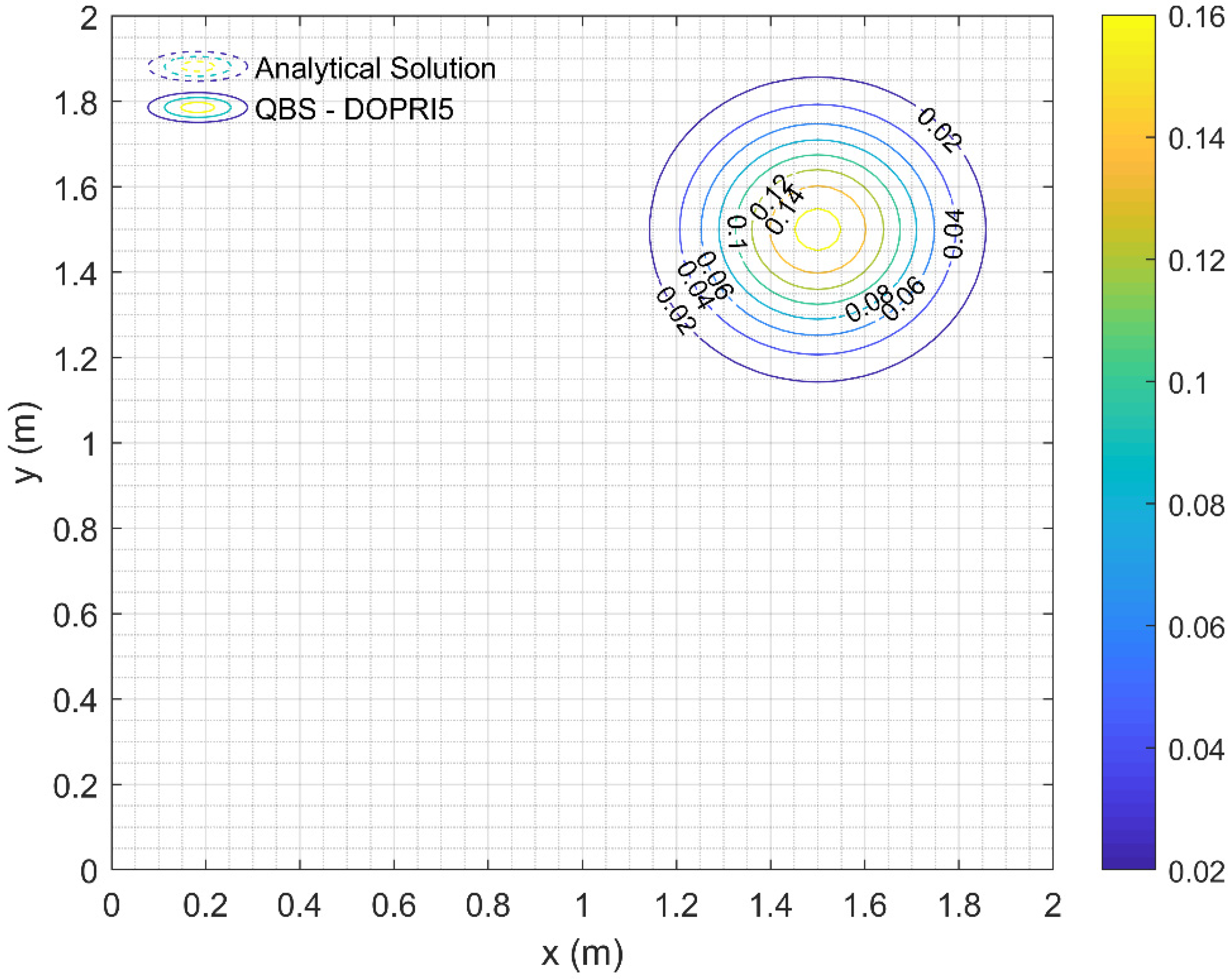
The parameters used in Table 5 are V x = V y = 0.8   m / s , D x x = D y y = 0.01   m 2 / s , D x x = D y y = 0.001   m 2 / s and x = y = 0.025   m . In Table 5, both average absolute error and maximum error values are presented and compared with the results of the other available numerical methods in the literature. It is clear that QBS-DOPRI5 produces error values similar to or lower than other methods. Moreover, the results obtained with QBS-DOPRI5 at time t = 1.25   s for x = y = 0.025   m , V x = V y = 0.8   m / s , D x x = D y y = 0.01   m 2 / s are plotted in Figure 1 in which Gaussian shape of the concentration can be seen clearly. The contour lines of these results are plotted in Figure 2.
QBS-DOPRI5 consists of high-order schemes both in time and space. Therefore, both DOPRI5 and QBS schemes contribute to the quality of the solution. It is obvious that if Euler scheme was preferred instead of DOPRI5 scheme for time integration, the results would not be accurate enough. In order to prove this situation, this example is solved with QBS-Euler and the results are compared with QBS-DOPRI5.
It should be noted that the smallest time step chosen in the methods presented in Table 5 (except QBS-DOPRI5) is t = 0.00625   s . In the QBS-Euler method, the time step is reduced by 50 times and taken into consideration as t = 0.000125   s . The average absolute error and maximum absolute error values obtained with the QBS-Euler method for D x x = D y y = 0.01   m 2 / s are 2.435 × 10 5 and 5.572 × 10 4 , respectively. It is clear that the error values given in Table 5 for QBS-DOPRI5 are considerably smaller than the error values obtained with QBS-Euler. CPU times required for QBS-Euler and QBS-DOPRI5 are obtained as 335.57 s and 17.48 s, respectively. As a result of this analysis, it is necessary to use high-order schemes together in space and time, both in terms of the quality of the solutions and the reduction of the CPU time.

4.2. Example 2

In this example, migration of chloride ion in landfill leachate through a narrow, relatively thin, valley-fill aquifer is considered in which the simulation is governed by Equation (1). This example is taken from the work of Wexler [38], the sample problem 6. Boundary conditions of the problem are as follows:
C ( x , y , t ) = { C ^ , x = x 0   and   y ^ 1 y y ^ 2 0 , x = x 0   and   y y ^ 1   or   y y ^ 2
and
C / x = 0 , x = x N C / y = 0 , y = y 0   or   y = y M
where, y M = 1200   m is the aquifer width, y ^ 1 = 300   m , y ^ 2 = 800   m , x N = 1500   m is the aquifer length, C ^ = 1   kg / m 2 , flow velocities are V x = 3 × 10 6   m / s , V y = 0 and dispersion coefficients are D x x = 2 × 10 4   m 2 / s , D y y = 6 × 10 5   m 2 / s . According to the assumptions of Wexler [38], D x y and D y x dispersion coefficients are taken as zero. Under these conditions, analytical solution of the problem given by Wexler [38]
C ( x , y , t ) = C ^ n = 0 L n P n c o s ( η y ) { e x p [ x ( V x β ) 2 D x x ] e r f c [ x β t 2 D x x t ] + e x p [ x ( V x + β ) 2 D x x ] e r f c [ x + β t 2 D x x t ] }
in which
L n = { 0.5 , n = 0 1 , n > 0
P n = { ( y ^ 2 y ^ 1 ) / y M , n = 0 [ s i n ( η y ^ 2 ) s i n ( η y ^ 1 ) ] / ( n π ) , n > 0
η = n π / y M ,   n = 0 , 1 , 2 , 3 ,
β = V x 2 + 4 η 2 D x x D y y
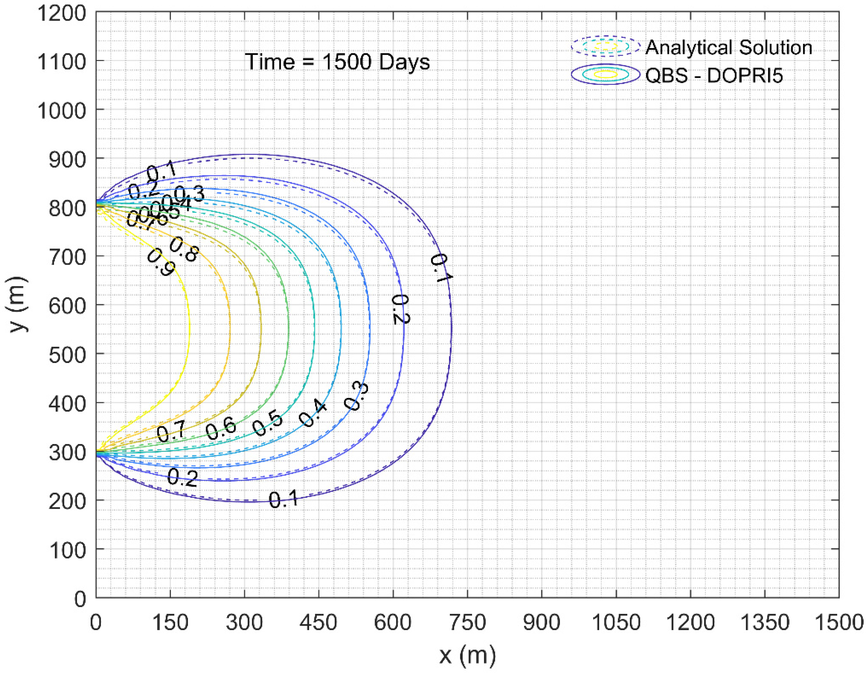
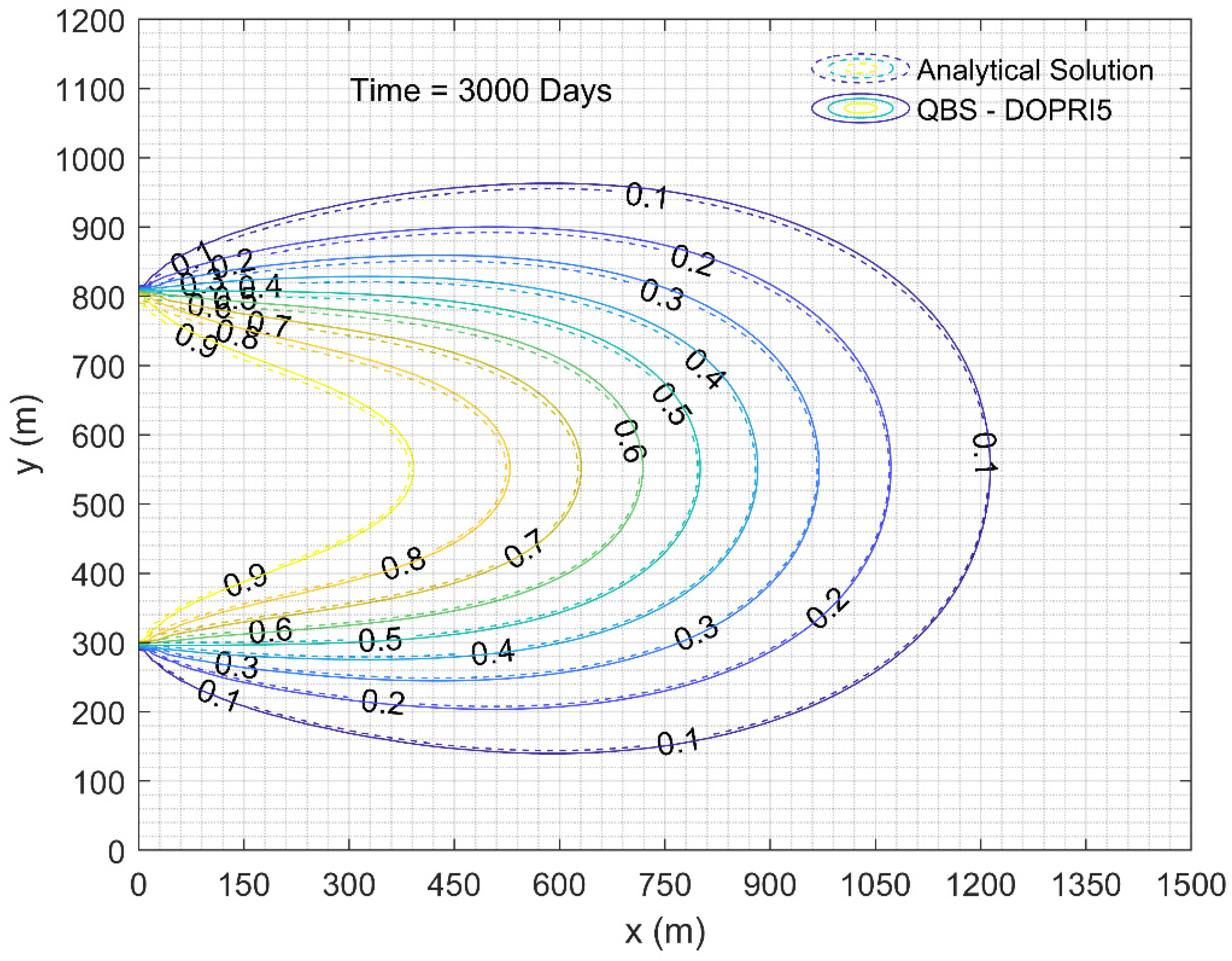
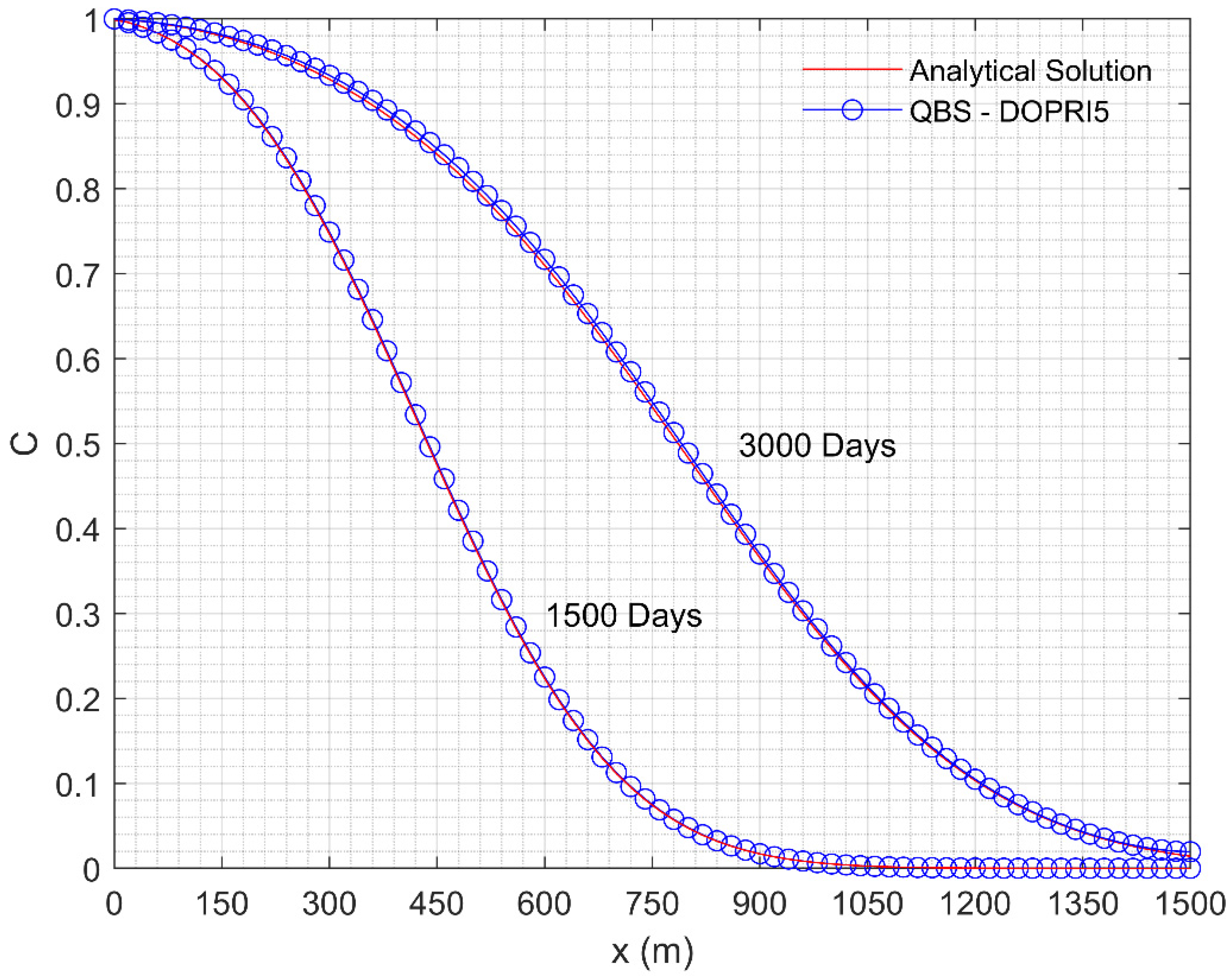
Simulations are carried out for different times, i.e., t = 1500 days, t = 3000 days. Contour lines of the approximated concentration results for different simulation times are plotted in Figure 3 and Figure 4 together with the analytical solution, showing very good agreement. Moreover, central concentration profiles are compared and plotted in Figure 5. An excellent agreement was observed.

4.3. Example 3

In this example, an unsymmetrical continuous solute line source at the left boundary ( x = x 0 ) is considered. The concentrations of the solute source at the boundary are calculated by the following formulation [9,11].
C ( x 0 , y , t ) = C ^ ( ( y y ^ ) 2 3140 )
where, C ^ is the peak value of concentration at the line source and assumed to be unity. This way obtained concentration values can be considered as relative concentrations. y ^ = 125   m is the location of the peak concentration value at solute line source. The other boundary conditions are assumed to be no flux and mathematical representation of them are as follows:
C / x = 0 , x = x N C / y = 0 , y = y 0   or   y = y M
where y M = 300   m and x N = 600   m are the width and length of the aquifer field, respectively. Two-dimensional velocity field is considered. The simulations are conducted by taking velocities as V x = 1.1784   m / d and V y = 0.3157   m / d . Dispersion coefficients are calculated from Equation (2) by taking longitudinal dispersivity, α L = 6.248 m, and transverse dispersivity, α T = 0.393 m. As can be seen from the parameters, the aquifer is homogeneous and anisotropic. For this reason, the x ( D x y C y ) and y ( D y x C x ) terms in Equation (1) must be included in the solution. However, in the works of Eldho and Rao [9] and Boddula and Eldho [11], it is seen that these terms are not included in the solution. Two different scenarios are examined for this example. In the first scenario (Scenario A), these terms are neglected in order to compare the solutions under the same conditions. In the second scenario (Scenario B), these terms are taken into account in order to see the real behavior of the problem.
Since there is no available analytical solution for this problem, FDM-DOPRI5 was developed and used to obtain a reference solution by taking space grid sizes considerably small such as h = x = y = 0.5 m for scenario A and h = x = y = 0.25 m for scenario B. These grid sizes mean 1201 × 601 nodes for scenario A and 2401 × 1201 nodes for scenario B are presented in the solution domain. The solutions obtained with these many nodes can be considered as almost exact solutions.
The obtained results with the QBS-DOPRI5 considering Scenario A are compared with the other solutions taken from the literature in Table 6 for different grid sizes. QBS-DOPRI5 produced very good results even when the grid size h = 25 m, which means 25 × 13 nodes in the solution domain. For h = 5 m, meaning 121 × 61 nodes, the obtained concentration values with QBS-DOPRI5 are almost identical with reference solution. Contour lines of the approximated solution obtained by QBS-DOPRI5 and reference solution are plotted in Figure 6. As clearly seen from Figure 6, the contour lines of the solutions are identical.
Table 7 was created to show that the proposed method achieved the same accuracy in a shorter time than standard numerical methods. As can be seen from Table 7, solutions for QBS-DOPRI5 and FDM-DOPRI5 for different h values were obtained, and their concentration values at different locations were given. CPU times spent for these solutions are also presented in the same table. When Table 7 is examined carefully, the solutions obtained for QBS-DOPRI5 with h = 25 / 4   m and FDM-DOPRI5 with h = 25 / 32   m appear to be the same as the reference solution. Comparing the CPU times (19.57 s and 1302.46 s) obtained in this case, it is obvious that the QBS-DOPRI5 method is 66.55 times faster than the FDM-DOPRI5 method.
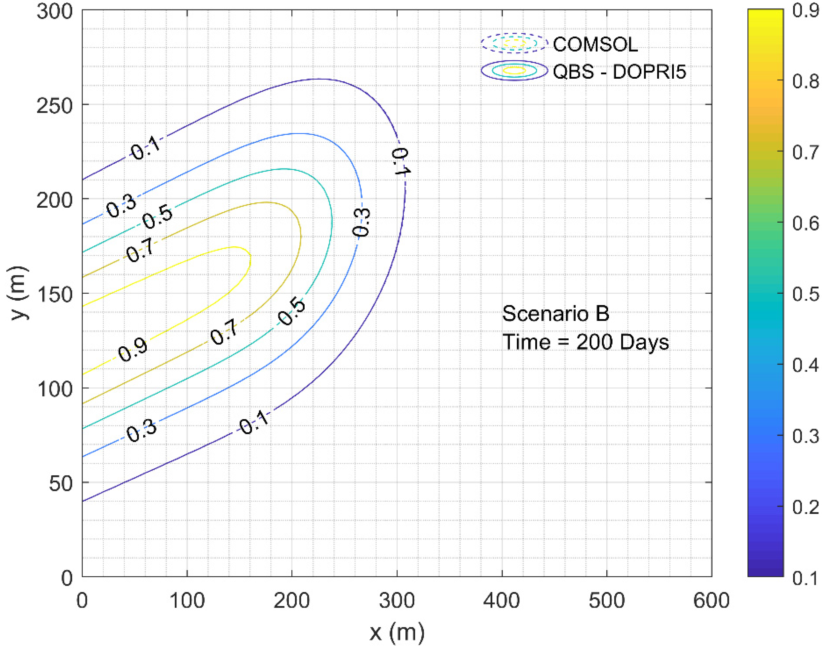
When the same problem is solved considering scenario B, the results are presented in Table 8. As can be seen from Table 8, QBS-DOPRI5 with h = 25 / 4   m and FDM-DOPRI5 with h = 25 / 64   m reach the same accuracy as the reference solution. Comparing the CPU times spent under these conditions, QBS-DOPRI5 was found to be 1061.82 times faster than FDM-DOPRI5. Moreover, this example is solved with COMSOL Multiphysics, the well-known FEM commercial code, under scenario B. This solution was obtained by activating the adaptive mesh refinement property in the COMSOL Multiphysics program and using 30763 triangular elements. It should be noted that QBS-DOPRI5 and COMSOL Multiphysics results are exactly the same. These results are illustrated in Figure 7. Also, COMSOL Multiphysics output results used to plot Figure 7 are presented in Table S1 file in Supplementary Materials.

4.4. Example 4

In reality, the aquifers are complex and can vary significantly in terms of physical parameters, such as permeability and diffusivity. For this reason, an example that is given in the work of Perko [17] is studied. In this example, anisotropic dispersion with spatially varying velocity field is considered for testing the proposed method’s robustness. The problem is invariant in the z - direction. Hence, it can be considered as a 2D problem. The velocity components in x - and y - directions are as follows:
V x = 2 y ( 1 x 2 )
V y = 2 x ( 1 y 2 )
A rectangular flow domain is considered with the dimensions 1 x 1 and 0 y 1 . Dirichlet boundary condition is considered along the left bottom boundary ( 1 x 0 , y = 0 ). The concentration profile at the Dirichlet boundary varies from 0 to 1 as a sharp pulse-like shape. Open boundary condition is defined along the right bottom boundary ( 0 x 1 , y = 0 ). The Dirichlet boundary concentration profile is defined as
C ( x , t ) = tanh   ( ϒ ( 0.6 + x ) ) tan h ( ϒ ( 0.4 + x ) ) 2
where the parameter ϒ determines the sharpness of the concentration profile. The value of ϒ is taken as 100, which results in a sharp profile. Neumann boundary condition with zero flux is defined at the left, right and upper boundaries.
Since this example also does not have an analytical solution, a reference solution is needed to compare QBS-DOPRI5 results. For this purpose, a reference solution is obtained by activating the adaptive mesh refinement property within the COMSOL Multiphysics software. In this example, two different scenarios are created by changing the ratio of the longitudinal dispersivity to transverse dispersivity coefficients. In the first scenario (scenario A), a typical ratio of 10 is considered by taking α L = 0.1 m and α T = 0.01 m. In the second scenario (scenario B), this ratio is taken as 1000 in order to test the real potential of the proposed method. In this scenario, dispersivities are selected as α L = 1   m and α T = 0.001 m. COMSOL Multiphysics models contain 25,806 and 106,268 triangular elements in the solution domain for Scenarios A and B, respectively.
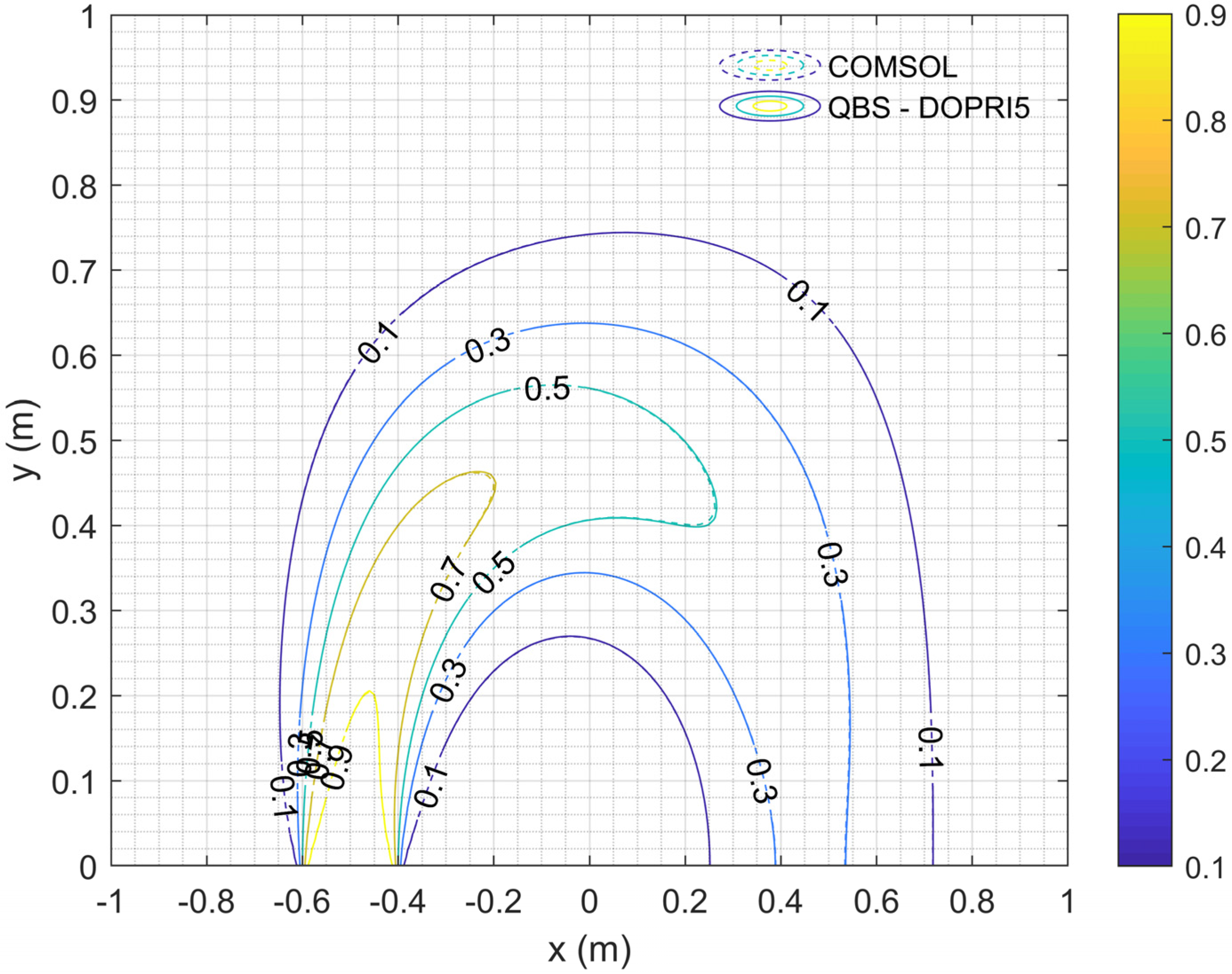
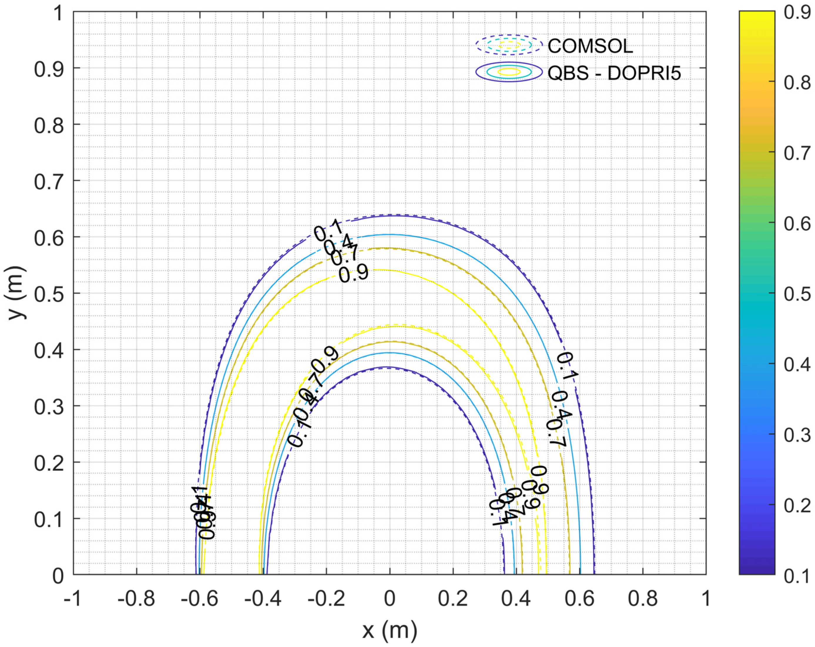
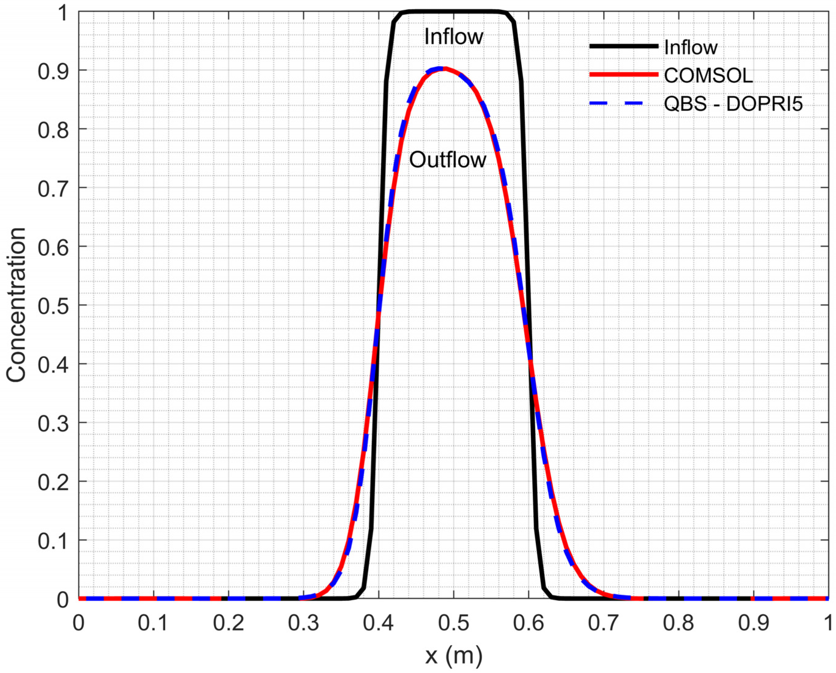
The contour plot of the solutions obtained with QBS-DOPRI5 and COMSOL Multiphysics under Scenarios A and B are presented in Figure 8 and Figure 9, respectively. When Figure 8 and Figure 9 are examined together, it is clear that the dissipation of the concentration profile is greater in Scenario A. In Scenario B, the sharp concentration profile at the inflow tends to be preserved.
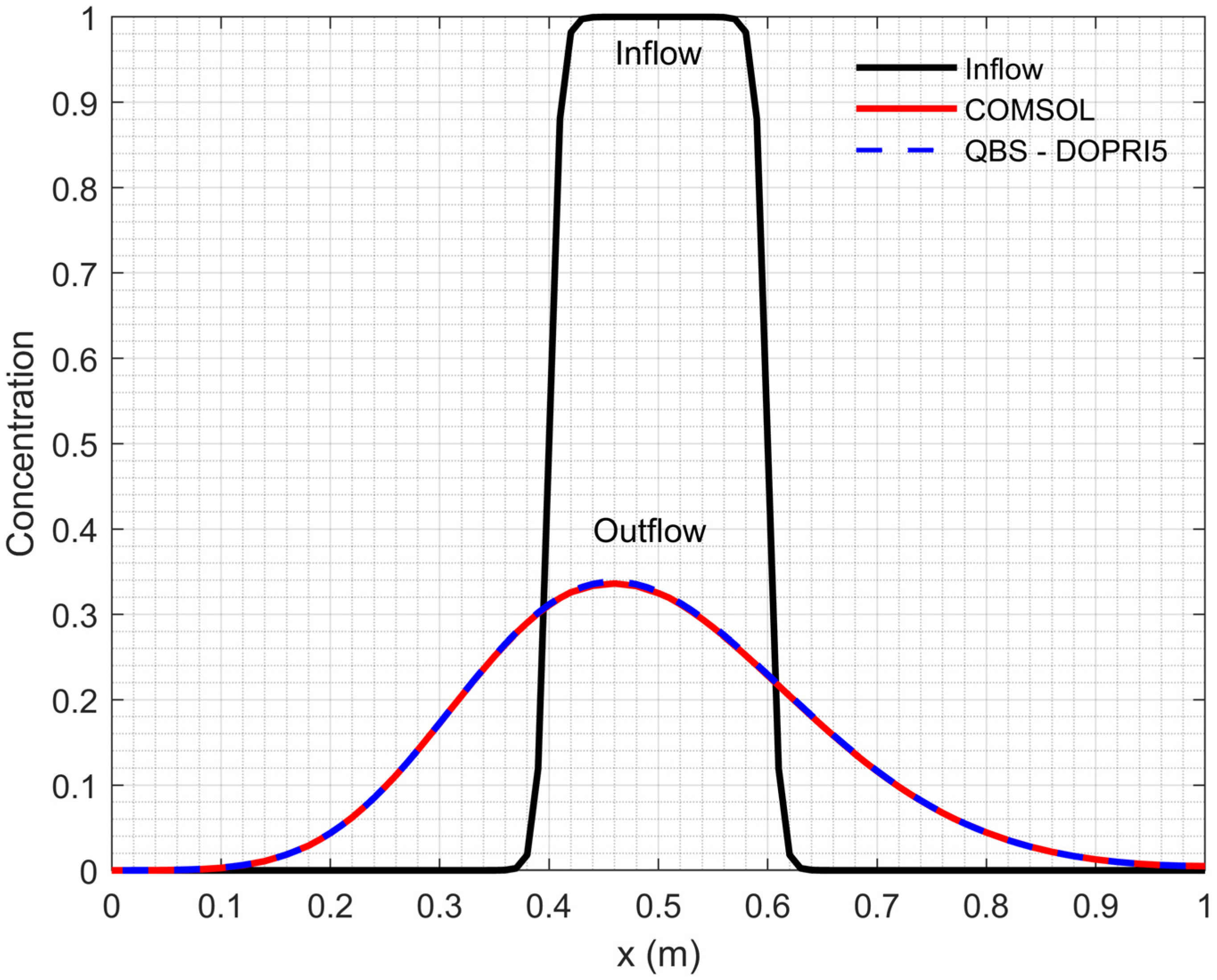
Moreover, the concentration profiles at the inlet and outlet boundaries, which are taken from the obtained solutions, are illustrated in Figure 10 and Figure 11, respectively. The effects of scenarios A and B conditions on contaminant transport are clearly seen in Figure 10 and Figure 11. It is clear that the QBS-DOPRI5 and COMSOL Multiphysics solutions are in good agreement for both scenarios. Also, COMSOL Multiphysics output results used to plot Figure 8 and Figure 9 are presented in Tables S2 and S3 file in Supplementary Materials, respectively. Moreover, the numerical values of the concentration profiles at the open boundary are presented separately in Table 9 for both scenarios.

5. Conclusions

In this paper, a new method of line approach based on B-spline functions is proposed for accurate simulation of two-dimensional contaminant transport problems. In the proposed method, quintic B-spline functions were used to approximate spatial derivatives. After the approximation of spatial derivatives, the partial differential equation representing the contaminant transport problem was converted to a time-dependent ordinary differential equation at each grid point. The system of ordinary differential equation system obtained for all grid points was solved with an adaptive time-integration scheme called DOPRI5. The biggest advantage of the proposed method is to convert the governing partial differential equation to the ordinary differential equation system and to obtain accurate solutions in an easier way and in a shorter time than conventional numerical methods such as finite difference, finite element, etc.
In this study, four numerical applications were carried out. The first two examples have analytical solutions, and the success of the proposed method on these examples is compared with the results of the studies available in the literature. As a result of this comparison, it was seen that the results obtained with QBS-DOPRI5 were compatible with analytical solutions and produced better results than other studies except for the compact finite difference method. In the third example, a hypothetical aquifer model with homogeneous and anisotropic dispersion coefficients without an analytical solution is solved. In order to question the quality of the results of the QBS-DOPRI5 model, the FDM-DOPRI5 model, which has an extremely high number of grids and can be considered almost an analytical solution, was used as a reference solution. In this example, the results of the proposed method are compared with the results obtained with the BEM and MLPG-MLS methods. As a result of this comparison, it has been determined that the proposed method produces the same results as the reference solution, whereas the solutions obtained by the BEM and MLPG-MLS methods are far from the reference solution. It is observed that the proposed method is approximately 1000 times faster than the FDM-DOPRI5 method, provided that the solution with the same accuracy is obtained. In addition, in order to test the reliability of the reference solution, this problem was solved with the COMSOL Multiphysics program. It should be noted that the adaptive mesh refinement property has been activated in the COMSOL Multiphysics program, and a large number of triangular elements have been used.
As is well known by groundwater hydrologists, aquifer parameters such as permeability and dispersivity can vary significantly in field conditions. Therefore, anisotropic dispersion with spatially varying velocity field was taken into account in the last example to question the usability of the proposed method in real applications. Since this example also does not have an analytical solution, a reference solution for determining the quality of QBS-DOPRI5 results was obtained with the help of the COMSOL Multiphysics program. For this example, two different scenarios have been created, and the results obtained with the proposed method under both scenarios are considered to be quite accurate and can be used safely in real applications. The proposed method of lines approach uses uniform mesh in space and adaptive mesh in time. Especially in the case of contaminant transport problems with sharp front, non-uniform mesh or adaptive mesh should be preferred in the space. By making a small modification in the code, these mesh structures can be easily created. The proposed method can also be used easily in the solution of three-dimensional contaminant transport problems and does not cause any changes in the solution algorithm. In addition, it can be safely preferred for the solution of engineering problems involving many partial differential equations due to the simplicity of the solution algorithm. The authors are planning to use the proposed method in several groundwater management problems.

Supplementary Materials

The following are available online at https://www.mdpi.com/2073-4441/12/6/1607/s1, Table S1: Figure 7 Comsol Multiphysics Output Result, Table S2: Figure 8 Comsol Multiphysics Output Result, Table S3: Figure 9 Comsol Multiphysics Output Result.

Author Contributions

Methodology, E.B. and G.G.; software, E.B. and G.G.; validation, E.B. and G.G.; writing—original draft preparation, E.B.; writing—review and editing, G.G.; supervision, G.G. All authors have read and agreed to the published version of the manuscript.

Funding

This research received no external funding.

Acknowledgments

In this study, a part of the first author’s PhD thesis study is presented.

Conflicts of Interest

The authors declare no conflict of interest.

Appendix A

Calculation of δ j , i ( t ) and γ j , i ( t ) values using known concentration values and Quintic B-spline functions are given below. Equations (A1–A3) and Equations (A4–A6) give approximations for x - and y -directions, respectively.
C ˜ ( x i , y j , t ) = δ j , i + 2 + 26 δ j , i + 1 + 66 δ j , i + 26 δ j , i 1 + δ j , i 2 j = 0 , 1 , , M
x C ˜ ( x i , y j , t ) = 5 ( δ j , i + 2 + 10 δ j , i + 1 10 δ j , i 1 δ j , i 2 ) j = 0 , 1 , , M
x 2 C ˜ ( x i , y j , t ) = 20 ( δ j , i + 2 + 2 δ j , i + 1 6 δ j , i + 2 δ j , i 1 + δ j , i 2 ) j = 0 , 1 , , M
C ˜ ( x i , y j , t ) = γ j + 2 , i + 26 γ j + 1 , i + 66 γ j , i + 26 γ j 1 , i + γ j 2 , i i = 0 , 1 , , N
y C ˜ ( x i , y j , t ) = 5 ( γ j + 2 , i + 10 γ j + 1 , i 10 γ j 1 , i γ j 2 , i ) i = 0 , 1 , , N
y 2 C ˜ ( x i , y j , t ) = 20 ( γ j + 2 , i + 2 γ j + 1 , i 6 γ j , i + 2 γ j 1 , i + γ j 2 , i ) i = 0 , 1 , , N
C ˜ ( x i , y j , t ) equals to initial concentration values at each time step. The δ j , i ( t ) and γ j , i ( t ) parameter matrix can be determined by using the relations given in Equations (A1) and (A4), which give N + 1 equations with N + 5 unknowns for each row and M + 1 equations with M + 5 unknowns for each column. The unknowns are δ j , 2 ,   δ j , 1 ,   δ j , N + 1 ,   δ j , N + 2 for each row vector and γ 2 , i ,   γ 1 , i ,   γ M + 1 , i ,   γ M + 2 , i for each column vector. To express them in terms of known parameters first and second derivatives are used at the boundary nodes. These derivatives are approximated by using finite difference (FD) schemes or known from boundary conditions depending on the problem domain.
C ( x 0 , y j , t ) = f j , 1 j = 0 , 1 , , M
C ( x 0 , y j , t ) = F j , 1 j = 0 , 1 , , M
C ( x N , y j , t ) = f j , 2   j = 0 , 1 , , M
C ( x N , y j , t ) = F j , 2 j = 0 , 1 , , M
C ( x i , y 0 , t ) = g 1 , i i = 0 , 1 , , N
C ( x i , y 0 , t ) = G 1 , i i = 0 , 1 , , N
C ( x i , y M , t ) = g 2 , i   i = 0 , 1 , , N
C ( x i , y M , t ) = G 2 , i i = 0 , 1 , , N
where f , F , g , G are boundary matrices consisting of first and second derivatives as scalar values, either calculated from FD schemes or known from boundary conditions. From Equations (A2–A3) and (A7–A10) following relations can be written.
f j , 1 = ( 5 / x ) ( δ j , 2 + 10 δ j , 1 10 δ j , 1 δ j , 2 )
f j , 2 = ( 5 / x ) ( δ j , N + 2 + 10 δ j , N + 1 10 δ j , N 1 δ j , N 2 )
F j , 1 = ( 20 / x 2 ) ( δ j , 2 + 2 δ j , 1 6 δ j , 0 + 2 δ j , 1 + δ j , 2 )
F j , 2 = ( 20 / x 2 ) ( δ j , N + 2 + 2 δ j , N + 1 6 δ j , N + 2 δ j , N 1 + δ j , N 2 )
From Equations (A15–A18) unknown parameters δ j , 2 ,   δ j , 1 ,   δ j , N + 1 ,   δ j , N + 2 can be obtained in terms of known parameters. The δ j , i ( t ) parameter matrix is then determined by solving the matrix system given below for j = 0 , 1 , , M .
[ 54 60 6 0 0 0 0 0 0 101 4 135 2 105 4 1 0 0 0 0 0 1 26 66 26 1 0 0 0 0 0 1 26 66 26 1 0 0 0 0 0 0 0 0 0 0 1 26 66 26 1 0 0 0 0 0 1 26 66 26 1 0 0 0 0 0 1 105 4 135 2 101 4 0 0 0 0 0 0 6 60 54 ] [ δ j , 0 ( t ) δ j , 1 ( t ) . . δ j , N 1 ( t ) δ j , N ( t ) ] = [ C ( x 0 , y j , t ) C ( x 1 , y j , t ) . . C ( x N 1 , y j , t ) C ( x N , y j , t ) ] + [ ( 3 / 5 ) f j , 1 Δ x + ( 1 / 10 ) F j , 1 Δ x 2 ( 1 / 40 ) f j , 1 Δ x + ( 1 / 160 ) F j , 1 Δ x 2 0 . 0 ( 1 / 40 ) f j , 2 Δ x + ( 1 / 160 ) F j , 2 Δ x 2 ( 3 / 5 ) f j , 2 Δ x + ( 1 / 10 ) F j , 2 Δ x 2 ]
From Equations (A5–A6) and (A11–A14) following relations can be written.
g 1 , i = ( 5 / y ) ( γ 2 , i + 10 γ 1 , i 10 γ 1 , i γ 2 , i )
g 2 , i = ( 5 / y ) ( γ M + 2 , i + 10 γ M + 1 , i 10 γ M 1 , i γ M 2 , i )
G 1 , i = ( 20 / y 2 ) ( γ 2 , i + 2 γ 1 , i 6 γ 0 , i + 2 γ 1 , i + γ 2 , i )
G 2 , i = ( 20 / y 2 ) ( γ M + 2 , i + 2 γ M + 1 , i 6 γ M , i + 2 γ M 1 , i + γ M 2 , i )
From the formulations in Equations (A20–A23) the unknown parameters γ 2 , i ,   γ 1 , i ,   γ M + 1 , i ,   γ M + 2 , i can be determined in terms of known parameters. By using these relations, the γ j , i matrix can be calculated by solving the matrix system given below for i = 0 , 1 , , N .
[ 54 60 6 0 0 0 0 0 0 101 4 135 2 105 4 1 0 0 0 0 0 1 26 66 26 1 0 0 0 0 0 1 26 66 26 1 0 0 0 0 0 0 0 0 0 0 1 26 66 26 1 0 0 0 0 0 1 26 66 26 1 0 0 0 0 0 1 105 4 135 2 101 4 0 0 0 0 0 0 6 60 54 ] [ γ 0 , i ( t ) γ 1 , i ( t ) . . γ M 1 , i ( t ) γ M , i ( t ) ] = [ C ( x i , y 0 , t ) C ( x i , y 1 , t ) . . C ( x i , y M 1 , t ) C ( x i , y M , t ) ] + [ ( 3 / 5 ) g 1 , i Δ y + ( 1 / 10 ) G 1 , i Δ y 2 ( 1 / 40 ) g 1 , i Δ y + ( 1 / 160 ) G 1 , i Δ y 2 0 . 0 ( 1 / 40 ) g 2 , i Δ y + ( 1 / 160 ) G 2 , i Δ y 2 ( 3 / 5 ) g 2 , i Δ y + ( 1 / 10 ) G 2 , i Δ y 2 ]
Consequently, the first and second derivatives in x - and y -directions at each nodal point can be calculated by using Equations (A2–A3) and (A5–A6), respectively since the parameter matrices are known.

References

  1. Sun, N.Z. Mathematical Modeling of Groundwater Pollution; Springer: New York, NY, USA, 1996. [Google Scholar] [CrossRef]
  2. Wang, H.F.; Anderson, M.P. Introduction to Groundwater Modeling: Finite Difference and Finite Element Methods; Academic Press: San Diego, CA, USA, 1982. [Google Scholar] [CrossRef]
  3. Tatalovich, M.E.; Lee, K.Y.; Chrysikopoulos, C.V. Modeling the transport of contaminants originating from the dissolution of DNAPL pools in aquifers in the presence of dissolved humic substances. Transp. Porous Media 2000, 38, 93–115. [Google Scholar] [CrossRef]
  4. Noye, B.; Tan, H. Finite difference methods for solving the two-dimensional advection–diffusion equation. Int. J. Numer. Methods Fluids 1989, 9, 75–98. [Google Scholar] [CrossRef]
  5. Ataie-Ashtiani, B.; Lockington, D.A.; Volker, R.E. Numerical correction for finite-difference solution of the advection—Dispersion equation with reaction. J. Contam. Hydrol. 1996, 23, 149–156. [Google Scholar] [CrossRef]
  6. Dehghan, M. Weighted finite difference techniques for the one-dimensional advection-diffusion equation. Appl. Math. Comput. 2004, 147, 307–319. [Google Scholar] [CrossRef]
  7. Sheu, T.W.H.; Chen, Y.H. Finite element analysis of contaminant transport in groundwater. Appl. Math. Comput. 2002, 127, 23–43. [Google Scholar] [CrossRef]
  8. Badrot-Nico, F.; Brissaud, F.; Guinot, V. A finite volume upwind scheme for the solution of the linear advection-diffusion equation with sharp gradients in multiple dimensions. Adv. Water Resour. 2007, 30, 2002–2025. [Google Scholar] [CrossRef]
  9. Eldho, T.I.; Vasudeva Rao, B. Simulation of two-dimensional contaminant transport with dual reciprocity boundary elements. Eng. Anal. Bound. Elem. 1997, 20, 213–228. [Google Scholar] [CrossRef]
  10. Mittal, R.C.; Jain, R.K. Numerical solution of convection-diffusion equation using cubic B-splines collocation methods with Neumann’ s boundary conditions. Int. J. Appl. Math. Comput. 2012, 4, 115–127. [Google Scholar]
  11. Boddula, S.; Eldho, T.I. A moving least squares based meshless local petrov-galerkin method for the simulation of contaminant transport in porous media. Eng. Anal. Bound. Elem. 2017, 78, 8–19. [Google Scholar] [CrossRef]
  12. Meenal, M.; Eldho, T.I. Two-dimensional contaminant transport modeling using meshfree point collocation method (PCM). Eng. Anal. Bound. Elem. 2012, 36, 551–561. [Google Scholar] [CrossRef]
  13. Bahar, E.; Gürarslan, G. Numerical solution of advection-diffusion equation using operator splitting method. Int. J. Eng. Appl. Sci. 2017, 9, 76–88. [Google Scholar] [CrossRef] [Green Version]
  14. Gurarslan, G.; Karahan, H.; Alkaya, D.; Sari, M.; Yasar, M. Numerical solution of advection-diffusion equation using a sixth-order compact finite difference method. Math. Probl. Eng. 2013, 2013, 672936. [Google Scholar] [CrossRef] [Green Version]
  15. Gurarslan, G. Accurate simulation of contaminant transport using high-order compact finite difference schemes. J. Appl. Math. 2014, 2014, 396738. [Google Scholar] [CrossRef]
  16. Zhou, J.G. A lattice boltzmann method for solute transport. Int. J. Numer. Methods Fluids 2009, 61, 848–863. [Google Scholar] [CrossRef]
  17. Perko, J. A single-relaxation-time lattice Boltzmann model for anisotropic advection-diffusion equation based on the diffusion velocity flux formulation. Comput. Geosci. 2018, 22, 1423–1432. [Google Scholar] [CrossRef]
  18. Korkmaz, A.; Dağ, İ. Cubic B-spline differential quadrature methods for the advection-diffusion equation. Int. J. Numer. Methods Heat Fluid Flow 2012, 22, 1021–1036. [Google Scholar] [CrossRef]
  19. Irk, D.; Dağ, İ.; Tombul, M. Extended cubic B-spline solution of the advection-diffusion equation. KSCE J. Civ. Eng. 2015, 19, 929–934. [Google Scholar] [CrossRef]
  20. Dhawan, S.; Kapoor, S.; Kumar, S. Numerical method for advection diffusion equation using FEM and B-splines. J. Comput. Sci. 2012, 3, 429–437. [Google Scholar] [CrossRef]
  21. Korkmaz, A.; Dağ, I. Quartic and quintic B-spline methods for advection–diffusion equation. Appl. Math. Comput. 2016, 274, 208–219. [Google Scholar] [CrossRef]
  22. Nazir, T.; Abbas, M.; Izani, A.; Abd, A. The numerical solution of advection—Diffusion problems using new cubic trigonometric B-splines approach. Appl. Math. Model. 2016, 40, 4586–4611. [Google Scholar] [CrossRef]
  23. Mohammadi, R. Exponential B-Spline solution of convection-diffusion equations. Appl. Math. 2013, 4, 33152. [Google Scholar] [CrossRef] [Green Version]
  24. Mittal, R.C.; Tripathi, A. Numerical solutions of two-dimensional unsteady convection–diffusion problems using modified bi-cubic B-spline finite elements. Int. J. Comput. Math. 2017, 94, 1–21. [Google Scholar] [CrossRef]
  25. Rohila, R.; Mittal, R.C. An efficient Bi-cubic B-spline ADI method for numerical solutions of two-dimensional unsteady advection diffusion equations. Int. J. Numer. Methods Heat Fluid Flow 2018, 28, 2620–2649. [Google Scholar] [CrossRef]
  26. Shukla, H.S.; Tamsir, M. An exponential cubic B-spline algorithm for multi-dimensional convection-diffusion equations. Alexandria Eng. J. 2018, 57, 1999–2006. [Google Scholar] [CrossRef]
  27. Dormand, J.R.; Prince, P.J. A family of embedded Runge-Kutta formulae. J. Comput. Appl. Math. 1980, 6, 19–26. [Google Scholar] [CrossRef] [Green Version]
  28. Bear, J.; Cheng, A.H.-D. Modeling Groundwater Flow and Contaminant Transport; Springer: Berlin, Germany, 2010. [Google Scholar] [CrossRef]
  29. Mittal, R.C.; Arora, G. Quintic B-spline collocation method for numerical solution of the Kuramoto-Sivashinsky equation. Commun. Nonlinear Sci. Numer. Simul. 2010, 15, 2798–2808. [Google Scholar] [CrossRef]
  30. Hamdi, S.; Schiesser, W.; Griffiths, G. Method of lines. Scholarpedia 2007, 2, 2859. [Google Scholar] [CrossRef]
  31. Fehlberg, E. Low Order Classical Runge Kutta Formulas with Stepwise Control and Their Application to Some Heat Transfer Problems. 1969. Available online: https://ntrs.nasa.gov/search.jsp?R=19690021375 (accessed on 1 June 2020).
  32. Shampine, L.F. Some practical Runge-Kutta formulas. Math. Comput. 1986, 46, 135–150. [Google Scholar] [CrossRef]
  33. Butcher, J.C. Implicit runge-kutta processes. Math. Comput. 1964, 18, 50–64. [Google Scholar] [CrossRef]
  34. Kalita, J.C.; Dalal, D.C.; Dass, A.K. A class of higher order compact schemes for the unsteady two-dimensional convection-diffusion equation with variable convection coefficients. Int. J. Numer. Methods Fluids 2002, 38, 1111–1131. [Google Scholar] [CrossRef]
  35. Dehghan, M.; Mohebbi, A. High-order compact boundary value method for the solution of unsteady convection-diffusion problems. Math. Comput. Simul. 2008, 79, 683–699. [Google Scholar] [CrossRef]
  36. Karaa, S.; Zhang, J. High order ADI method for solving unsteady convection-diffusion problems. J. Comput. Phys. 2004, 198, 1–9. [Google Scholar] [CrossRef]
  37. Tian, Z.F.; Ge, Y.B. A fourth-order compact ADI method for solving two-dimensional unsteady convection-diffusion problems. J. Comput. Appl. Math. 2007, 198, 268–286. [Google Scholar] [CrossRef] [Green Version]
  38. Wexler, E.J. Analytical Solutions for One-, Two-, and Three-Dimensional Solute Transport in Ground-Water Systems with Uniform Flow; United State Goverment Printing Office: Washington, DC, USA, 1992.
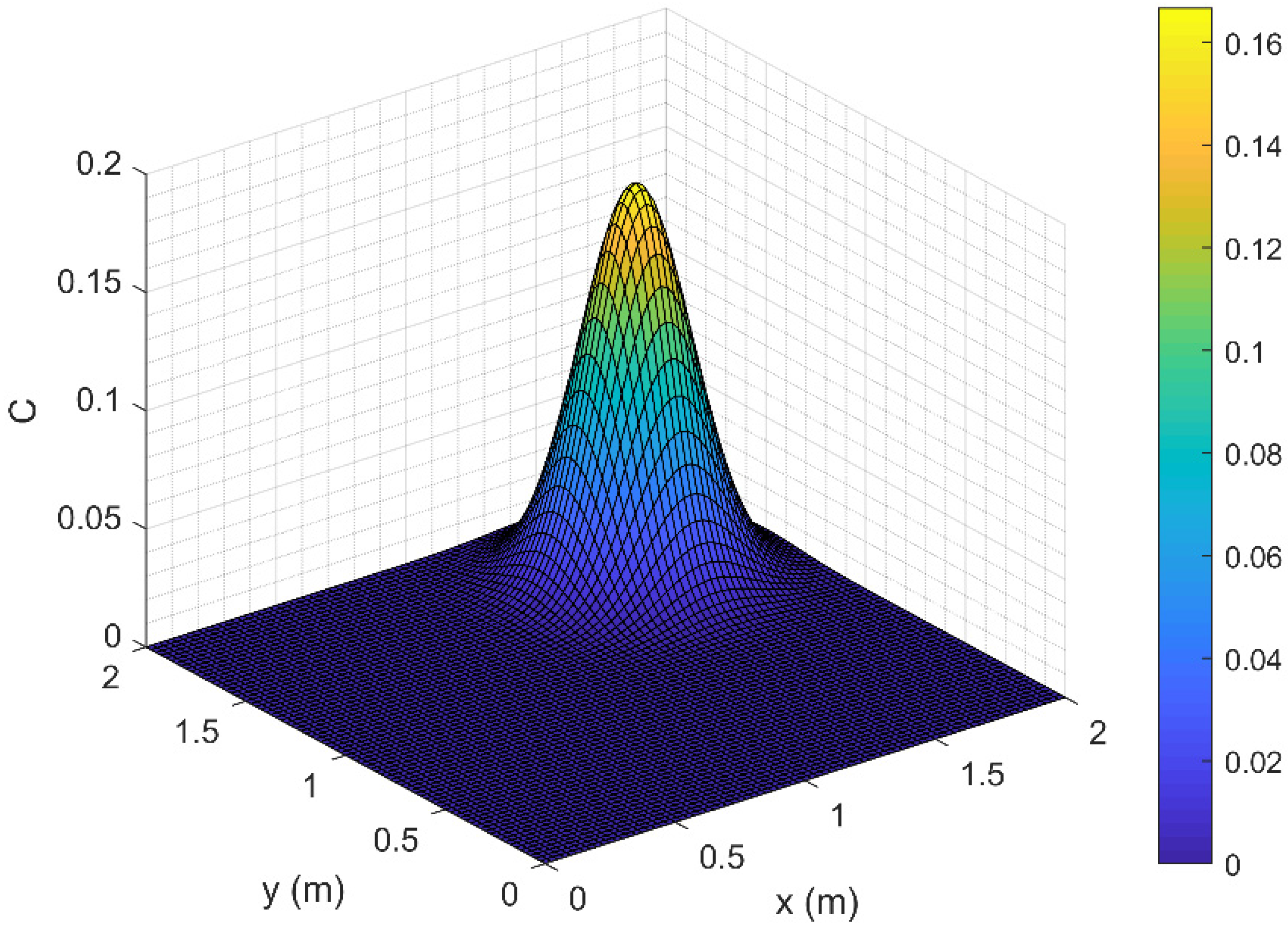
Figure 1. Approximate solution obtained with QBS-DOPRI5 at time t = 1.25   s with x = y = 0.025   m , V x = V y = 0.8   m / s , D x x = D y y = 0.01   m 2 / s .
Water 12 01607 g001
Figure 2. Contour plot of the analytical solution and numerical solution.
Water 12 01607 g002
Figure 3. Comparison of approximate solution obtained with QBS-DOPRI5 and analytical solution at time = 1500   days ( x = 20   m ,   y = 16   m ) .
Water 12 01607 g003
Figure 4. Comparison of approximate solution obtained with QBS-DOPRI5 and analytical solution at time = 3000   days ( x = 20   m ,   y = 16   m ) .
Water 12 01607 g004
Figure 5. Comparison of approximate solutions with analytical solutions for different simulation times at centerline.
Water 12 01607 g005
Figure 6. Comparison of approximate solutions obtained by QBS-DOPRI5 ( x = y = 5   m ) and Reference Solution ( x = y = 0.5   m ) .
Water 12 01607 g006
Figure 7. Comparison of approximate solutions obtained by QBS-DOPRI5 ( x = y = 5   m ) and COMSOL Multiphysics.
Water 12 01607 g007
Figure 8. Concentration field obtained by QBS-DOPRI5 ( x = y = 0.01   m ) and COMSOL Multiphysics at time 1.7 days for Scenario A.
Water 12 01607 g008
Figure 9. Concentration field obtained by QBS-DOPRI5 ( x = y = 0.01   m ) and COMSOL Multiphysics at time 1.7 days for Scenario B.
Water 12 01607 g009
Figure 10. Concentration profiles at the inlet and outlet boundary at time 1.7 days for Scenario A.
Water 12 01607 g010
Figure 11. Concentration profiles at the inlet and outlet boundary at time 1.7 days for Scenario B.
Water 12 01607 g011
Table 1. The values of B i ( x ) and its derivatives at nodal points.
x x i 3 x i 2 x i 1 x i x i + 1 x i + 2 x i + 3
B i ( x ) 0 1 26 66 26 1 0
B i ( x ) 0 5 / x 50 / x 0 50 / x 5 / x 0
B i ( x ) 0 20 / x 2 40 / x 2 120 / x 2 40 / x 2 20 / x 2 0
Table 2. The values of Q j ( y ) and its derivatives at nodal points.
y y j 3 y j 2 y j 1 y j y j + 1 y j + 2 y j + 3
Q j ( y ) 0 1 26 66 26 1 0
Q j ( y ) 0 5 / y 50 / y 0 50 / y 5 / y 0
Q j ( y ) 0 20 / y 2 40 / y 2 120 / y 2 40 / y 2 20 / y 2 0
Table 3. Butcher array for DOPRI5.
ω ϕ
0 0
1 5 1 5 0
3 10 3 40 9 40 0
4 5 44 45 56 15 32 9 0
8 9 19372 6561 25360 2187 64448 6561 212 729 0
1 9017 3168 355 33 46732 5247 49 176 5103 18656 0
1 35 384 0 500 1113 125 192 2187 6784 11 84
ψ T 35 384 0 500 1113 125 192 2187 6784 11 84 0
ψ ^ T 5179 57600 0 7571 16695 393 640 92097 339200 187 2100 1 40
Table 4. Average absolute error values obtained in Example 1 at the time t = 1 s over the domain [1,2] × [1,2] with Vx = Vy = 0.8 m/s and Dxx = Dyy = 0.005 m2/s.
x = y Dehghan and Mohebbi [35]Mittal and Tripathi [24]QBS-DOPRI5
0.04 2.7414 × 10 4 1.0378 × 10 6 1.0218 × 10 6
0.02 2.0043 × 10 5 6.5768 × 10 8 5.0215 × 10 8
0.01 1.3043 × 10 6 3.8352 × 10 9 2.9706 × 10 9
Table 5. Comparison of average absolute error and maximum absolute error values obtained at the time t = 1.25 s over the domain [0,2] × [0,2] with Vx = Vy = 0.8 m/s.
References D x x = D y y = 0.01   m 2 / s D x x = D y y = 0.001   m 2 / s
Average ErrorMaximum ErrorAverage ErrorMaximum Error
Noye and Tan [4] 1.430 × 10 5 4.840 × 10 4 --
Kalita et al. [34] 1.590 × 10 5 4.447 × 10 4 --
Karaa and Zhang [36] 9.218 × 10 6 2.500 × 10 4 --
Tian and Ge [37] 9.663 × 10 6 2.664 × 10 4 --
Dehghan and Mohebbi [35] 9.483 × 10 6 2.469 × 10 4 --
Shukla and Tamsir [26] 6.482 × 10 7 1.609 × 10 6 --
Gurarslan MC-CD6 [15] 2.600 × 10 5 7.920 × 10 3 --
Gurarslan RK4-CD6 [15] 2.240 × 10 8 1.650 × 10 5 --
Mittal and Tripathi [24] 1.021 × 10 7 9.110 × 10 4 2.120 × 10 8 1.417 × 10 4
QBS-DOPRI5 1.224 × 10 7 1.301 × 10 5 2.842 × 10 6 5.141 × 10 4
Table 6. Comparison of concentration values obtained by QBS-DOPRI5 with other numerical methods at time t = 200   days (Scenario A).
Location
( x , y )
BEM
[9]
MLPG-MLS [11]
h = 25   m
MLPG-MLS [11]
h = 5   m
QBS-DOPRI5
h = 25   m
QBS-DOPRI5
h = 5   m
Reference Solution
h = 0.5   m
( 100 , 125 ) 0.7740.7710.7710.7670.7680.768
( 150 , 150 ) 0.7970.7940.7950.8240.8330.833
( 200 , 125 ) 0.3620.3610.3610.3910.3890.389
( 300 , 125 ) 0.0570.0560.0560.0580.0520.052
Table 7. Comparison of CPU times of QBS-DOPRI5 and FDM-DOPRI5 for different grid size and t = 200 days (Scenario A).
Method h   ( m ) Location   ( x , y ) CPU ( s )
( 100 , 125 ) ( 150 , 150 ) ( 200 , 125 ) ( 300 , 125 )
QBS-DOPRI5 25 0.7670.8240.3910.0580.57
25 / 2 0.7680.8310.3890.0531.40
25 / 4 0.7680.8330.3890.05219.57
25 / 8 0.7680.8330.3890.052278.17
25 / 16 0.7680.8330.3890.0529041.92
FDM-DOPRI5 25 0.8150.8670.4210.0740.31
25 / 2 0.7790.8450.3970.0570.38
25 / 4 0.7710.8360.3910.0531.05
25 / 8 0.7690.8340.3900.0528.38
25 / 16 0.7690.8330.3890.05284.04
25 / 32 0.7680.8330.3890.0521302.46
Reference Solution 0.50 0.7680.8330.3890.0528399.55
Table 8. Comparison of CPU times of QBS-DOPRI5 and FDM-DOPRI5 for different grid size and t = 200 days (Scenario B).
Method h   ( m ) Location   ( x , y ) CPU ( s )
( 100 , 125 ) ( 150 , 150 ) ( 200 , 125 ) ( 300 , 125 )
QBS-DOPRI5 25 0.7790.8520.3360.0260.76
25 / 2 0.7810.8610.3310.0231.97
25 / 4 0.7820.8640.3300.02226.08
25 / 8 0.7820.8640.3300.022479.95
FDM-DOPRI5 25 0.8440.8950.3780.0450.37
25 / 2 0.8040.8800.3450.0270.47
25 / 4 0.7910.8710.3370.0231.25
25 / 8 0.7860.8670.3340.02210.08
25 / 16 0.7840.8660.3320.02297.03
25 / 32 0.7830.8650.3310.0221532.50
25 / 64 0.7820.8640.3300.02227691.71
Reference Solution 0.25 0.7820.8640.3300.022174576.14
Table 9. QBS-DOPRI5 and COMSOL Multiphysics outflow results at different x coordinates.
x ( m ) Scenario A Scenario B
QBS-DOPRI5COMSOLQBS-DOPRI5COMSOL
0.10 0.0030.0030.0000.000
0.20 0.0440.0430.0000.000
0.30 0.1730.1720.0020.000
0.35 0.2510.2510.0480.055
0.40 0.3120.3110.4850.486
0.45 0.3380.3350.8750.864
0.50 0.3270.3250.8980.898
0.55 0.2860.2850.8060.799
0.60 0.2290.2280.4260.426
0.65 0.1700.1690.0800.088
0.70 0.1170.1160.0080.008
0.80 0.0440.0440.000-0.001
0.90 0.0130.0130.0000.000