A Fully Implicit Finite Volume Scheme for a Seawater Intrusion Problem in Coastal Aquifers


Abstract
1. Introduction
2. Mathematical Model
3. Numerical Scheme
4. Numerical Simulations
4.1. DuMu: Numerical Simulator
4.2. Numerical Tests
4.3. Test 1: A Field-Scale Free Aquifer
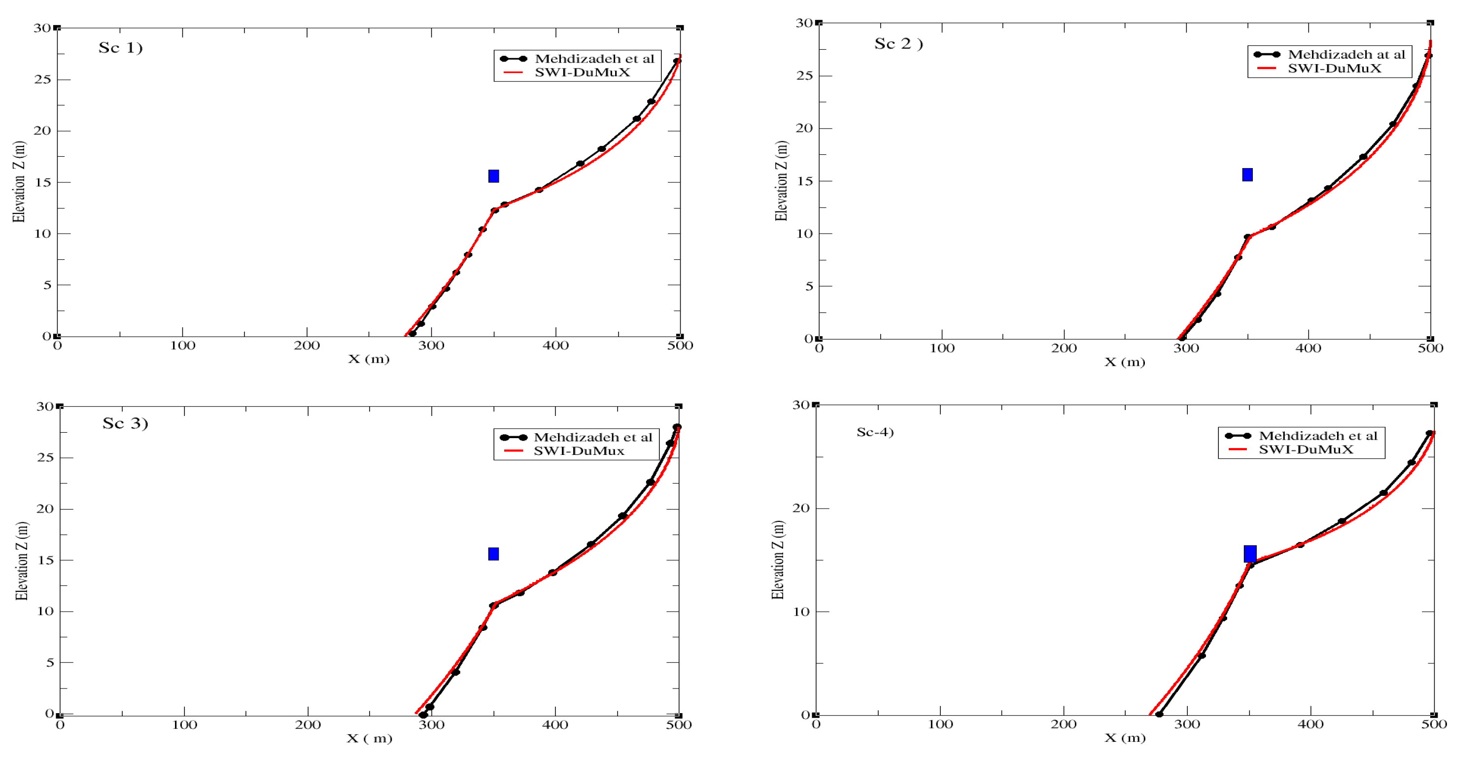
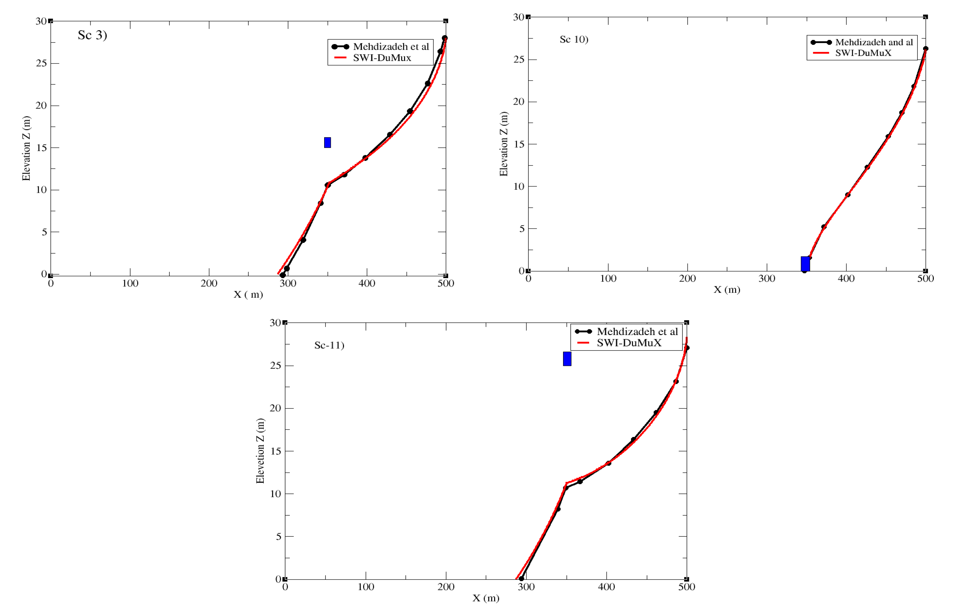
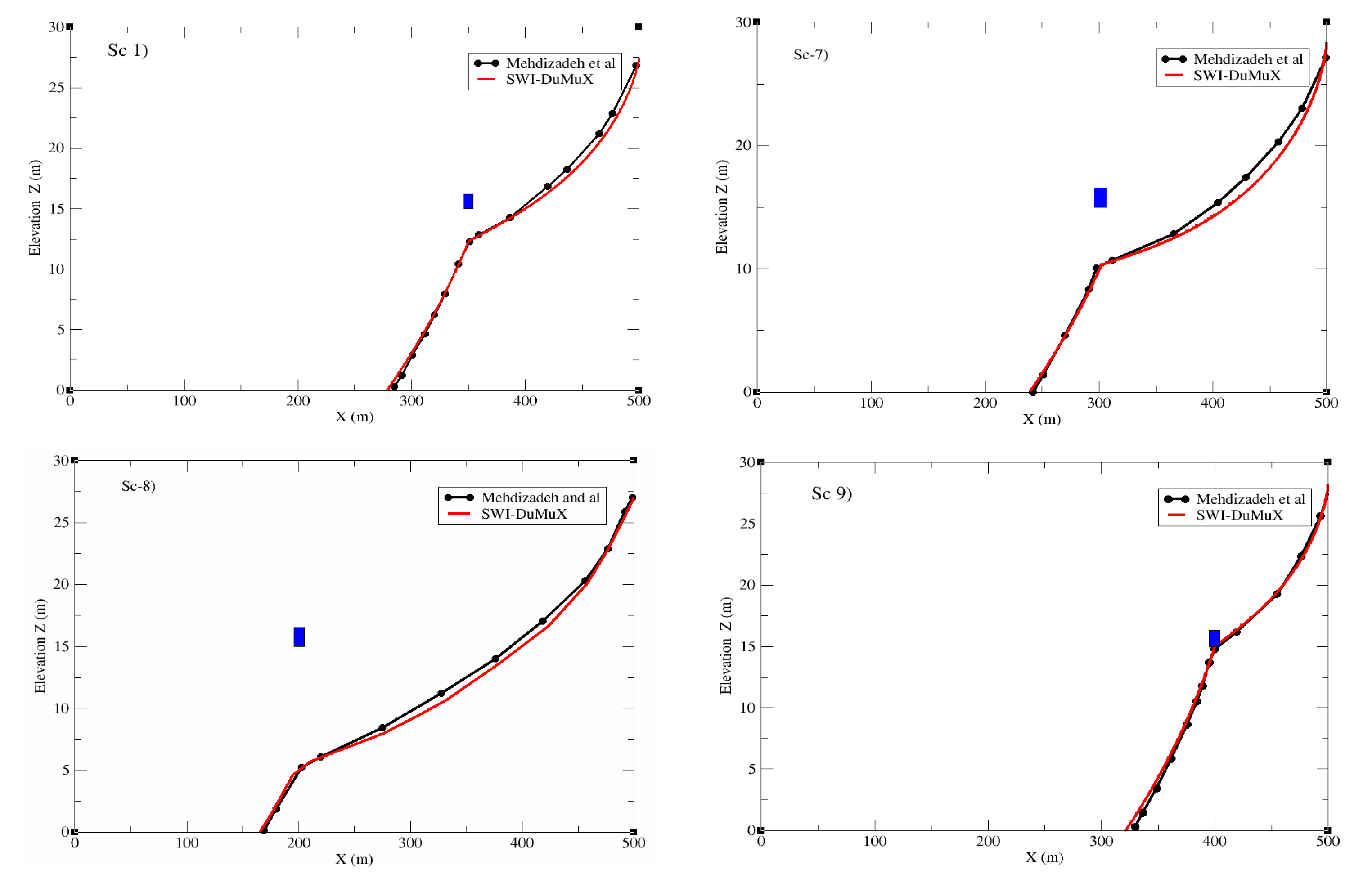
4.3.1. Numerical Results by Varying the Pumping Rate
4.3.2. Numerical Results by Varying the Depth of the Well
4.3.3. Numerical Results by Varying the Longitudinal Position of the Well
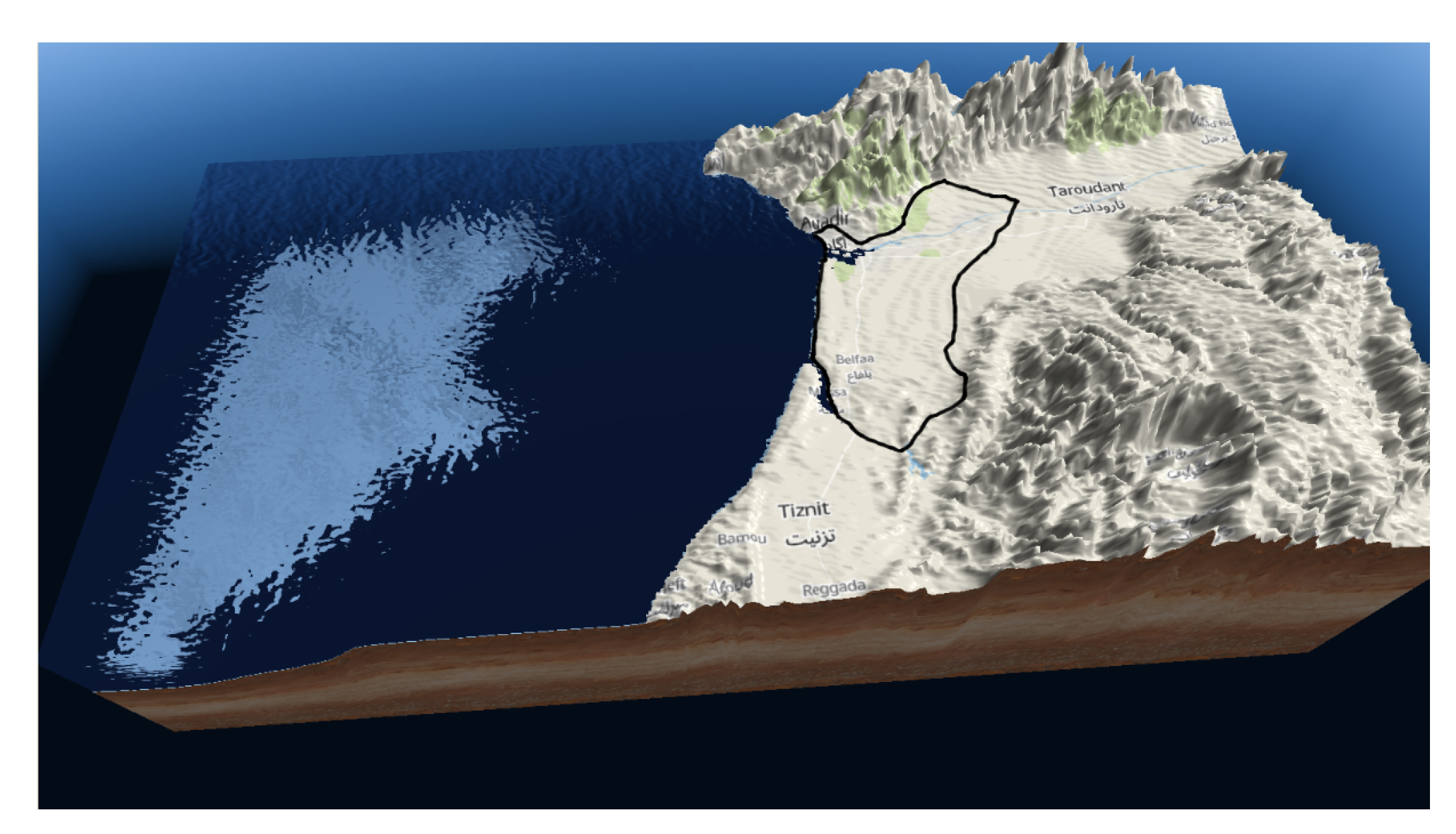
4.4. Test 2: Souss–Chtouka Aquifer Field Case
4.4.1. Geographic Location and Geologic Settings
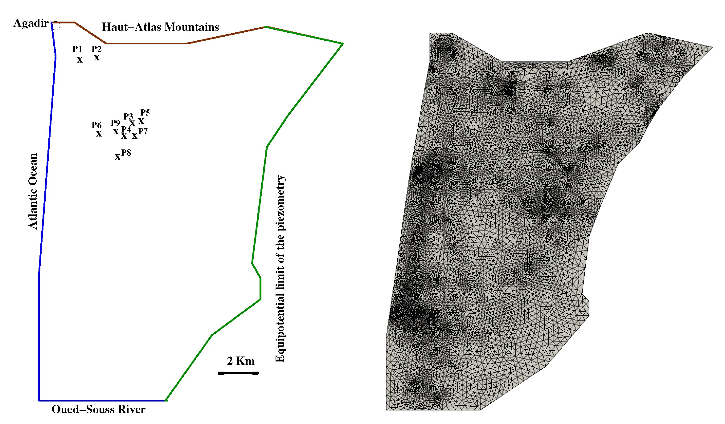
4.4.2. Studied Domain and Discretization
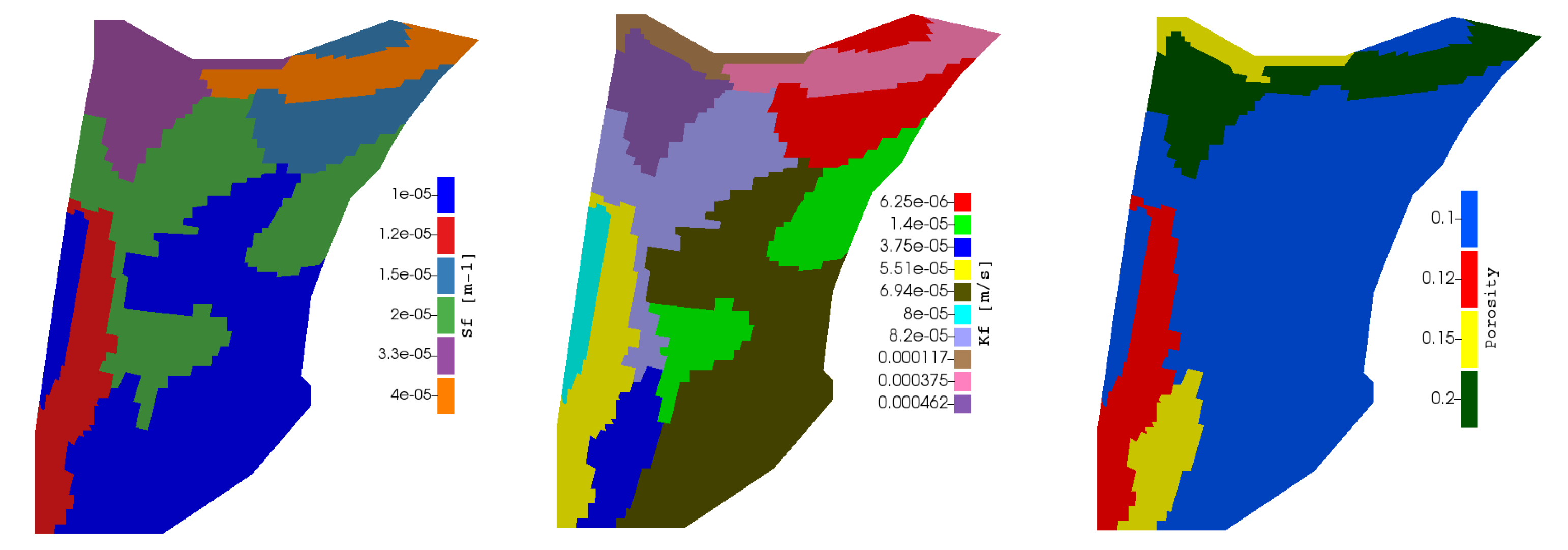
4.4.3. Parameters and Boundary Conditions
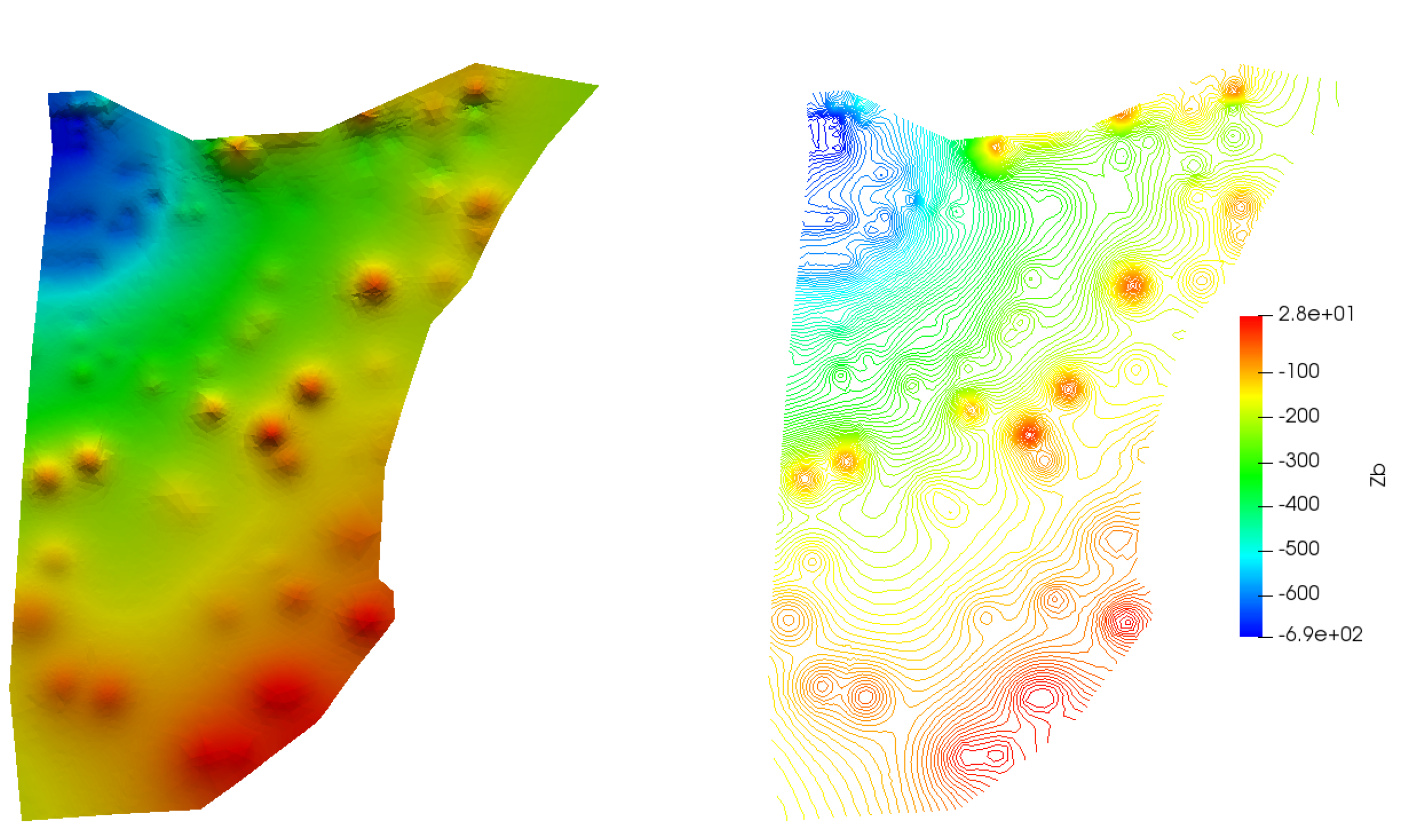
4.4.4. Numerical Results
5. Conclusions
Author Contributions
Funding
Acknowledgments
Conflicts of Interest
References
- Bear, J.; Cheng, A.H.D. Modeling Groundwater Flow and Contaminant Transport; Springer: Dordrecht, The Netherlands, 2000. [Google Scholar]
- Bear, J.; Cheng, A.H.D.; Sorek, S.; Ouazar, D.; Herrera, I. Seawater Intrusion in Coastal Aquifers, Concepts, Methods and Practices; Kluwer Academic Publishers: Dordrecht, The Netherlands, 1999. [Google Scholar]
- Bear, J.; Verruijt, A. Modelling Groundwater Flow and Pollution; D. Reidel Publishing Company: Dordrecht, The Netherlands, 1987. [Google Scholar]
- Cheng, A.H.D. Multilayered Aquifier Systems. In Fundamentals and Applications; CRC Press Published: New York, NY, USA, 2000. [Google Scholar]
- Cheng, A.H.D.; Ouazar, D. Coastal Aquifer Management-Monitoring, Modeling, and Case Studies; CRC Press: New York, NY, USA; Washington, DC, USA, 2003. [Google Scholar]
- Diersch, H.-J.G.G. FEFLOW: Finite Element Modeling of Flow, Mass and Heat Transport in Porous and Fractured Media; Springer: Berlin/Heidelberg, Germany, 2014. [Google Scholar]
- Bobba, G.H. Mathematical models for saltwater intrusion in coastal aquifers. Water Resour. Manag. 1993, 7, 3–37. [Google Scholar] [CrossRef]
- Werner, A.D.; Bakke, M.; Post, V.E.A.; Vandenbohede, A.; Barry, D.A. Seawater intrusion processes, investigation and management: Recent advances and future challenges. Adv. Water Resour. 2013, 51, 3–26. [Google Scholar] [CrossRef]
- Cobaner, M.; Yurtal, R.; Dogan, A.; Motz, L.H. Three dimensional simulation of seawater intrusion in coastal aquifers: A case study in the Goksu Deltaic Plain. J. Hydrol. 2012, 464–465, 262–280. [Google Scholar] [CrossRef]
- Essaid, H.L. A multilayered sharp interface model of coupled freshwater and saltwater flow in coastal systems: Model developpement and application. Water Resour. Res. 1990, 26, 1431–1454. [Google Scholar] [CrossRef]
- Fahs, M.; Koohbor, B.; Belfort, B.; Ataie-Ashtiani, B.; Simmons, C.T.; Younes, A.; Ackerer, P. A generalized semi-analytical solution for the dispersive Henry problem: Effect of stratification and anisotropy on seawater intrusion. Water 2018, 10, 230. [Google Scholar] [CrossRef]
- Houben, G.H.; Stoeckl, L.; Mariner, K.E.; Choudhury, A.S. The influence of heterogeneity on coastal groundwater flow-physical and numerical modeling of fringing reefs, dykes and structured conductivity fields. Adv. Water Resour. 2017, 113, 155–166. [Google Scholar] [CrossRef]
- Huyakorn, P.S.; Wu, Y.S.; Park, N.S. Multiphase approach to the numerical solution of a sharp-interface saltwater intrusion problem. Water Resour. Res. 1996, 32, 93–102. [Google Scholar] [CrossRef]
- Povich, T.J.; Dawson, C.N.; Farthing, M.W.; Kees, C.E. Finite element methods for variable density flow and solute transport. Comput. Geosci. 2013, 17, 529–549. [Google Scholar] [CrossRef]
- Bouzouf, B.; Chen, Z. A comparison of finite volume method and sharp model for two dimensional saltwater intrusion modeling. Can. J. Civ. Eng. 2014, 41, 191–196. [Google Scholar] [CrossRef]
- Mehdizadeh, S.; Vafaie, F.; Abolghasemi, H. Assessment of sharp-interface approach for saltwater intrusion prediction in an unconfined coastal aquifer exposed to pumping. Environ. Earth Sci. 2015, 73, 8345–8355. [Google Scholar] [CrossRef]
- Vafaie, F.; Mehdizadeh, S. Investigation of sea level rise effect on saltwater intrusion in an unconfined coastal aquifer using sharp-interface approach. Int. J. Glob. Warm. 2015, 8, 501–515. [Google Scholar] [CrossRef]
- Eymard, R.; Gallouët, T.; Herbin, R. Finite volume methods. In Handbook of Numerical Analysis; Ciarlet, P.G., Lions, J.L., Eds.; North-Holland: Amsterdam, The Netherlands, 2000; pp. 713–1022. [Google Scholar]
- DuMuX DUNE for Multi-{Phase, Component, Scale, Physics, ...} Flow and Transport in Porous Media. Available online: http://www.dumux.org (accessed on 1 June 2020).
- Flemisch, B.; Darcis, M.; Erbertseder, K.; Faigle, B.; Lauser, A.; Mosthaf, V.K.; Muthing, S.; Nuske, P.; Tatomir, A.; Wolf, M.; et al. DuMuX: Dune for multi-{Phase, Component, Scale, Physics, …} flow and transport in porous media. Adv. Water Resour. 2011, 34, 1102–1112. [Google Scholar] [CrossRef]
- DUNE, the Distributed and Unified Numerics Environment. Available online: https://www.dune-project.org (accessed on 1 June 2020).
- Abouelmahassine, N. Modélisation Préliminaire du Biseau salé par Éléments Finis dans la Zone Côtière de Souss–Chtouka. Master’s Thesis, Ecole Mohammadia d’Ingénieurs, Rabat, Morocco, 2002. [Google Scholar]
- Eymard, R.; Gallouët, T.; Guichard, C.; Herbin, R.; Masson, R. TP or not TP, that is the question. Comput. Geosci. 2014, 18, 285–296. [Google Scholar] [CrossRef]
- Linga, G.; Møyner, O.; Nilsen, H.M.; Moncorgé, A.; Lie, K.A. An implicit local time-stepping method based on cell reordering for multiphase flow in porous media. J. Comput. Phys. 2020, 100051. [Google Scholar] [CrossRef]
- Vohralik, M.; Wheeler, M.F. A posteriori error estimates, stopping criteria, and adaptivity for two-phase flows. Comput. Geosci. 2013, 17, 789–812. [Google Scholar] [CrossRef][Green Version]
- Younes, A.; Ackerer, P. Empirical versus time stepping with embedded error control for density-driven flow in porous media. Water Resour. Res. 2010, 46. [Google Scholar] [CrossRef]
- Ait Hammou Oulhaj, A. Numerical analysis of a finite volume scheme for a seawater intrusion model with cross-diffusion in an unconfined aquifer. Numer. Methods Partial Differ. Equ. 2018, 34, 857–880. [Google Scholar] [CrossRef]
- Keulegan, H.G. An Example Report on Model Laws for Density Current; U.S. National Bureau of Standards: Gaithersburg, MD, USA, 1954.
- Abudawia, A.; Rosier, C. Numerical analysis for a seawater intrusion problem in a confined aquifer. Math. Comput. Simul. 2015, 118, 2–16. [Google Scholar] [CrossRef]
- Marion, P.; Najib, K.; Rosier, C. Numerical simulations for a seawater intrusion problem in a free aquifer. Appl. Numer. Math. 2014, 75, 48–60. [Google Scholar] [CrossRef]
- Shi, L.; Cui, L.; Park, N.; Huyakorn, P.S. Applicability of a sharp-interface model for estimating steady-state salinity at pumping wells-validation against sand-tank experiments. Contam. Hydrol. 2011, 124, 35–42. [Google Scholar] [CrossRef]
- Choquet, C.; Diédhiou, M.; Rosier, C. Derivation of a sharp-diffuse interfaces model for seawater intrusion in a free aquifer, Numerical simulations. SIAM J. Appl. Math. 2016, 76, 138–158. [Google Scholar] [CrossRef]
- Cherfils, L.; Choquet, C.; Diédhiou, M. Numerical validation of an upscaled sharp-diffuse interface model for stratified miscible flows. Math. Comput. Simul. 2017, 137, 246–265. [Google Scholar] [CrossRef]
- Abudawia, A.; Mourad, A.; Rodrigues, J.H.; Rosier, C. A finite element method for a seawater intrusion problem in unconfined aquifers. Appl. Numer. Math. 2018, 127, 349–369. [Google Scholar] [CrossRef]


| Parameters | |
|---|---|
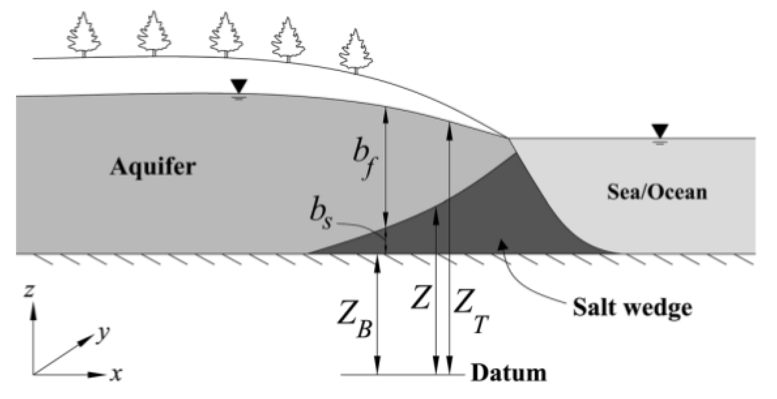
| : water table elevation [m] | : bottom of the aquifer [m] |
| , : hydraulic conductivities [m/day] | , : specific storage coefficients [1/m] |
| , : densities of fresh and saltwater [kg/m] | , : flows [m/day] |
| : porosity of medium [%] | |
| Functions | |
| : freshwater thickness [m] | : saltwater thickness [m] |
| Parameters | ||||||||
|---|---|---|---|---|---|---|---|---|
| Values | 40 | 41 | 1000 | 1025 |
| Scenarios | Sc-1 | Sc-2 | Sc-3 | Sc-4 | Sc-5 | Sc-6 | Sc-7 | Sc-8 | Sc-9 | Sc-10 | Sc-11 |
|---|---|---|---|---|---|---|---|---|---|---|---|
| [m/d] | 0.1 | 0.05 | 0.07 | 0.15 | 0.1 | 0.1 | 0.1 | 0.1 | 0.1 | 0.07 | 0.07 |
| [m] | 150 | 150 | 150 | 150 | 150 | 150 | 200 | 300 | 100 | 150 | 150 |
| [m] | 15 | 15 | 15 | 15 | 0 | 25 | 15 | 15 | 15 | 0 | 25 |
| Wells pumping | |||||
| x [m] | 99,811 | 100,277 | 101,250 | 100,750 | 102,000 |
| y [m] | 384,285 | 383,966 | 375,920 | 374,280 | 375,400 |
| Rate [m/day] | −2918.84 | −2686.99 | −1011.10 | −673.31 | −710.22 |
| Wells pumping | |||||
| x [m] | 99,507.7 | 101,710 | 100,062 | 1,000,000 | |
| y [m] | 375,246 | 374,431 | 372,311 | 374,996 | |
| Rate [m/day] | −1113.03 | −1533.89 | −1402.35 | −1488.54 |
© 2020 by the authors. Licensee MDPI, Basel, Switzerland. This article is an open access article distributed under the terms and conditions of the Creative Commons Attribution (CC BY) license (http://creativecommons.org/licenses/by/4.0/).
Share and Cite
Aharmouch, A.; Amaziane, B.; El Ossmani, M.; Talali, K. A Fully Implicit Finite Volume Scheme for a Seawater Intrusion Problem in Coastal Aquifers. Water 2020, 12, 1639. https://doi.org/10.3390/w12061639
Aharmouch A, Amaziane B, El Ossmani M, Talali K. A Fully Implicit Finite Volume Scheme for a Seawater Intrusion Problem in Coastal Aquifers. Water. 2020; 12(6):1639. https://doi.org/10.3390/w12061639
Chicago/Turabian StyleAharmouch, Abdelkrim, Brahim Amaziane, Mustapha El Ossmani, and Khadija Talali. 2020. "A Fully Implicit Finite Volume Scheme for a Seawater Intrusion Problem in Coastal Aquifers" Water 12, no. 6: 1639. https://doi.org/10.3390/w12061639
APA StyleAharmouch, A., Amaziane, B., El Ossmani, M., & Talali, K. (2020). A Fully Implicit Finite Volume Scheme for a Seawater Intrusion Problem in Coastal Aquifers. Water, 12(6), 1639. https://doi.org/10.3390/w12061639