Article

Tracing the Spatial Distribution of Whole-Lake Exchange of Groundwater and Lake Water in Low-Hydraulic Gradient Systems Using δ18O and Electrical Conductivity and Uncertain End-Member Mixing Analysis

1
Department of Geosciences and Natural Resource Management, University of Copenhagen, Øster Voldgade 10, 1350 K Copenhagen, Denmark
2
Multiconsult Norge AS, 5221 Bergen, Nesttun Hordaland, Norway
3
Freshwater Biology Section, Department of Biology, University of Copenhagen, Universitetsparken 4, 2100 Ø Copenhagen, Denmark
4
Biological Institute, University of Southern Denmark, Campusvej 55, 5230 Odense, Denmark
5
WATEC, Department of Geoscience, Aarhus University, 8000 Aarhus C, Denmark
*
Author to whom correspondence should be addressed.
Water 2020, 12(6), 1608; https://doi.org/10.3390/w12061608
Submission received: 4 May 2020 / Revised: 27 May 2020 / Accepted: 28 May 2020 / Published: 4 June 2020

Abstract

:
δ18O and electrical conductivity (EC) were used successfully to trace the spatial distribution of whole-lake groundwater-lake exchange for a small (four ha) groundwater-fed lake situated in a low relief and low hydraulic gradient area. The method relies on quick sampling of shallow groundwater, direct analysis of EC in the field, and relatively in-expensive analysis of δ18O in the laboratory. Ternary uncertain end-member mixing analysis (precipitation, groundwater, and lake water) quantified the composition of water discharging to and recharging from the lake. The tracer distribution and mixing analysis were in agreement with the interpreted groundwater flow near the lake. The use of only one tracer (either δ18O or EC) gave the same results for the recharge segments, but the discharge segments changed the origin of the water from being groundwater to precipitation controlled. The two tracers complemented each other, especially with different signals in precipitation and groundwater. The uncertain end-members were assessed based on local (groundwater and lake water) and off-site (precipitation) data. The off-site data were found to be useful if it contained representative information on local-site seasonality (uncertainty, variance). Final end-member concentrations could explain the transience of the hydrology at the site (i.e., flooding of the area adjacent to the lake during periods with high precipitation, and variability of the δ18O signal in precipitation). This methodology potentially represents a new option to study groundwater-lake systems. The tracer information collected over only two days is useful by itself for developing the next steps like the quantification of fluxes based on other standard methods (Darcy approach, seepage meters, or temperature). The tracer information can provide quantitative estimation of inputs and outputs by using the mixing analysis.

1. Introduction

Thy National Park in the northwestern part of Denmark houses numerous small (<1 ha) dune lakes, larger kettle hole lakes, and lakes formed by the dissolution of the high-lying Bryozan limestone [1]. The lakes are controlled hydrologically by inputs from precipitation, groundwater, or both. The kettle and dissolution lakes are located within coniferous forests planted to control sand drift. The lakes experience brownification via groundwater input of dissolved organic matter (DOM) [2], which limits light penetration to submerged macrophytes. Management of the forest to both limit input of DOM via groundwater (e.g., by drainage) and, at the same time, securing that enough groundwater still discharges to the lakes is a challenge. Quantification of the spatial input of the invisible groundwater input in relation to forestry and major DOM input at these lakes is therefore essential for keeping good lake water quality.
Estimating the inputs and outputs of groundwater to lakes is a common challenge in hydrological studies. Various field methods for assessing and quantifying groundwater-lake exchange directions and rates have been reviewed earlier [3]. Among the most popular methods to assess groundwater-lake interaction for small lakes is the flow-net analysis or Darcy approach, which relies on measured hydraulic heads in a network of wells, lake stage, and estimates of hydraulic conductivity. Rudnick et al. [4], for example, combined hydraulic heads from a well network around two small German lakes with flow balances to estimate net groundwater discharge (positive/negative). If only the direction of the exchange is needed, then only hydraulic heads around the lake and lake stage are required, preferably as time series. The method can be prone to various types of errors. The most common is how accurate one can measure the differential head between groundwater and the lake. In low-gradient systems like those in Thy National Park, this is especially critical, because even a few centimeters of error can mask the true exchange direction. Labaugh et al. [5] found that it was critical to have wells close enough to the lake to correctly estimate the flow of lake water to groundwater (recharge). Wells located further away from the lake did not capture transpiration-driven lowering of the water table near the lakeshore; hence underestimating outflow from the lake. Many other methods exist and have been used extensively at other Danish lakes (e.g., the temperature-based method [6,7], water balance method [8]), often done in combination with groundwater modeling [7,9,10,11].
Water stable isotopes (δ18O) have been used to assess groundwater-lake interactions [3], typically only for a part of a lakeshore, a lakebed, or with an isotope mass balance for the whole lake, but often not for the spatial distribution of the exchange pattern around the whole lake (whole-lake exchange). The method is becoming increasingly popular due to the conservative properties of water stable isotopes, ease of sampling, and now, relatively easy and in-expensive analysis. Krabbenhoft et al. [12] investigated discharge–recharge patterns on the eastern shoreline of a small lake in Wisconsin, USA, which confirmed the interpreted flow field based on hydraulic heads and lake stage. Furthermore, they were able to derive a stable isotope mass balance to come up with rates of exchange. Petermann et al. [13] used a similar approach with the groundwater end-member based on information from a single groundwater well in the catchment. Rautio and Korkka-Niemi [14] used δ18O in a watershed study of groundwater and river exchange with a large lake in Finland. The groundwater sampling focused on the eastern shoreline in deeper wells and a few mini-piezometers in the lakebed. Kidmose et al. [15,16] assessed groundwater-lake exchanges at two Danish lakes: Lake Hampen, where discharge was observed at two sites and recharge at one site, and Lake Væng, where sampling of the lake bed δ18O revealed only groundwater discharge. Wollschläger et al. [17] sampled time series (three years) of δ18O in the lake water column and deep-screened wells around a small German lake surrounded by gravel pits. In combination with two snapshots of δ18O in shallow groundwater around the lake, they were able to infer groundwater-lake exchange patterns. Karan et al. [9] and Schuster et al. [18] are examples where lakebed profiles of δ18O were used to assess the direction of groundwater-lake exchange and estimate flux rates at a few points in the lakes. Hajati et al. [11] and Krabbenhoft and Webster [19] used the time series of δ18O in groundwater and lakebed at specific locations to investigate flow reversals (i.e., where the direction of exchange between the lake and groundwater changed directions due to seasonal changes in climate).
The use of end-member mixing analysis in connection with use of δ18O is not common. Rautio and Korkka-Niemi [14], and Schuster et al. [18] used a δ18O binary (groundwater and lake water) mixing model to compute lake or groundwater fractions in water sampled from lakebeds. In both studies, the end-member δ18O concentrations were assumed to be known. The use of mixing analysis with uncertain end-members Carrera et al. [20] offers the advantage that end-member concentrations are computed as part of the solution based on initial estimates and an assigned uncertainty. End-member concentrations are never known precisely due to spatio–temporal changes. Müller et al. [21] used δ18O and EC (electrical conductivity) to derive mixing fractions between salt and freshwater in a groundwater-lagoon aquifer. The highest uncertainty was assigned to EC because lagoon salinity was controlled by the operation of a sluice connecting the lagoon to the sea. Transience in hydrology can be detected with a mixing analysis provided there are time series or snapshots of tracer distributions. Jorgensen et al. [22] used a ternary end-member mixing analysis using 87Sr/86Sr and EC to investigate the temporal development of a forced salt water intrusion and extrusion experiment.
The main objectives of this study were as follows. (1) to trace the spatial distribution of whole-lake groundwater-lake exchanges at a small groundwater-controlled lake in Thy National Park, Denmark using δ18O and electrical conductivity (EC) as tracers with a simple and innovative sampling system. Whole-lake exchange is defined here as tracing the exchange along the whole lakeshore. (2) To use uncertain end-member ternary mixing analysis to calculate the composition of subsurface water near the lake bed, evaluate the usefulness of the semi-conservative EC tracer, and use this information to further understand whole-lake exchange and explain how transience in hydrology (precipitation, lake stages, flooding) may have affected subsurface water.

2. Field Site

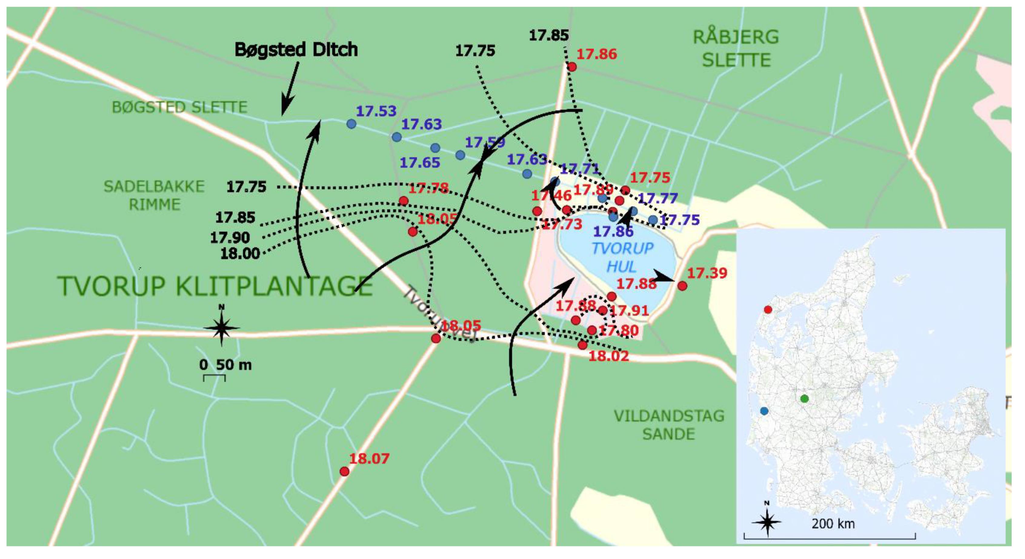
The lake is located within Tvorup Dune Plantation in Thy National Park located along the western coast of Denmark (Figure 1). Lake Tvorup Hul (UTM zone 32, 467420E, 6314252N) is a small lake with an area of 4 ha, a mean depth of 2.4 m, and a maximum depth of 5 m [2]. The lake has no in- or outlets and the water received by the lake originates from precipitation and groundwater. The water residence time (WRT) was estimated to a maximum of two years [2]. The lake is a sinkhole due to dissolution of the high-lying limestone in the area [1]. The area near the lake is flat and at high lake stages, the lake can flood, especially the southern part of the area. A large ditch (Bøgsted) north of the lake is a drainage ditch dewatering the northern area in order to manage the pine tree plantation. The ditch transports water from east to west (Figure 1).
The geology is composed of Aeolian and Marine sand deposits near the surface, underneath is a 2–6 m thick clay layer followed by Bryozoan limestone. The layers slope from east to west; to the east, the sand is roughly 1 m thick with limestone seven meters below surface (mbs). To the west, the sand is roughly 8 m thick. The lake, being on average 2.5 m deep, is therefore in full contact with the top layer of sand, but less near the eastern shoreline due to the thinner sand layer. It is uncertain if the clay layer between the sand and limestone is continuous. There may be areas where there is a hydraulic connection between the sand and limestone and therefore between the limestone and the lake. Soil maps reveal a top layer of sand except at the area east of the lake, described as moraine clay.
Land use is mainly pine tree plantation with drainage by small ditches (especially north of the lake). A flat heath area is located south of the lake. This area is occasionally flooded when the lake stage is high. A ditch running from south of the lake, passing the western side of the lake drains groundwater in the heath area and leads it north of the lake to the Bøgsted Ditch. Drainage was primarily developed to better manage the plantation, and in recent years to divert groundwater with high DOM away from the lake and to Bøgsted Ditch.

3. Methods

3.1. Hydraulic Heads

Twenty-one wells (Figure 1, not all wells are shown) were installed from 2013 to 2017. Galvanized steel pipes with an internal diameter of 1.9 cm and a 9 cm screen at the end were pushed into the sandy subsurface using a pneumatic hammer. All wells were clean-pumped three times the water volume inside the well. Location and top of the well along with stages of the lake and Bøgsted Ditch were measured with a differential global positioning system (DGPS) using a Trimble R8 GPS. Accuracy in vertical direction was 1–2 cm. Hydraulic heads were measured with a Solinst water level meter (accuracy ~1 cm). Uncertainty of the hydraulic head measurements were therefore 2–3 cm. All wells except the well just east of the lake were screened in high-permeable sand (based on slug-tests, data not shown). Final screen depth was from 2 to 10.4 m. Some wells (e.g., TA12, TA13, and TA18) were developed by pushing the pipe to the desired depth, clean-pumping, sampling, and then slug testing, before pushing the pipe further down.

3.2. δ18O and Electrical Conductivity (EC) Sampling and Analysis

δ18O and EC were sampled at 30 locations (February 2016) in shallow groundwater (Figure 2) in the immediate vicinity of the lake [2]. Wells TA12 and TA13 were sampled on 22–23 June 2015 and used for assessing the groundwater end-member compositions. TA18 and surface water in Bøgsted Ditch (BC1-10, Figure 2) were sampled on 22 August 2017 and was later used to confirm that the lake recharged groundwater to the northwest. EC was not measured in the ditch.
Mini-piezometers (diameter of 0.5 centimeter and a 5-centimeter screen) were driven into the subsurface at locations 1–30 by use of a hammer or a small drill to a depth of 1.25 m below the surface. All locations were near the lake, so depth below the surface was almost equal to the depth below the water table. Samples were filtered (0.7 μm nominal pore size Whatman GF/F filters) the same day and stored in a cooler. The samples were analyzed at the Geological Survey of Denmark and Greenland (GEUS) with a PICARRO L2021 using cavity ring-down spectroscopy (CRDS). All values for isotopes are expressed in per-mill (‰) with the δ-notation indicating the deviation from the VSMOW (Vienna Standard Mean Ocean Water):
δ = ( R S a m p l e R V S M O W R V S M O W ) · 1000
RSample and RVSMOW are the 18O/16O isotope concentration ratios of the sample and the VSMOW standard, respectively. EC was measured on-site using a YSI Model 85 conductivity meter (YSI Incorporated, USA). Sampling of the wells and lake were carried out in the same manner.
We had no local data on δ18O and EC in precipitation. δ18O in precipitation (2012–2016) was taken from the study by [23], representing an off-site coastal station at Skjern Enge near Ringkøbing Fjord (http://www.hobecenter.dk/index.php/feltstationer/meadow-site, Figure 2). Skjern Enge and Tvorup Hul are located 16 and 3.5 km from the North Sea, respectively. EC in precipitation (2011–2012) was from an inland field station (http://www.hobecenter.dk/index.php/feltstationer/voulund, Figure 2, 66 km from the coast, [24]).

3.3. End-Member Mixing Analysis

The MIX code by [20] was used to compute mixing fractions and end-member concentrations. Mixing analysis is often performed assuming the end-members are perfectly known. The MIX code allows for uncertain end-member concentrations, where a variance can be assigned to the initially assumed concentrations. The MIX code uses a maximum likelihood approach to compute mixing fractions and improved estimates of end-member concentrations. A guess for initial mixing fractions and end-member concentrations is required. In this case, single (either δ18O or EC) or dual (both) tracers were used in the analysis. Uncertainty can be due to: (1) temporal changes in δ18O or EC in end-members; (2) end-member tracers were not measured exactly at the study site; or (3) end-members approximated in some other manner. Each sample from the 1–30 sampling locations was also assigned an uncertainty related to the accuracy by which the samples can be analyzed in the field (EC) or the laboratory (δ18O). The mixing analysis requires that the tracers are conservative, which is not necessarily the case for EC, see Section 4.4.

4. Results

4.1. Groundwater Flow System

Groundwater flows from the south and north toward the lake (Figure 1). Bøgsted Ditch affects the groundwater flow pattern by capturing shallow groundwater flowing toward the lake from the north and diverting some of the groundwater originating from the south to the ditch. In addition, it causes the lake to be drained through its northern shoreline. The lake recharges groundwater to the east. The differences between the water level in the lake (17.86 m) and the groundwater table are about 10 cm or less near the lake (50–100 m). Considering the accuracy of the measurements (2–3 cm), the iso-potential map and flow patterns should be interpreted with caution. For example, in the relatively flat area just south of the lake, hydraulic heads ranged from 17.80–18.03 m (even one well showing a gradient from the lake to groundwater). The time of measurement plays a big role in the interpretation of the iso-potential map. Time series of hydraulic heads in TA12 and TA13, and lake stage (for locations, see Figure 2) showed differences up to 0.4 m over the year (Figure 3). Hydraulic heads in TA13 were for the most part 0.3–0.4 m higher than the lake level. However, there were also periods where there was a reversed, but small gradient (−0.08 m in November 2015). Hydraulic heads in TA12 were consistently higher than the lake levels, but it is not clear if groundwater near TA12 flows to the lake or more westerly toward the ditch (Figure 1).

4.2. δ18O and EC Tracers in Groundwater and Lake

Lake Tvorup Hul showed seasonal oscillations in EC and δ18O (Figure 4). The lake water residence time (ca. 2 years) is sufficiently long to allow for some isotopic fractionation due to evaporation, leading to an enriched concentration of −4.1 to −5.2‰. Although data are scarce, a seasonal amplitude of 0.5‰ can be determined, much lower than in precipitation. EC was relatively constant with values ranging from 100–160 μS/cm. Note that δ18O decreased by 1‰ from November 2014 to March 2015 and then increased by the same amount from March 2015 to June 2015. Several other lakes surveyed in the area showed the same pattern. No obvious explanation to this could be found in the weather data (precipitation, number of hours with sunshine), which were close to normal from 2006–2015.
Profiles of EC and δ18O in groundwater were used as an indication of flow paths and source areas of recharge (Figure 5). EC was in the range 200–250 μS/cm at depths greater than 6 mbs. The clay layer could thus affect EC at these depths. However, EC values from 50 other wells in the area (average screen depth of 3 m, 1–2 m below the water table, and, thus not affected by the clay layer) resulted in an average of 262 μS/cm. The two profiles were very different down to 6 mbs with TA12 showing a high EC peak at 3 mbs. This is likely the result of rainfall infiltrating the forest soils and then diluted with lower EC groundwater at greater depths. TA18 showed values near the lake EC, indicating that lake water recharges groundwater to the northwest. This is also clear from the δ18O profile in TA18 having values close to those measured in the lake (Figure 5). At depths greater than 7 mbs, δ18O concentrations decreased, which might be the result of the lake having a maximum depth of 5 m, confining the δ18O-plume to the upper 0–7 mbs. The δ18O profiles in TA12 and TA13 are clearly distinct from that of TA18 and resemble the average δ18O in precipitation.

4.3. δ18O and EC Tracers in Shallow Groundwater (Sampling Locations 1–30)

The δ18O and EC concentrations in the 30 sampling locations around the lake and of two lake samples showed an uneven distribution (Figure 6). Recalling that the average δ18O in precipitation and groundwater at some depth was −8‰ made it possible to evaluate qualitatively, where the discharge of groundwater takes place. This seems to take place across half of the southern shoreline (sampling locations 2–7). The two lake samples showed an enriched signal (-4.6), which makes it possible to trace lake water recharging groundwater along most of the western and northern shorelines (locations 16–29). This agrees with the interpreted iso-potential map (Figure 1) and the samples from Bøgsted Ditch (Figure 7). The samples from the ditch were not from the sediment bed, but grab samples of the water in the ditch. Figure 6A and Figure 7 show a δ18O lake water plume originating from the northwestern shoreline feeding into the ditch, here mixing with groundwater from the north draining to the ditch. Note that the upstream part of the ditch is affected more by recharge from the lake than the downstream part. The results from the eastern shoreline do not show a clear discharge or recharge signal. The EC samples cannot trace the same discharge–recharge pattern, although the samples along most of the northern shoreline best reflected the low EC measured in the lake (Figure 4). Samples 9 and 11 (400–800 μS/cm) were very different from the rest and may reflect groundwater coming from the clay layer or the limestone.

4.4. Mixing Analysis

Three end-members were chosen: precipitation, groundwater, and lake water. In reality, groundwater that discharges to the lake comes from precipitation (or recharge). A sample of shallow groundwater discharging to the lake will be a mixture of old upward flow of groundwater from the catchment carrying the average isotopic concentration of precipitation, and new groundwater from recent infiltration carrying the isotopic signature of recent precipitation (or recharge). We chose to distinguish between the two in order to better differentiate between the sources of a sample on the discharge side of the lake. EC is not necessarily a conservative tracer as required by the mixing analysis. However, it was our hypothesis that EC would work as a tracer: (a) on the recharge side, because the flow distances from the lakeshore to the sampling locations were only a few meters, so that changes in EC would be small; and (b) the changes in EC in groundwater on the discharge side due to biogeochemical changes would be relatively small compared to the contrast in EC between groundwater, precipitation, and lake water.
The data presented in Section 3.1 and Section 3.2 (Table 1) were used to assess the initial end-member concentrations for δ18O and EC and associated uncertainty. Both EC and δ18O concentrations were evaluated based on concentrations from a depth greater than 6 mbs (Figure 5). The deeper groundwater was assumed to flow horizontally to the lake and then vertically upward near the sampling locations. δ18O in precipitation at Skjern Enge had a mean, maximum, and minimum of −8.0‰, −5.1‰, and −12.2‰, respectively. The seasonal amplitude was ~3.5‰ [23]. Three very high EC concentrations in precipitation (108–211 μS/cm, [24]) were not included (the source of these high concentrations are not known).
There are differences in EC concentrations between precipitation, groundwater, and lake water (Table 1). For δ18O, the main difference was between lake water and that of groundwater or precipitation. The uncertainty in δ18O in precipitation was higher (σ = 1.57‰) than for groundwater and lake water due to the seasonality of δ18O in precipitation. This seasonality or uncertainty was significantly damped once in groundwater or in the lake.
The MIX code can also handle uncertainty in sample concentrations. The uncertainty or average standard deviation of the laboratory analysis of δ18O samples was 0.08‰. For EC, a 10% uncertainty due to instrumental error on the maximum mean EC was used, in this case, a standard deviation of 20 μS/cm.

4.4.1. Mixing Analysis Based on Dual Tracers (EC + δ18O)

The MIX code gave final estimates of the end-member concentrations (Table 2 and Figure 8). The initial and final estimated EC end-member concentrations for precipitation and lake water were not changed much. For groundwater, the concentration increased from 219 μS/cm to 292 μS/cm. Precipitation decreased from 37 μS/cm to 25 μS/cm, which was unexpected as the lake is located closer to the coast than the inland station used to evaluate EC in precipitation. The δ18O for precipitation was estimated to a lower more depleted concentration (from −7.95‰ to −10.71‰), while that of the lake water was found to be more enriched (from −4.48‰ to −3.38‰). Groundwater remained approximately the same. The initial estimates based on local and off-site end-member concentrations were far from bracketing the observed values at the sampling stations, showing the need for adjusting the end-member concentrations (Figure 8). However, with the assigned uncertainty, the MIX model could estimate new end-member concentrations that bracketed all observations except three.
The mixing analysis estimates fractions of precipitation, groundwater, and lake water for each sampling location. The sum of the three fractions equaled one. Subsurface water at the southern shoreline was mostly composed of groundwater (samples 30 and 1–7 with fractions of 0.4–0.6) and some lake water (0–0.33) (Figure 9). Precipitation (Figure 10) will then be the remaining fraction. Likewise, subsurface water at the northern and western shoreline was mostly composed of lake water (~0.7 and higher; samples 16–29, Figure 9B) and some groundwater (0–0.2, Figure 9A). The precipitation fraction was close to 0.1 (Figure 10). Figure 9 shows where discharge and recharge were estimated to occur based on this analysis for 27 locations. If the dominant fraction was groundwater or lake water, it was classified as a discharge or recharge segment, respectively.

4.4.2. Mixing Analysis Based on EC Only and δ18O Only

To understand the effect of using more than one tracer on the analysis and evaluate the cost/benefit of combining both tracers, similar calculations were done using either EC or δ18O. The end-member EC concentration remained approximately the same as the initial value (Table 2). A more depleted value for precipitation was calculated, although less depleted than in the dual tracer approach. Likewise, lake water had an enriched value in δ18O and more so compared to the dual tracer approach. A slightly more enriched value in δ18O was also computed for groundwater.
The comparison using three combinations of tracers EC and δ18O, only δ18O, and only EC showed significant differences between estimated fractions for groundwater, lake water, and precipitation. The choice of using a single tracer, and which one, or a dual tracer has a clear impact on the calculated fractions. Using either EC or δ18O alone cannot predict fractions, which are in general agreement with the iso-potential map and the areas where discharge and recharge are identified do not match. For the groundwater fractions (Figure 11a), using only EC as a tracer, the mixing analysis estimated nearly the same fractions at the southern shoreline, where discharge was expected. However, on the northern and western shorelines, the groundwater fractions were much higher than calculated using the dual-tracer approach. Using δ18O alone gave a completely different interpretation on the southern lakeshore with very small groundwater fractions. Instead, samples were estimated to be composed primarily of precipitation with fractions >0.55 (Figure 11c). In contrast, using δ18O alone, the composition for most samples along the northern and western shoreline was predicted to be composed primarily of lake water.

5. Discussion

Lake Tvorup Hul is located in a groundwater system with low hydraulic gradients. To use measured hydraulic heads from a few wells to assess the interaction between groundwater and the lake can therefore be challenging, because small measurement errors, or short-term transience in the heads and lake stage, can mask the interpretation.
Tracers can be a valuable alternative that, with a minimum of effort, can give a clear representation of groundwater–lake interactions. Tracers reflect longer-term flow processes and are thus less affected by short-term changes in precipitation. δ18O is especially useful; it is easy to sample and analyze, and has distinct and relatively constant concentrations in deeper groundwater and lake water relative to precipitation. The seasonality of δ18O in precipitation is damped in groundwater (due to mixing) and in the lake (due to fractionation). The δ
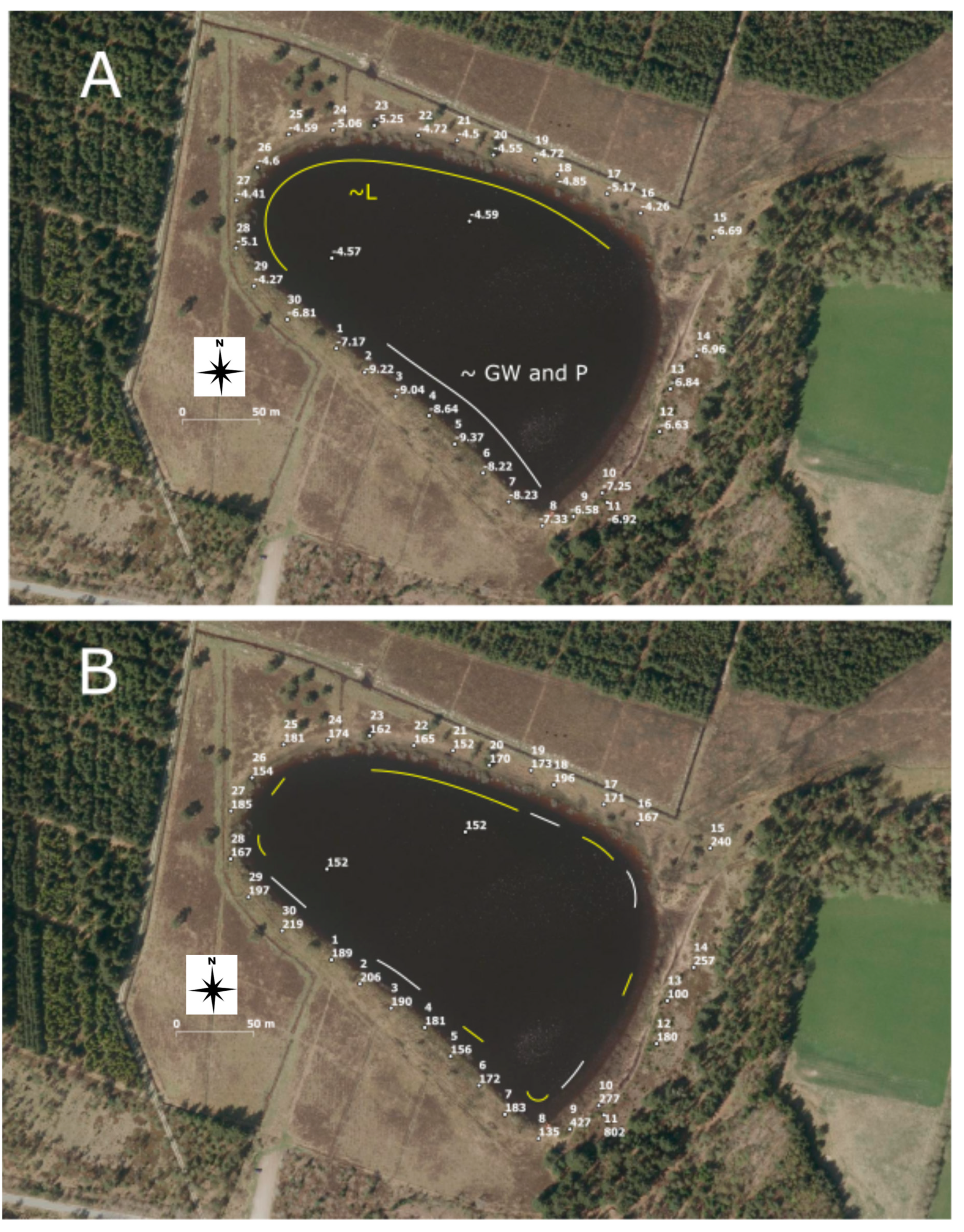
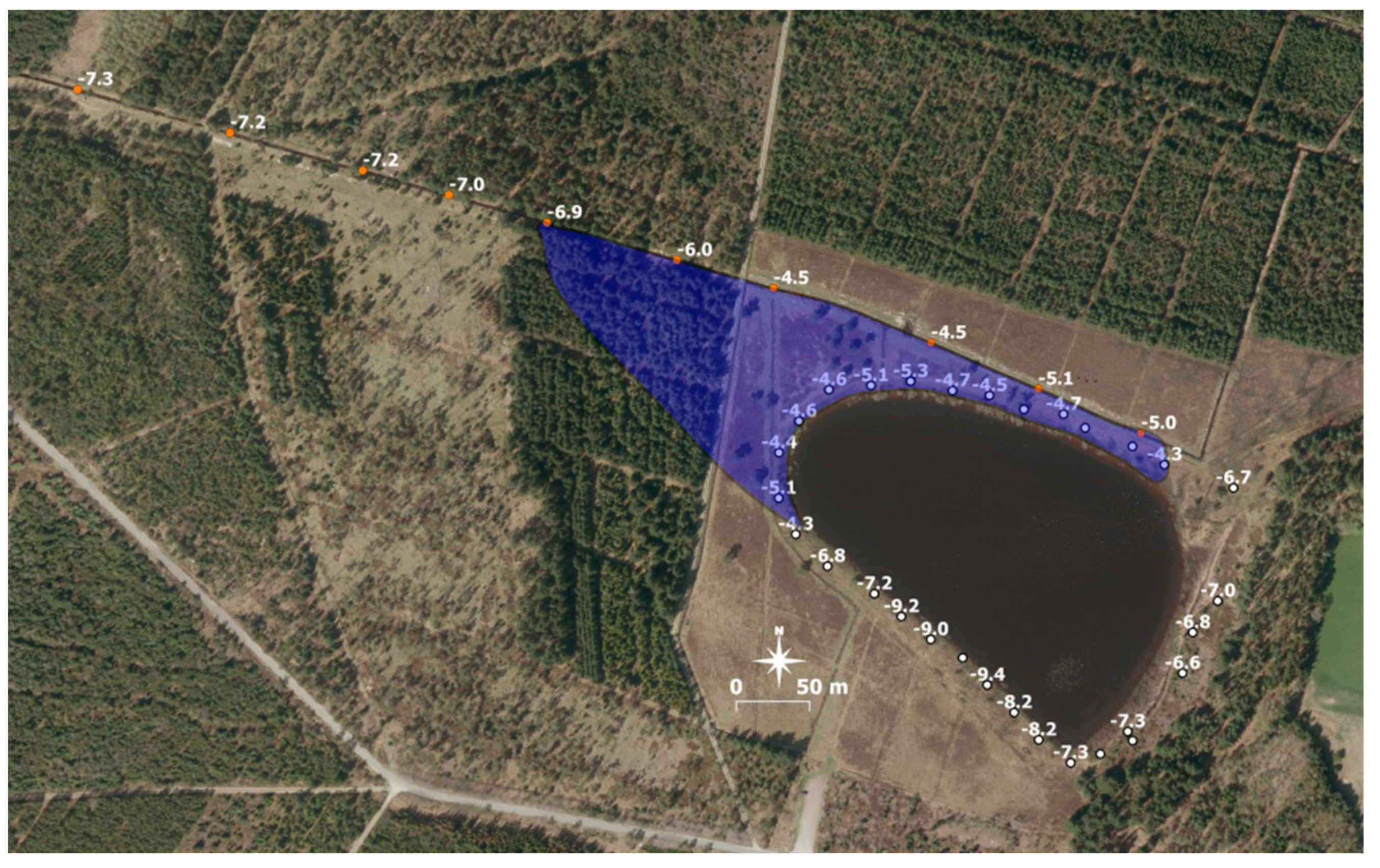
18O concentrations in shallow groundwater around the lake (Figure 6A) make it relatively easy to define the discharge and recharge zones for the whole lake. Other studies have obtained the same type of results, but typically only for parts of a lake [12,14,15]. The research by Kidmose et al. and Wollschläger et al. [16,17] are examples of whole-lake δ
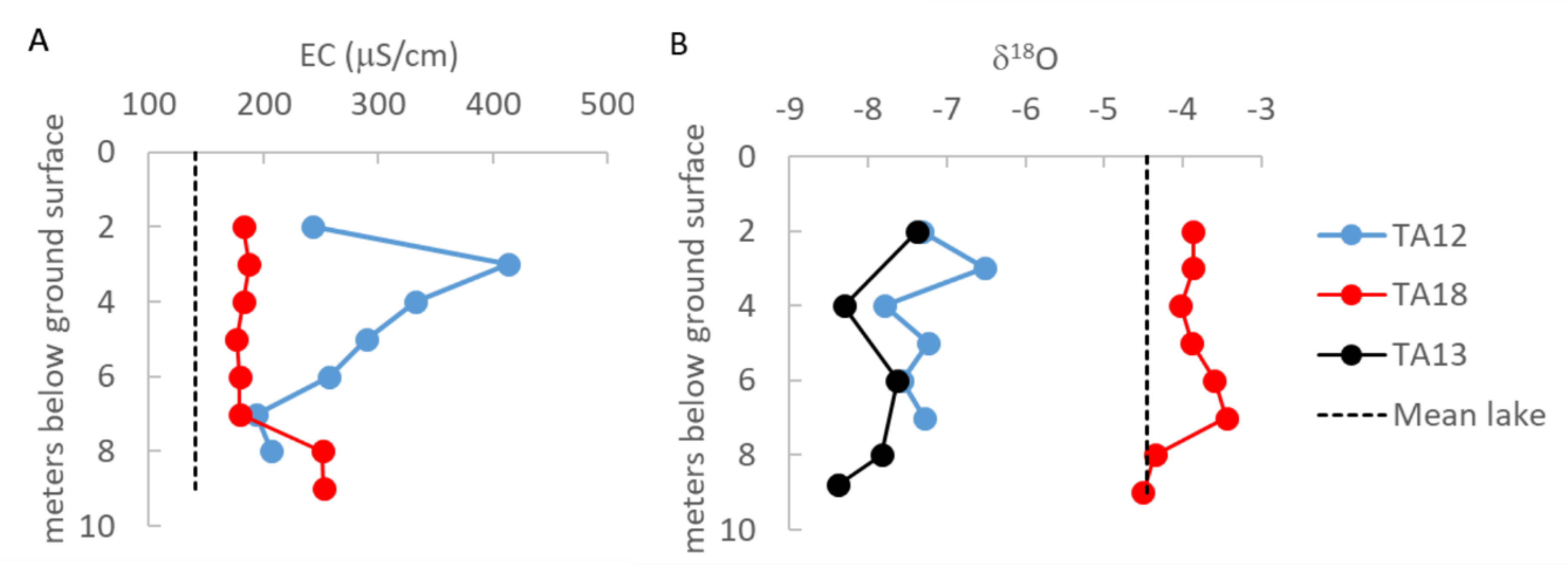
18O studies, but using a much lower sampling intensity. EC is easy and frequently measured in the field, but is not as straightforward to use, which is partly because it is a semi-conservative tracer. Biogeochemical processes in soils, groundwater, and the lake may affect EC. However, it was possible to identify lake segments with the recharge of groundwater along the northern shoreline (Figure 6B). EC increased only slightly (from around 150–160 μS/cm in the lake to 152–171 μS/cm) with flow of the tracer from the lake and to the sampling locations in recharge segments a few meters away. For both tracers, recharge of groundwater from the lake was best identified because of the distinct lake δ18O and EC signals (Figure 8).
The end-member mixing analysis is a quantitative approach and assigns mixing fractions to a sample. In our case, we chose three main end-members: precipitation, groundwater, and lake water. This required information on end-member concentrations and, if using the MIX code, an estimate of the uncertainty of end-member concentrations. The mixing analysis for the dual tracer approach is in good agreement with the qualitative interpretation from the δ
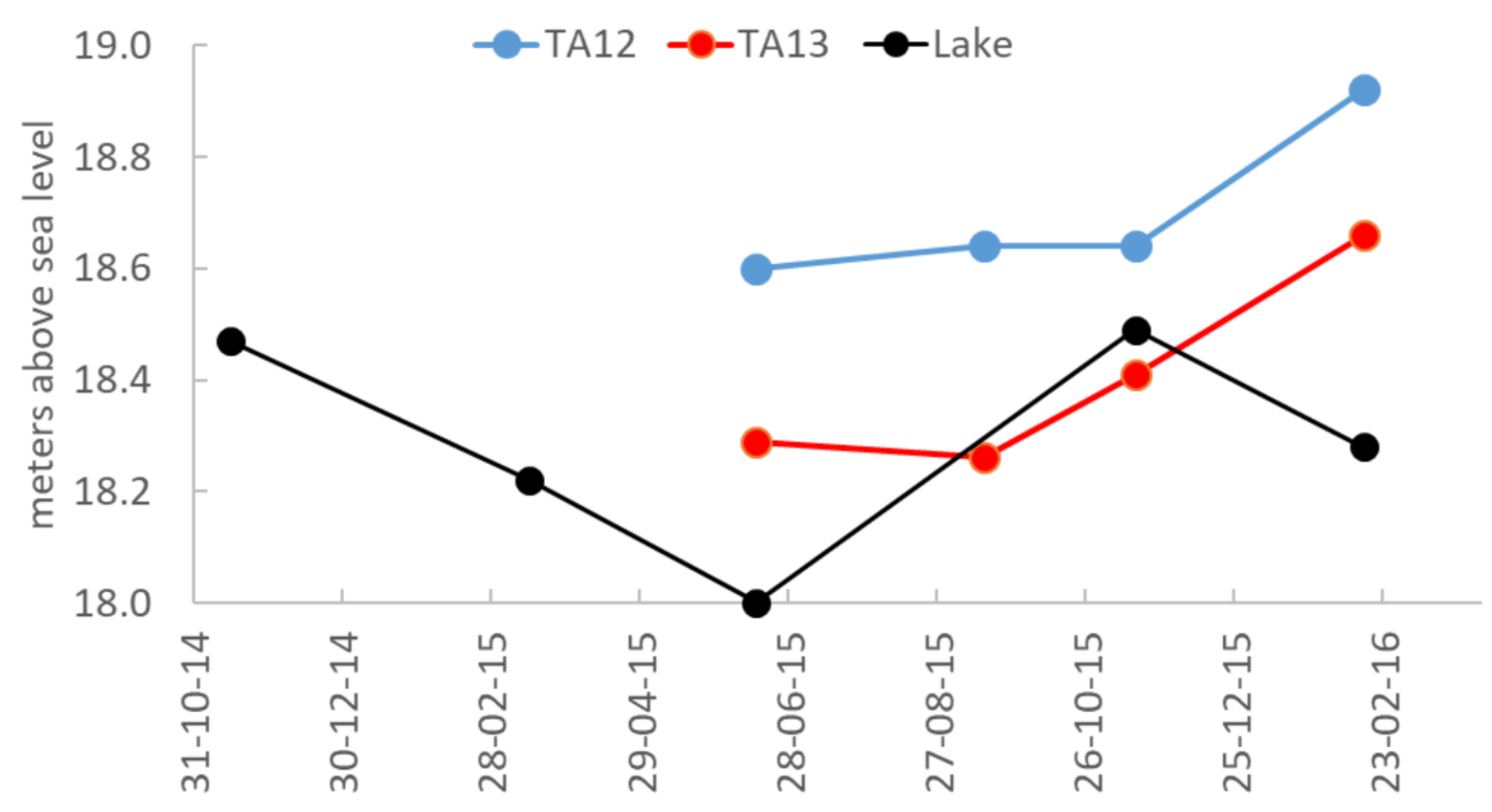
18O samples and the interpreted groundwater flow. The mixing analysis can give additional insights into temporal changes in groundwater–lake interactions in a low-relief area like that surrounding Lake Tvorup Hul. For example, high groundwater fractions along the southern shoreline, relatively high fractions of precipitation, and samples with fractions of lake water (0.1–0.15) were calculated along a continuous segment (locations 30 and 1–7, Figure 10). In extreme cases, the lake stage can increase by up to 0.5 m (Figure 3). Lake water in these samples could be due to flooding of the area south of the lake. Depending on the duration of the flooding, lake water may infiltrate to the shallow groundwater and mix with groundwater and precipitation. We interpreted the co-existence of high fractions of groundwater and precipitation at the southern shoreline (Figure 10) as deeper groundwater flowing upwards toward the lake shore and mixing with vertically downward infiltrating precipitation. The final end-member δ18O precipitation concentrations were more depleted in cases when EC/δ18O or δ18O alone were used in the mixing analysis (Table 2, Figure 8). All samples were collected at a depth of 1.25 m below surface in February 2016 (essentially the same as the depth below the water table). Recharge estimate in this region is 0.5 m/year, and with a porosity of 0.3, this gives a vertical downward pore water velocity of 1.5 m/year. In other words, the fraction of precipitation in samples 30 and 1–7 could be a winter slug of precipitation from a year before sampling. The precipitation data (collected off-site) showed many examples of δ18O concentrations around −10‰ in the winter months, so it is reasonable to assume that similar depleted values were present in local precipitation. The greatest uncertainty in any end-member concentrations was in δ18O in precipitation. The off-site data may therefore not accurately predict the initial local end-member concentration, but the observed off-site seasonal variability can be used to estimate the end-member concentration more precisely at the time of sampling. The reason we do not see the same fraction of precipitation on the recharge side of the lake could be due to the much smaller infiltration area between the lake and Bøgsted Ditch. If we had attempted to use a binary end-member mixing analysis with groundwater and lake water (excluding precipitation), then we would expect the estimated end-member concentration of groundwater to be much more depleted compared to the average composition of precipitation. We would then have arrived at the same conclusion, that a sample on the discharge side was a mixture of older and younger groundwater, but without the possibility of estimating the two fractions. Otherwise, we would not have been able to fit the depleted values along the discharge segment of the lake.
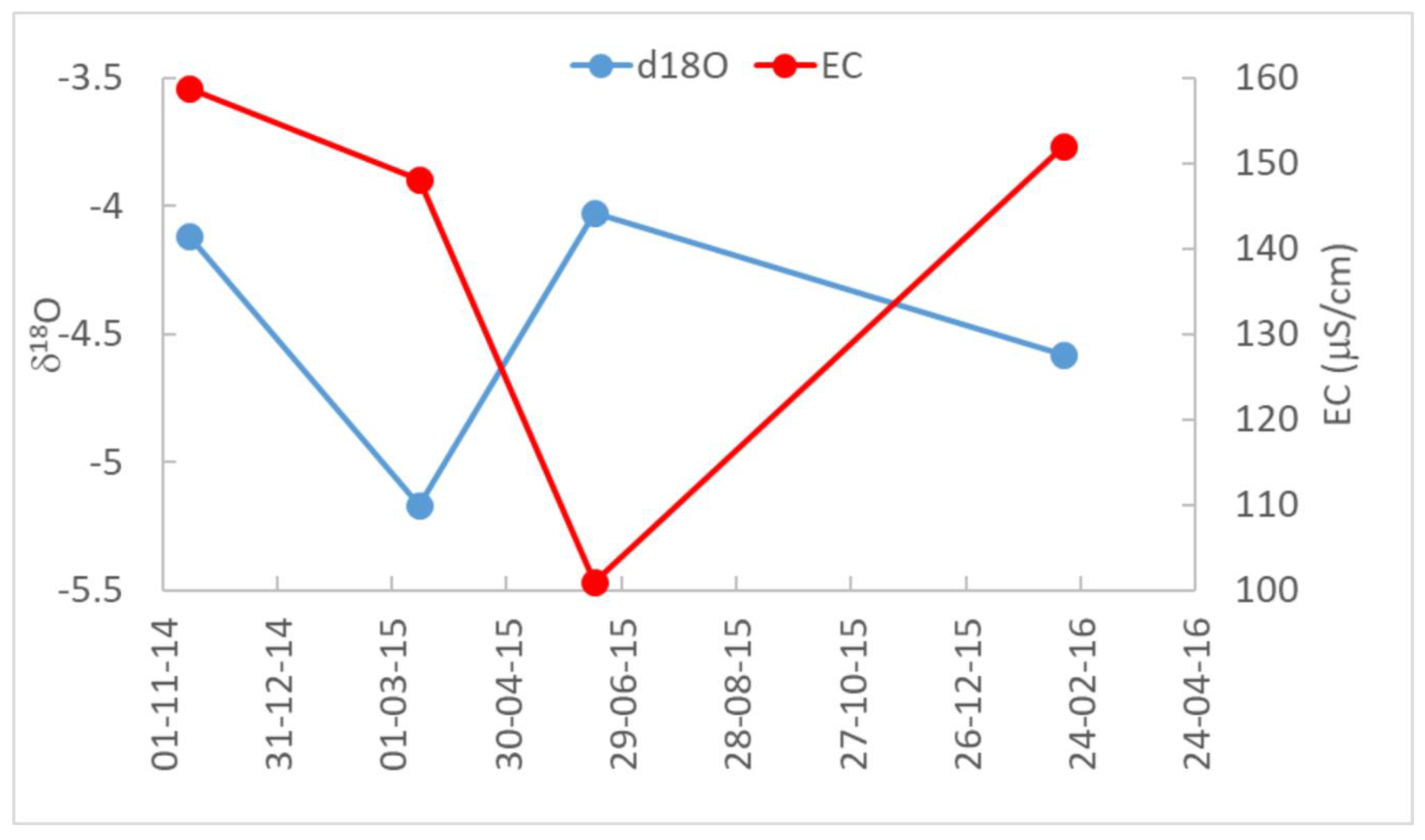
The final lake δ18O end-member was more enriched than what was originally estimated. This may be explained by one outlier in the lake data with a less enriched value of −5.17‰ (1 March 2015), which greatly influenced the initial choice of end-member concentration. If this measurement had been excluded, the initial value would have been more enriched and closer to the final end-member concentration.
EC end-member concentration in groundwater increased by 25%. We cannot rule out that this change is because EC is not a fully conservative tracer. What was more surprising was that EC in precipitation was further decreased compared to the data from the inland station. One would expect a higher end-member concentration due to the proximity of the lake to the ocean. This was due to sample 13 (from the eastern shoreline, Figure 8) with an EC of 100 μS/cm lying exactly on the mixing line between precipitation and lake water. Neighboring samples 12 and 14 had approximately the same δ18O concentrations, but much higher EC concentrations closer to that of groundwater (180–257 μS/cm). If sample 13 had been excluded from the analysis, then the EC in precipitation could have been higher.
These uncertainties also had an implication when using δ18O or EC alone as a tracer in the end-member mixing analysis. Using δ18O concentrations alone could not distinguish between precipitation and groundwater discharging along the southern shoreline. This is likely a result of the initial end-member concentrations of groundwater and precipitation, being almost identical (Table 2). In fact, precipitation was the major fraction along this segment of the lake (Figure 11a,c). Adding EC helped the mixing analysis because of the distinct difference between groundwater and precipitation (Table 2). Along the same line, both tracers were able to estimate the fractions on the northwestern lake segment because of the similarity in lake water and groundwater composition.
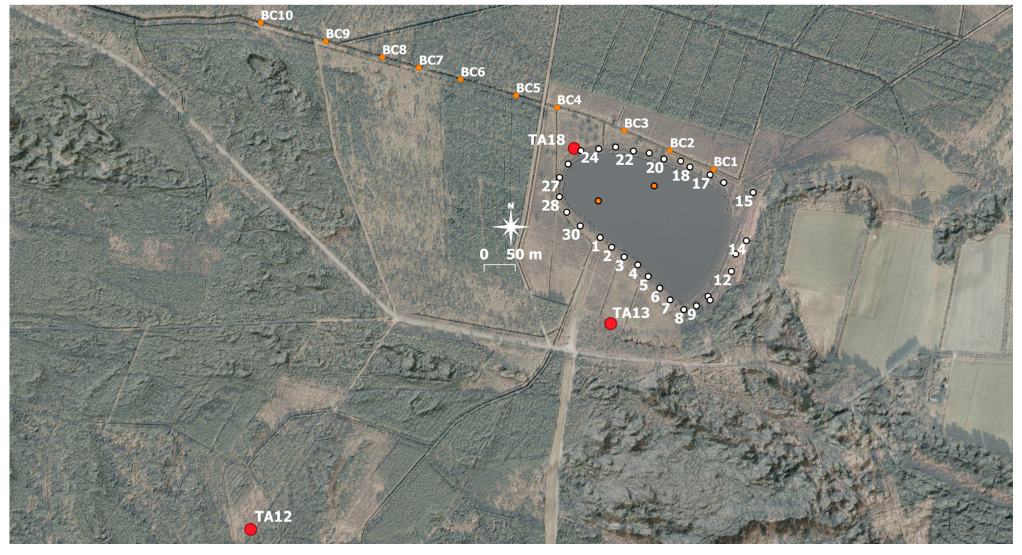
The effort of collecting these data amounted to roughly two days of field work for a small lake like Tvorup Hul. The ease with which the field work was carried out was partly due to the sandy material in the top making installation of mini-piezometers, clean pumping, and sampling swift. EC was measured in situ so already during field work, one can get an indication of the directions of the exchange of water between groundwater and the lake. This can guide the choice of spacing between sampling locations. The interpretation of groundwater–lake interactions is then readily carried out, which for Lake Tvorup Hul resulted in zones of groundwater discharge from the south, and recharge to groundwater to the north (and then the ditch) and west. At the eastern lakeshore, results were not conclusive, showing both discharge and recharge. There are several reasons for this. First, the lake is not hydraulically well connected to the sand layer, the layer being only ~1 m thick with clay below. Second, we had a well a few hundred meters to the northeast of the lake, screened in limestone at 4.6 mbgs. The well was destroyed by forest machinery, but a few head measurements in the fall of 2015 gave values of 14.2 m, significantly below the lake stage, thus indicating outflow or recharge. Third, it can be seen from Figure 2 that a small ridge appear just east of the lake, so it is possible that a small groundwater divide could form just east of the lake with occasional discharge to the lake.
Tracers and mixing analysis can be helpful as a first-step in guiding how to establish a monitoring network for better understanding dynamic groundwater–lake interactions. The use of end-member mixing analysis proved valuable in understanding the ternary mixing of precipitation, groundwater, and lake water around the lake and how seasonality in lake stage, flooding, and slugs of precipitation infiltrating the soils may have influenced mixing fractions. This requires knowledge of end-member concentrations, which may not always be available at the desired precision. The MIX code can partly deal with this by allowing for uncertain end-members. Local (lake and groundwater in this case) and off-site (precipitation) information was here used to assess uncertainty, but still, the results were consistent with the rest of the observations done in the field site, indicating that this methodology could be easily exported to study groundwater–lake interactions in other regions with different access to data.

6. Conclusions

This study used δ18O and electrical conductivity (EC) to trace the spatial distribution of whole-lake groundwater-lake exchange and ternary uncertain end-member mixing analysis to quantify the composition of water discharging to or recharging from the lake. The study was carried out at a small groundwater-fed lake with low relief and low hydraulic gradients.
Use of both tracers could accurately depict the spatial pattern of exchange with discharge along the southern lakeshore and recharge along the western and northwestern lakeshore. Exchange along the eastern lakeshore was more uncertain, likely due to poor contact with the sandy aquifer. The tracer results were in good agreement with the interpreted groundwater flow based on hydraulic head data and lake stage.
Use of one tracer alone did not show the same clear exchange pattern along the whole lakeshore. Recharge was still predicted in the same locations, which was caused by a clear enriched signal in δ18O and low EC values in lake water. Where discharge occurred was not as clear, because δ18O in groundwater and precipitation were quite similar in this area. Although EC is a semi-conservative tracer, it proved helpful to assess where the groundwater was discharging, because of the clear difference in EC of the three end-members: groundwater, lake water, and precipitation.
The combination of using several tracers and uncertain end-member mixing analysis is a powerful diagnostic tool in the early phases of an investigation of groundwater–lake interactions. The ternary mixing analysis with uncertain end-members corroborated the qualitative interpretation based on the tracers alone and provided new insights about how transience in hydrology (precipitation, changes in lake stages flooding of an area next to the lake) affected the composition of water discharging to the lake or recharged from the lake. An outcome of the mixing analysis is new estimated end-member concentrations. This was especially useful on the discharge side of the lake, where the use of the two tracers estimated that the water was mainly a mixture of precipitation (~1 year old) and deep groundwater, and less so of lake water (from occasional flooding at high lake stages). This study also demonstrates that the use of off-site precipitation end-member information to predict local conditions is possible. It is important, though, that the off-site data represent the uncertainty in end-member concentrations (seasonality, variance).

Author Contributions

Conceptualization, P.E., E.K., T.K., I.S.S., and C.D.; Methodology, P.E., T.K., E.K., I.S.S., and C.D.; Formal analysis, T.K., P.E. and C.D.; Investigation, T.K., E.K., I.S.S., and M.S.; Writing—original draft preparation, T.K., P.E. and C.D.; Writing—review and editing, T.K., P.E., C.D., E.K., I.S.S., and M.S. All authors have read and agreed to the published version of the manuscript.

Funding

The work was funded by the Villum Foundation through a grant to CLEAR—a Villum Center of Excellence 2006–2010.

Acknowledgments

Henrik Schjødt Kristensen from The Danish Nature Agency in Thy kindly granted access to the site. Many geology students following the hydrogeological field course contributed greatly to the collection of data. We thank Jörg Lewandowski and an anonymous reviewer for the excellent feedback that greatly improved the paper.

Conflicts of Interest

The authors declare no conflicts of interest.

References

  1. Granat, H.J.; Secher, K. Geologi og Jordbund—Thy Statsskovsdistrikt (In Danish: Geology and Soils—Thy Fforest); Skov- og Naturstyrelsen og Danmarks og Grønlands Geologiske Undersøgelse: Copenhagen, Denmark, 2006; p. 83. Available online: https://naturstyrelsen.dk/media/nst/Attachments/Thy_geologi_2006low.pdf (accessed on 31 May 2020).
  2. Kristensen, E.; Madsen-Østerbye, M.; Massicotte, P.; Pedersen, O.; Markager, S.; Kragh, T. Catchment tracers reveal discharge, recharge and sources of groundwater-borne pollutants in a novel lake modelling approach. Biogeosciences 2018, 15, 1203–1216. [Google Scholar] [CrossRef] [Green Version]
  3. Rosenberry, D.O.; Lewandowski, J.; Meinikmann, K.; Nützmann, G. Groundwater—The disregarded component in lake water and nutrient budgets. Part 1: Effects of groundwater on hydrology. Hydrol. Process. 2015. [Google Scholar] [CrossRef]
  4. Rudnick, S.; Lewandowski, J.; Nützmann, G. Investigating Groundwater-Lake Interactions by Hydraulic Heads and a Water Balance. Ground Water 2014. [Google Scholar] [CrossRef] [PubMed]
  5. LaBaugh, J.W.; Rosenberry, D.O.; Mushet, D.M.; Neff, B.P.; Nelsond, N.H.; Euliss, R.D., Jr. Long-term changes in pond permanence, size, and salinity in Prairie Pothole Region wetlands: The role of groundwater-pond interaction. J. Hydrol. Reg. Stud. 2018, 17, 1–23. [Google Scholar] [CrossRef]
  6. Sebok, E.; Duque, C.; Kazmierczak, J.; Engesgaard, P.; Nilsson, B.; Karan, S.; Frandsen, M. High-resolution distributed temperature sensing to detect seasonal groundwater discharge into Lake Væng, Denmark. Water Resour. Res. 2013, 49, 1–14. [Google Scholar] [CrossRef]
  7. Kazmierczak, J.; Müller, S.; Nilsson, B.; Postma, D.; Czekaj, J.; Sebok, E.; Jessen, S.; Karan, S.; Jensen, C.S.; Edelvang, K.; et al. Groundwater flow and heterogeneous discharge into a seepage lake: Combined use of physical methods and hydrochemical tracers. Water Resour. Res. 2016, 52. [Google Scholar] [CrossRef]
  8. Ommen, D.A.O.; Kidmose, J.; Karan, S.; Flindt, M.R.; Engesgaard, P.; Nilsson, B.; Andersen, F.Ø. Importance of groundwater and macrophytes for the nutrient balance at oligotrophic Lake Hampen, Denmark. Ecohydrology 2012, 5, 286–296. [Google Scholar] [CrossRef]
  9. Karan, S.; Kidmose, J.; Engesgaard, P.; Nilsson, B.; Frandsen, M.; Ommen, D.A.O.; Flindt, M.R.; Andersen, F.Ø; Pedersen, O. Role of Groundwater-Lake Interface in Controlling Seepage of Water and Nitrate. J. Hydrol. 2014. [Google Scholar] [CrossRef]
  10. Kidmose, J.; Engesgaard, P.; Ommen, D.A.O.; Nilsson, B.; Flindt, M.R.; Andersen, F.Ø. The role of groundwater on lake restoration: Simulation of nutrient (N) seepage. Ground Water 2015. [Google Scholar] [CrossRef]
  11. Hajati, M.-C.; Frandsen, M.; Pedersen, O.; Nilsson, B.; Engesgaard, P. Flow reversals in groundwater-lake interactions: A natural tracer study using δ18O. Limnologica 2018, 68, 26–35. [Google Scholar] [CrossRef]
  12. Krabbenhoft, D.P.; Bowser, C.J.; Anderson, M.P.; Valley, J.W. Estimating groundwater exchange with lakes 1. The stable isotope mass balance method. Water Resour. Res. 1990, 26, 2445–2453. [Google Scholar] [CrossRef]
  13. Petermann, E.; Gibson, J.J.; Knöller, K.; Pannier, T.; Weiss, H.; Schubert, M. Determination of groundwater discharge rates and water residence time of groundwater-fed lakes by stable isotopes of water (18O, 2H) and radon (222Rn) mass balances. Hydrol. Process. 2018, 32, 805–816. [Google Scholar] [CrossRef]
  14. Rautio, A.; Korkka-Niemi, K. Chemical and isotopic tracers indicating groundwater/surface-water interaction within a boreal lake catchment in Finland. Hydrogeology 2015, 23, 687–705. [Google Scholar] [CrossRef]
  15. Kidmose, J.; Engesgaard, P.; Nilsson, B.; Laier, T.; Looms, M.C. Spatial distribution of seepage at a flow through lake: Lake Hampen, Western Denmark. Vadose Zone J. 2011, 10, 110–124. [Google Scholar] [CrossRef]
  16. Kidmose, J.; Nilsson, B.; Engesgaard, P.; Frandsen, M.; Karan, S.; Landkildehus, F.; Søndergaard, M.; Jeppesen, E. Focused groundwater discharge of phosphorus to a eutrophic seepage lake: Implications for lake ecological state and restoration. Hydrogeol. J. 2013. [Google Scholar] [CrossRef]
  17. Wollschläger, U.; Ilmberger, J.; Isenbeck-Schröter, M.; Kreuzer, A.M.; von Rohden, C.; Roth, K.; Schäfer, W. Coupling of groundwater and surface water at Lake Willersinnweiher: Groundwater modeling and tracer studies. Aquat. Sci. 2007, 69, 138–152. [Google Scholar] [CrossRef]
  18. Schuster, P.F.; Reddy, M.M.; LaBaugh, J.W.; Parkhurst, R.S.; Rosenberry, D.O.; Winter, T.C.; Antweiler, R.C.; Dean, W.E. Characterization of lake water and ground water movement in the littoral zone of Williams Lake, a closed-basin lake in north central Minnesota. Hydrol. Process. 2003, 17, 823–838. [Google Scholar] [CrossRef]
  19. Krabbenhoft, D.P.; Webster, K.E. Transient hydrogeological controls on the chemistry of a seepage lake. Water Resour. Res. 1995, 31, 2295–2305. [Google Scholar] [CrossRef]
  20. Carrera, J.; Vázquez-Suñé, E.; Castillo, O.; Sánchez-Villa, X. A methodology to compute mixing ratios with uncertain endmembers. Water Resour. Res. 2004, 40, W12101. [Google Scholar] [CrossRef] [Green Version]
  21. Müller, S.; Jessen, S.; Duque, C.; Sebok, E.; Neilson, B.; Engesgaard, P. Assessing seasonal flow dynamics at a lagoon saltwater–freshwater interface using a dual tracer approach. J. Hydrol. Reg. Stud. 2018, 17, 24–35. [Google Scholar] [CrossRef]
  22. Jorgensen, N.O.; Andersen, M.S.; Engesgaard, P. Investigation of a dynamic seawater intrusion event using strontium isotopes (87Sr/86Sr). J. Hydrol. 2008, 348, 257–269. [Google Scholar] [CrossRef]
  23. Müller, S.; Stumpp, C.; Sørensen, J.H.; Jessen, S. Spatiotemporal variation of stable isotopic composition in precipitation: Post-condensational effects in a humid area. Hydrol. Process. 2017, 31, 3146–3159. [Google Scholar] [CrossRef]
  24. Uglebjerg, T.B. Assessment of Groundwater Recharge Using Stable Isotopes and Chloride as Tracers. Master’s Thesis, Geology and Geography University of Copenhagen, Copenhagen, Denmark, 2013; p. 129. [Google Scholar]
Figure 1. Iso-potential map (black dashed line) and estimated flow paths (solid lines with arrows, the two arrow heads on the east and north side of the lake show recharge or outflow from the lake). Red circles with the value show the measured hydraulic head. Blue circles with the value show the measured stage in Bøgsted Ditch and Lake Tvorup Hul (17.86 m). All data are from August 2017. Pine tree plantation with small drainage ditches (green), heath area (pink), and grass land (light brown). Inset shows the location of Lake Tvorup Hul in Denmark (red dot, UTM zone 32, 467400E; 6314280N), Skjern Enge δ18O precipitation station (blue dot, UTM zone 32, 463000E, 6196000N), and Voulund precipitation station, where Electrical Conductivity (EC) in rain was measured (green dot, UTM zone 32, 510013E, 6210233N).
Water 12 01608 g001
Figure 2. Sampling locations around Lake Tvorup Hul numbered 1–30 (white circles, note that not all labels for locations are included in order to increase readability). Surface water samples in the lake (two samples) and Bøgsted Ditch (BC1–10) marked with orange circles. Wells TA12, TA13, and TA18 shown with red circles (TA12 and TA13 were used to assess the groundwater end-members). The map also shows the topography.
Water 12 01608 g002
Figure 3. Time series of hydraulic heads in wells TA12, TA13, and lake stage. Only one observation was available for TA18.
Water 12 01608 g003
Figure 4. EC (mean of 140 μS/cm) and δ18O (mean of −4.5‰) in Lake Tvorup Hul.
Water 12 01608 g004
Figure 5. (A) EC profiles in wells TA12 and TA18. (B) δ18O profiles in TA12, TA13, and TA18. TA12 and 13 were sampled on 22–23 June 2015. TA18 was sampled on 22 August 2017.
Water 12 01608 g005
Figure 6. Measured (A) δ18O and (B) electrical conductivity (EC) at the 30 sampling locations around the lake and two locations in the lake (sampled February 2016). The upper and lower number are the location and value, respectively. White and yellow (broken) lines indicate where the groundwater samples could represent groundwater/precipitation (GW and P) or lake water (L), respectively.
Water 12 01608 g006
Figure 7. Plume of lake-enriched δ18O recharging groundwater on the northwestern side and flowing to Bøgsted Ditch and mixing with groundwater from the north. Points show observations around the lake and in the ditch. TA18 inside this plume confirms this interpretation (Figure 5B). Lake samples are from February 2016 and surface water ditch samples from 22 August 2017.
Water 12 01608 g007
Figure 8. Initial and final end-member concentrations for precipitation (P), groundwater (GW), and lake (L) using the dual-tracer approach. Sample 13 is from the eastern shoreline. Data are from February 2016.
Water 12 01608 g008
Figure 9. Fraction of samples coming from (A) groundwater (green lines show interpreted discharge segments) and (B) lake water (red lines show interpreted recharge segments) based on a mixing analysis using both EC and δ18O. Samples 9 and 11 were not included. Based on data from February 2016.
Water 12 01608 g009
Figure 10. Fractions of the sample coming from precipitation (P), groundwater (GW), and lake water (L) based on a mixing analysis using both EC and δ18O. Based on data from February 2016.
Water 12 01608 g010
Figure 11. Change in mixing fractions of the sample (i.e., fraction using dual tracer minus fraction using single tracer) coming from (a) groundwater, (b) lake water, and (c) precipitation based on a mixing analysis using both EC and δ18O, only δ18O, and only EC. The green line shows the segments, where discharge is the major fraction and the red line shows the segments, where recharge is the major fraction. Samples 9 and 11 were not included. Based on data from February 2016.
Water 12 01608 g011
Table 1. End-member concentrations for electrical conductivity (EC) and δ18O (mean) and uncertainty (σ, standard deviation) for precipitation (P), groundwater (GW), and lake water (L). The number of data points (n) and periods (P/L) or wells (GW) are indicated. a depths greater than 6 m in TA12 and TA13. The period of observation is given as month/year.
EC (μS/cm)δ18O (‰)
MeanσnPeriod/WellMeanσnPeriod/Well
P37181611 Aug–12 Apr−7.951.574812 Nov–16 Nov
GW219343 aTA12−7.740.415 aTA12 and TA13
L14026414 Nov–15 Jun−4.480.52414 Nov–15 Jun
Table 2. Initial and calculated end-member concentrations in precipitation (P), groundwater (GW), and lake water (L) based on mixing analysis using EC + δ18O, δ18O only, and EC only.
EC (μS/cm)δ18O (‰)
InitialFinal EC + δ18OFinal δ18OFinal ECInitialFinal EC + δ18OFinal δ18OFinal EC
P3725-40−7.95−10.71−9.69-
GW219292-276−7.74−8.13−6.23-
L140168-132−4.48−3.38−2.79-

