Flow–Sediment Turbulent Ejections: Interaction between Surface and Subsurface Flow in Gravel-Bed Contaminated by Fine Sediment

Abstract

Several researchers have studied turbulent structures, such as ejections, sweeps, and outwards and inwards interactions in flumes, where the streamwise velocity dominates over vertical and transversal velocities. However, this research presents an experimental study in which there are ejections associated with the interchange between surface and subsurface water, where the vertical velocity dominates over the streamwise component. The experiment is related to a surface alluvial stream that is polluted with fine sediment, which is percolated into the bed. The subsurface flow is modified by a lower permeability associated with the fine sediment and emerges to the surface current. Quasi-steady ejections are produced that drag fine sediment into the surface flow. Particle image velocimetry (PIV) measured the velocity field before and after the ejection. The velocity data were analyzed by scatter plots, power spectra, and wavelet analysis of turbulent fluctuations, finding changes in the distribution of turbulence interactions with and without the presence of fine deposits. The flow sediment ejection changes the patterns of turbulent structures and the distribution of the turbulence interactions that have been reported in open channels without subsurface flows.

1. Introduction

Landslides, volcanos, or anthropogenic changes may modify the availability of fine sediment in rivers, reservoirs, or lakes [1]. Fine sediment can cause pollution in gravel beds. This contamination has a high environmental impact because the porosity of the gravel beds is a reservoir for the deposition of fine sediment [2]. The intrusion of fine sediment into gravel bed streams generates changes in the hyporheic exchange, nutrients cycling, low oxygenation of fish eggs, etc. [3,4,5]. Additionally, the hyporreic zone also have an important coupling between the subsurface groundwater system and surface water, such as rivers or lakes and floodplains. This exchange is through the porous sediment, and it is characterized by the circulation of surface water into the alluvium and back to the river bed [6].

Moreover, fine sediments can move in suspension when the turbulent eddies have upward velocity components exceeding the fall velocity of fine sediments [7]. An increase in grain roughness can generate an increase in the vertical intensity of turbulence [8]. Moreover, strong upward turbulent ejections could provide the vertical anisotropy needed for suspension transport and the entrainment of the fine sediment [8,9,10]. In addition, the turbulent structures in smooth flumes have been studied by [11,12,13,14] and others, showing coherent structures such as individual hairpin vortices, which have a small scale motion $l\sim h$, hairpin vortices that have a large scale motion $l\sim 3h$, and super streamwise vortices, which have a super scale motion $l>10h$, where l is the streamwise scale of the vortices and h is the water depth. However, ejections in a rough-bed are smaller near the bed and the secondary currents can change the ejection patterns [15]. Furthermore, several researchers such as [12,16,17,18,19] have investigated turbulence characteristics considering a Cartesian plane with streamwise velocity fluctuations, $u^{{}^{\prime }}$, and vertical velocity fluctuations, $w^{{}^{\prime }}$, where the interaction in the second and fourth quadrant (ejections $u^{{}^{\prime }}< 0$ & $w^{{}^{\prime }}> 0$ and sweeps $u^{{}^{\prime }}> 0$ & $w^{{}^{\prime }}< 0$), respectively, are more frequent than the interactions in the first and third quadrants (outward interaction $u^{{}^{\prime }}> 0$ & $w^{{}^{\prime }}> 0$ and inward interaction $u^{{}^{\prime }}< 0$ & $w^{{}^{\prime }}< 0$), respectively, because of the mean shear stress is positive (i.e., $\overline{u^{{}^{\prime }}{w}^{{}^{\prime }}}$$< 0$).

Experimentally, researchers have used acoustic Doppler velocimetry (ADV), particle image velocimetry (PIV), laser Doppler velocimetry (LDA), or ultrasonic Doppler velocimeter (UDV) for the acquisition of velocity data. Niño and Musalem [16] used ADV for characterizing the turbulence interactions in a sand bed, reporting ejections and sweeps as the most frequent turbulence interactions. Niño and Musalem [16] also reported that the sweeps are more efficient for the entrainment of the particles into suspension than ejections. Sambrook Smith and Nicholas [17], Cooper et al. [18], and Chen et al. [20] implemented PIV to characterize the flow field and the turbulence properties. Sambrook Smith and Nicholas [17] experimented with the deposition of sand on gravel beds. They reported high velocities and high shear stresses that occur at the level of the crest of the major roughness elements and in their lee side; in addition, interactions such as sweeps and ejections are less frequent when roughness decreases, i.e., the main effect of fine sediment deposited in a gravel bed is to reduce the vertical velocities’ gradients and shear stresses near the bed over the sand on the gravel bed.

The roughness and the flow depth can modify the turbulent structures at shallow flow conditions [21]. Roussinova [21] compared results for rough and smooth walls and found that the magnitude of the turbulence quantities are higher in the case of the rough wall, ejection events are prevalent over sweeps and in smooth wall cases, and there are ejections and sweeps in the vicinity of the hairpin vortex.

Manes et al. [22] compared the turbulence structure for permeable and impermeable beds in open channels, finding that large scale eddies generated within the surface flow have influence in the subsurface flow, and they think that it must be associated with pressure fluctuations.

Fourier series are often used to discuss the properties of a turbulent flow field [23,24]. The frequency analysis, for example, is derived from the Fourier spectrum. However, this analysis is for stationary signals and the Fourier transformation has no localization property, i.e., if a signal changes at one position, then the transform changes without the position of the change could be recognized “at a glance” [25,26]. For unsteady signals that have finite duration, such as in geophysical processes and hydrology, the wavelet transform and the cross wavelet transform are excellent tools for analyzing the physical relationships between the time series [27,28]. However, the open channel turbulent velocity fluctuations have been analyzed by Chen et al. [20] considering the wavelet coherency, i.e., measuring the wavelet correlation between two velocity series at a frequency f on a scale from zero to unity, finding that the wavelet analysis identified the scale of motions and the time of its occurrence.

The present study characterizes the turbulence structures associated with the interchange between subsurface and surface flows due to fine sediment, pumicite, deposited into the interstitial space, the pores of a gravel bed. Particle image velocimetry (PIV) was employed to measure the velocity field before and after the fine sediment was deposited. The velocity data were analyzed by a scatter plot of turbulent fluctuation, Fourier, and wavelet analysis, finding changes in the distribution of turbulence interactions for a flume with and without fine sediment deposits.

2. Materials and Methods

Experiments were carried out in an open channel with a sediment bed. With this experiment setup, it was possible to measure independently the surface and subsurface flow. In this research, an immobile bed was considered. The fine material with which the bed is polluted is pumicite, or natural pozzolan, a raw material of minute grains of volcanic glass and ashes with the characteristics of clay.

2.1. Experimental Set Up

The experimental facility is an open channel, 0.03 m wide, 0.58 m long, and 0.63 m deep. The facility is divided into three parts. Upstream are the surface and subsurface input flows and the location of the seeding particles for PIV. At the center of the structure are the open channel, the bed, the point where the pumicite mixture is spilled, and the PIV measurement area. Downstream are the surface and subsurface output discharges (Figure 1a). The sediment bed has two layers of sediment. The surface layer is of gravel, 20 mm thick and median diameter $D_g=$ 10 mm, and the subsurface layer is of fine gravel, 390 mm thick, and mean diameter of $D_s=$ 2.45 mm (Figure 1b). The grain size distributions of sediment are shown in Figure 2. The density of both materials, gravel and fine gravel, is 2.65 g/cm${}^3$, whereas the pumicite has a characteristic diameter ($D_{50}$) of $D_c=$ 0.12 mm (Figure 2) and a density of 1.7 g/cm${}^3$. The pumicite was fed through an acrylic cone in the free surface, of 1.0 cm of diameter, during 6 s. The net weight of pumicite was 284.2 g for the experiments. Such feeding can simulate a soil failure that falls into the river. Furthermore, the pumicite is poured with a concentration of 57% by weight in water.

The measurement of flow rates was through volumetric gauges for the surface, $Q_{sur}$, and subsurface, $Q_{sub}$, flows in the experiments. A Photron FASTCAM Mini UX50 camera (San Diego, CA, USA) was used for Particle Image Velocimetry. This camera takes up to 2500 fps. A Nikon D3200 camera (Tokyo, Japan) was used for percolation analysis of pumicite. The Malvern Master Sizer 2000 equipment (Malvern, UK) of the Laboratory of Sedimentology of Universidad de Chile was used for measurement of the grain size distribution of pumicite. Experiments with several flow rates $Q_{sur}$ and $Q_{sub}$ are presented in Bustamante and Niño [29,30] for percolation of a variety of fine sediments, among them with pumicite. The experiments in this article are two, for the flow rates $Q_{sur}=0.088$ L/s and $Q_{sub}=0.008$ L/s. One with uniform flow with a friction slope $S_f=0.017$, and water depth $H=67$ mm, without fine sediment (E0) and the other of the same hydrodynamics conditions but with the spill of the fine sediment (E1). The article focuses, in this way, on the interaction between subsurface and surface flows due to the deposition of fine sediment in the bed by measuring turbulence in the surface flow.

2.2. Velocities

PIV was implemented to measure the flow field. The PIV particle tracers were of diameter 0.12 mm and density 1.7 g/cm${}^3$. The flow was illuminated with a lamp with power of 18 W. The particle tracers are poured dry in low quantity in the stilling tank. Furthermore, for these conditions, the PIV particles are a good tracer because these particles only can move in suspension. Image acquisition was with the Fastcam Mini UX50 camera. It was implemented taking 250 fps during 140 s, before and after the spill of pumicite mixture, in the center of the cross section.

The velocity data were analyzed considering three methodologies. The first methodology is the estimation of the mean shear stress profile with the fluctuations of velocities with the spatially averaged open channel flow methodology proposed by Nikora et al. [31]. It was analyzed defining the total shear stress such as:

$${\tau }_{tot}=\mu (\partial \overline{u})/\partial z-\rho 〈\overline{u^{{}^{\prime }}{w}^{{}^{\prime }}}〉-\rho 〈\tilde{u}\tilde{w}〉,$$

(1)

i.e., the mean shear stress has three components which are: viscous ($\mu (\partial \overline{u})/\partial z$), turbulent ($-\rho 〈\overline{u^{{}^{\prime }}{w}^{{}^{\prime }}}〉$), and form-induced ($-\rho 〈\tilde{u}\tilde{w}〉$), where $\mu$ is the kinematic viscosity, $\overline{u}$ is the mean velocity, $u^{{}^{\prime }}$ and $w^{{}^{\prime }}$ are the velocity fluctuations in x (streamwise) and z (vertical) components, respectively. $\tilde{u}$ and $\tilde{w}$ are the form-induced disturbance in the flow variables (where $\tilde{u}=\overline{u}-〈\overline{u}〉$ and $\tilde{w}=\overline{w}-〈\overline{w}〉$), x is the streamwise coordinate and z is the vertical coordinate. In addition, the spatial average mean velocity, $<\overline{u}>\left(z\right)$, results from this methodology. In Equation (1), the overbar means temporal average and the angular brackets mean spatial averages.

The second methodology considers the scatter plots of velocity fluctuations $u^{\prime }$ and $w^{\prime }$, which were analyzed considering that they could be represented by an ellipse, such as Equation (2), where $\alpha$, $Ra$ and $Rb$ are the angle of rotation, major axis and minor axis, respectively [32]. Parameter $\alpha$ is obtained as the slope of a linear fit for the scatter plot between $u{}^{\prime }$ and $w{}^{\prime }$:

$$\frac{{(x·cos\left(\alpha \right)+y·sin\left(\alpha \right))}^2}{R{a}^2}+\frac{{(x·sin\left(\alpha \right)+y·cos\left(\alpha \right))}^2}{R{b}^2}=1$$

(2)

Additionally, Niño and Musalem [16] and Wallace [19] measured the intensity of the ejections and sweeps in a measurement at one point by the parameter $K=u^{\prime }{w}^{\prime }/<u^{\prime }{w}^{\prime }>$. In this research, we have considered the parameter as: $K^{\prime }=-K=-u^{\prime }{w}^{\prime }/\mid u^{\prime }{w}^{\prime }\mid$. The percentage of distribution of the $K^{\prime }$ parameter in an area of 73 mm × 68 mm at one point x and z of the experiment E0 is presented in Figure 3, where $K_{90}^{\prime }$ and $K_{10}^{\prime }$ are associated with the 10th and 90th percentiles of $K^{\prime }$, respectively. After finding the pairs ($u^{{}^{\prime }},w^{{}^{\prime }}$) associated with $K_{90}^{\prime }$ and $K_{10}^{\prime }$, the $Ra$ and $Rb$ can be defined. The methodology used for characterizing the ellipses is presented in Figure 4.

The third methodology was Fourier and wavelet analysis. The wavelet analysis has been implemented by [20,26,28,33,34] and others, in order to analyze different physical phenomena. In this research, the Morlet function was used as the mother wavelet. Morlet wavelet mother is a powerful tool for data analysis of low-oscillation functions [26].

3. Results

Hydraulic parameters for the experiment setup are the Froude number, $Fr=U/\sqrt{gH}$, Reynolds number, $Re=UH/\nu$, $B/H$ is the aspect ratio between wide flume (B) and depth water (H), $H/D_g$ is the ratio of depth water and gravel diameter, $S_f$ is the friction slope (bed slope), and $U=Q_{sur}/\left(BH\right)$, as

Table 1. Hydraulic parameters.

${\mathit{Q}}_{\mathit{sur}}$	${\mathit{Q}}_{\mathit{sub}}$	U	$\mathit{Fr}$	$\mathit{Re}$	$\mathit{H}/\mathit{B}$	$\mathit{H}/{\mathit{D}}_{\mathit{g}}$	${\mathit{S}}_{\mathit{f}}$
L/s	L/s	m/s	−	−	−	−	−
0.088	0.008	0.044	0.054	2933	2.2	6.7	0.017

shows.

In experiment E1, the fine sediment in the channel was poured locally, at the beginning of the flume ($x=0.05$ m), as a hyperconcentrated mixture of fine sediment with water. The dynamics of this mixture considers suspension, deposition, and percolation. After deposition, the fine sediment changes the permeability of the gravel bed. Thus, the interaction between surface and subsurface flow generates ejections of water from the bed to the water column. These jets eject subsurface water with fine sediment of low density deposited in the interstices of the gravel bed. The length of the jets has been approximately 15 mm, as shown in Figure 5a.

These sediment ejections generate a low entrainment of fine sediment into suspension transport or bedload transport, i.e., the sediment ejected is deposited in the neighborhood of the ejection, forming craters as bedforms (Figure 5c). Then, the experiment E1 is to characterize the ejection of the subsurface flow, which is modified by a lower permeability associated with the fine sediment and emerges to the surface current.

Figure 5 is localized in the tank at 20 cm downstream of the center part of the facility as shown in Figure 1. The velocity data are taken at the center of the cross section and at the point where the sediment ejections appear. Furthermore, the velocity fluctuations and wavelet analysis are analyzed at 1.5 cm up from the of pumicite level. The velocity profiles were analyzed considering spatially averaged open-channel flow proposed by Nikora et al. [35].

3.1. Velocities and Shear Velocities

The velocity data were measured with PIV and processed with PIVLab. The spatial average mean velocity profile and the spatial average mean shear rate were obtained according to the double-averaged methodology proposed by Nikora et al. [35]. The spatial average mean velocity profile made dimensionless with the shear velocity for the experiments E0 and E1 are shown in Figure 6.

Table 2. Velocities and shear velocities.

${\mathit{U}}_{\mathit{E}0}$	${\mathit{U}}_{\mathit{E}1}$	${\mathit{u}}_{*\mathit{E}0}$	${\mathit{u}}_{*\mathit{E}1}$
m/s	m/s	m/s	m/s
0.058	0.052	0.0032	0.0023

shows the shear velocities in both experiments, $u_{*E0}$ and $u_{*E1}$. Shear velocities were calculated as $u_{*Ei}=\sqrt{{\tau }_{0Ei}/\rho }$, where ${\tau }_{0Ei}$ is the experimental shear stress in the bed and $i=0,1$, for experiment E0 or E1, respectively.

The dimensionless velocity profile for E1 is much more intense than for E0. This is because the shear velocity $u_{*E0}$ is 39% higher than the shear velocity $u_{*E1}$. However, the ratio of the depth average mean velocities in E1 and E0, $U_{E1}/U_{E0}$, is 0.90. Therefore, the surface flow is faster in E0 than in E1 because the sediments ejection has a dominant vertical velocity. However, in an area without sediment ejection, the streamwise velocity in E1 has to be greater than E0 because there is outflow of the subsurface flow to the surface flow.

In Figure 5b are the points that were analyzed for the turbulence interactions in one sediment ejection—that is, upstream of the center of ejection (P1), the center of ejection (P2) and downstream of the center of ejection (P3). Turbulence fluctuations were analyzed under three approaches: scatter plot of $u^{\prime }$ and $w^{\prime }$, velocity field, and wavelet analysis.

3.2. Velocity Field

Velocity vectors in the streamwise and vertical plane obtained through PVI processing are presented in Figure 7, for three different times, 40.00 s, 40.63 s, and 41.26 s. Figure 7 also presents the contour plot of the vertical velocity. The red polygon in that figure is limited where the vertical velocities are higher than the streamwise velocities in the ejection. Additionally, in Figure 7c, the blue lines show a coherent structure external to the movement we are observing, which is also a coherent structure from upstream. The vertical upward movement from the bed to the water column is associated with turbulent interactions of the ejection type. However, the sediment ejections reported in this research are associated with jets with sediment, due to the interaction between surface and subsurface flow, and this is different from the turbulent interactions of the ejection type investigated for rigid wall, as reported by [9,12,18,36,37] and others, who have analyzed turbulence interactions near the wall and have identified two main interactions as ejections and sweeps.

In E1, the vertical velocities, w, made dimensionless with mean streamwise velocity, U, were analyzed before and after the spill of pumicite mixture as a function of dimensionless time $tU/H$. In this case, the vertical velocity time series at the water depth for the three positions into the sediment ejection, i.e., in each position, P1, P2, and P3, shown in Figure 5b, the velocities series were taken in the entire water column. However, for the case of E0, with no-spill of pumicite mixture, the vertical velocities are those associated only to P1 and P2. The vertical in P1 is a measure of the vertical velocity at a point on the gravel ridges (Figure 7 and Figure 8a), while the vertical in P2 is a measure in the gravel pores (Figure 7 and Figure 8b). The vertical velocities in $E0$, for $z/H>0.1$ and in positions P1 and P2 follow Taylor’s frozen turbulence hypothesis in the streamwise direction quite well (Figure 8a,b). Vertical velocities are higher for $z/H>0.5-0.6$ than near the bed at P1 or P2 (Figure 8a,b). For position P2 near the bed, for $z/H<0.1$, there is an area with high vertical velocity for $11<tU/H<61$ (Figure 8b) that is not detected for position P1. That is, the irregularities presented by the bed of gravel, with the ridges and low points, make Taylor’s hypothesis of frozen turbulence invalid near the bottom.

Conversely, in E1, after the spill of pumicite mixture, it is found that the ejections generate streamwise changes in the vertical velocities. At P2, in the gravel pore, an ejection take place, with high positive vertical velocities, for $z/H<0.2$ and $0<tU/H<80$ (Figure 9b). At P3, negative vertical velocities are predominant for $z/H<0.2$. This behavior is associated with a current toward the bed (Figure 9c). At P1, vertical velocities are as the experiment E0 (Figure 9a). Thus, basically the image in time is as shown in Figure 7 in an instant, that is, the ejection is a quasi-steady feature of the flow.

3.3. Scatter Plot of Velocity Fluctuations

The turbulence interactions associated with fine sediment ejections (E1) were compared with turbulence interaction without fine sediment (E0). In addition, the experiments measured with PIV in this article (P1, P2 and P3) were compared with Acoustic Doppler Velocimetry (ADV) measurements of turbulent interactions for an open channel with a gravel bed [38]. Experimental setup for the acquisition of ADV data of [38] was a flow rate of 14 L/s, a gravel bed of 45 mm particle diameter, a flow depth H of 0.1 m and $hm/H=0.85$, where $hm$ was the location of the ADV with respect to the bed. The distribution of the turbulence fluctuations $(u^{\prime },w^{\prime })$ of an open channel in a Cartesian plane can be represented with an ellipse of negative slope and major axis ($Ra$) in the direction of quadrants 2 and 4 ($Q2-Q4$) and minor axis ($Rb$) in direction of quadrants 1 and 3 ($Q1-Q3$), as shown in Figure 10a,b, where the quadrants 1 to 4 are against clockwise circuit of the Cartesian plane and $Q1$ was ($u^{\prime }>0,w^{\prime }<0$). According to [12,16,17,19], the main turbulent coherent structures are ejections and sweeps, $Q2$ and $Q4$, respectively. The turbulent interactions in the narrow flume of this article have the same distribution as the widest flume of [38], i.e., an ellipse with a negative slope and the main turbulent coherent structures are ejections and sweeps; however, the magnitude of fluctuations are greater for [38], due to the turbulence is also greater, as shown Figure 10a,b. However, the pattern of those distributions change with respect to the turbulence in an open channel due to the presence of sediment ejections. These sediment ejections tend to increase the vertical fluctuations and decrease the streamwise fluctuations. These changes generate that outwards and inwards interactions can become events with a greater probability of occurrence than in a regular open channel, i.e., the ellipse has a positive slope and a relationship between $Ra$ and $Rb$ close to 1 (Figure 7c–e).

3.4. Frequency Spectra and Wavelet Analysis

Power spectrum frequency for vertical and streamwise velocities fluctuation are calculated both for E0 and E1 in points P1, P2, and P3 (Figure 11). Power spectrum was made dimensionless with $u_{*}^{2}H$. In both cases, it is possible to identify the production zone and the inertial sub-range in the power spectrum for both cases before and after the spill of pumicite mixture. The inertial sub-range was considered between frequencies 10 and 20–30 Hz, where the slope of $-5/3$ is representative. The frequency of more than 20–30 Hz is noise in the PIV velocities. In the case of E0, in the production zone and in the three points of measurement, the energy is higher for streamwise velocity fluctuations than vertical velocity fluctuations. Conversely, for E1 after the spill of pumicite mixture, the vertical velocity fluctuation has higher energy in the production zone than the streamwise velocity fluctuation because the sediment ejection in P2 has dominant vertical velocities (Figure 11e). Then, according to the dynamics of sediment ejection (E1), where the vertical fluctuation is dominant, it can be seen that, at P2, the energy in the production zone for this components is highest, at P1 the energy in the production zone is the same as the experiment E0, and at P3 the energy in the production zone for the vertical component is large with respect to the streamwise component and can be considered as a downwelling point.

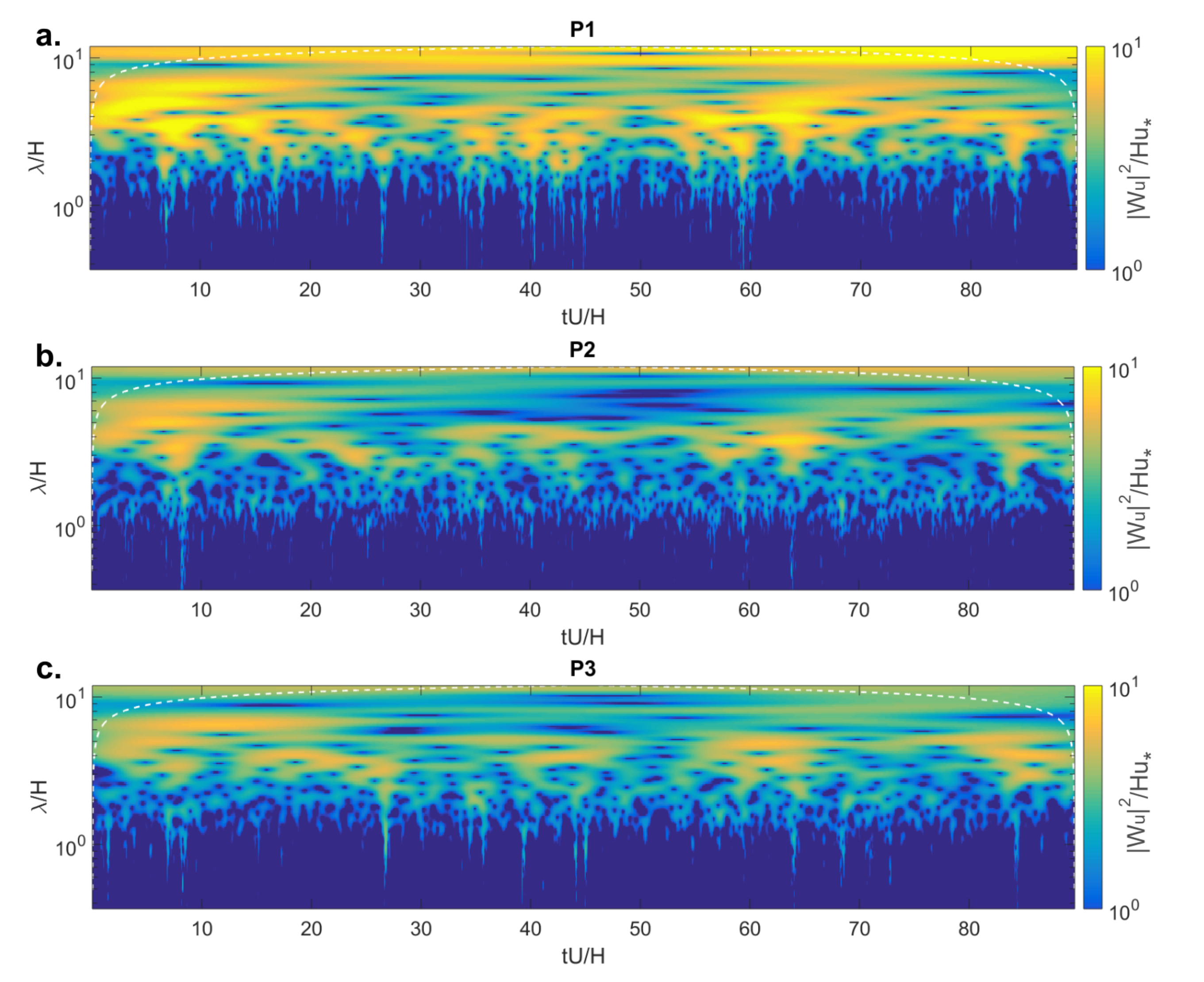
Since the sediment ejection is a quasi-steady flow, then the local wavelet spectrum in the experiment E1, after the spill of fine sediment mixture, was implemented to analyze the $u^{\prime }$ and $w^{\prime }$ velocity components in the three points of the sediment ejection, P1, P2 and P3 (Figure 12 and Figure 13). The wavelet spectra ${\left|Wu\right|}^2$ and ${\left|Ww\right|}^2$, corresponding to the wavelet spectra for $u^{\prime }$ and $w^{\prime }$ velocity fluctuations, respectively, were made dimensionless with dimensionless with $H{u}_{*}$, as shown in Figure 12 and Figure 13. The spectra have $\lambda /H$ in vertical axes and $tU/H$ in horizontal axes, where $\lambda$ is the wavelength calculated as $\lambda =U/f$, f is frequency and $tU/H$ is the dimensionless time. Wavelet analysis allows for seeing the variations of the power spectrum over time, i.e., with this analysis, a turbulent structure is determined and the time the structure is present in the measurement time. In the streamwise direction, upstream of sediment ejection, P1, the energy is concentrated for $\lambda =10H$, for a long period of time, $10<tU/H<82$ (Figure 12). This wavelength is associated with a frequency of 0.06 Hz. According to the power spectrum shown in Figure 11e, it is a structure corresponding to a large-scale motion, i.e., this large-scale is present in almost all the time of the measurement time. In points P2 and P3, there is concentration of energy at this wavelength (frequency), but it is less intense than at P1, whereas, for $\lambda =5H$ and $\lambda =4H$, there is a concentration of energy at all the measurement points, P1 to P3. This wavelength is associated with frequencies of 0.13 Hz and 0.16 Hz, corresponding to large-scale motions (Figure 11d–f). However, this structure is present only at certain points in time; the period most frequent is $tU/H\sim 50$ (Figure 12a–c).

The wavelet spectrum for vertical fluctuation shows energy concentrations in P2 and P3 higher than those of P1; the highest concentration of energy is that of P2. This wavelet spectrum shows that, at point P2, during the entire measurement time, the vertical component of sediment ejection dominates, as shown in the spectrum of Figure 9b. According to the wavelet spectrum, Figure 13b, $\lambda =10H$ has a high energy concentration for $10<tU/H<82$. That wavelength corresponds to the frequency 0.06 Hz and is associated with a large scale of motion for P2 and P3 (Figure 11b,c). In addition, for $\lambda =5H$, $4H$, and $3H$, there is a concentration of energy at points P2 and P3. This wavelength is associated with frequencies of 0.13 Hz, 0.16 Hz, and 0.21 Hz, respectively, corresponding to large-scale motions (Figure 11d–f). However, these structures are present only at certain points in time, the period most frequent is $tU/H\sim 40$ (Figure 12a–c).

4. Discussion

The coherent structure in turbulence flows have been researched by [16,18,19,36,39] in open channels with permeable and impermeable beds, considering a steady flow. One methodology has been to analyze the Reynolds shear stress in quadrants of the Cartesian plane, with $u^{\prime }$ and $w^{\prime }$ and their distribution is described as an ellipse of negative slope and a turbulent event has a high probability to be in the quadrant $Q2$ and $Q4$, while $Q1$ and $Q3$ have a low probability of occurrence. In this study, we can see the same distribution of Reynolds shear stress in the case of open channel without fine sediment deposited into the bed (E0). However, the interaction between surface and subsurface flow in E1, after the spill of pumicite mixture, causes the analysis to change. The sediment ejection generates a quasi-steady flow from the bed toward the water column, where the vertical velocity component is higher than the streamwise velocity component, i.e., the turbulent interactions in $Q1$ and $Q3$ for that structure has a higher probability than in other research.

Furthermore, for isotropic turbulence in smooth open channel flow, Taylor’s frozen turbulence hypothesis has been validated by [13,20,40] and others. Taylor’s frozen turbulence hypothesis is also validated in experiment, E0, for $z/H>0.1$. However, Ref. [41] recognizes the limitations of applying the Taylor’s hypothesis. They considered an uncertainty for $z/H<0.1$ because, in this region, the mean velocity and local velocity can diverge. Then, in experiment E0, the velocity difference between P1 and P2 for $z/H<0.1$ is associated with a divergence of gravel pore velocities, so that, near the permeable bed, the Taylor’s frozen turbulence hypothesis is invalidated, and these results are according to [41].

In experiment E1, fine sediment ejections are quasi-steady flows from the bed. Turbulence patterns change and turbulence becomes anisotropic because sediment ejection has a dominant vertical velocity. In this case, Taylor’s frozen turbulence hypothesis is also invalidated.

The power spectrum density in open channels has been reported by [42,43,44]. They have validated the $-5/3$ slope in the measured spectra and show a greater spectral density of the streamwise component than the spanwise and vertical components. However, in this study, for the experiment E0, in the production zone, there is a greater spectral density of the streamwise component than the vertical component, but in the inertial subrange both components have a spectral density of similar magnitude. Conversely, in experiment E1, since the sediment ejection has a dominant upward movement, the spectral density changes. Upstream of the sediment ejection, at P1, in the production zone, the spectral density for streamwise component is greater than the vertical fluctuation component and the spectrum densities in both components are greater than the spectral density in experiment E0, whereas, in the center of the ejection, at P2, in the production zone and in the inertial subrange, the spectral density for vertical fluctuation component is greater than the spectral density for streamwise components. Downstream of the ejection in experiment E1, P3 can be considered as a downwelling point. It is important to note that sediment ejection increases the spectral energy, both in the production zone and in the inertial subrange.

Coherent structures of turbulence in open channels have been characterized by their sizes, such as small-scale motion, large-scale motion, and very-large scale motion by [13,20]. Streamwise scales of $3H$ and $10H$ allow coherent structures in these experiments to be classified as large-scale, i.e., hairpin vortex, and very large-scale motion, i.e., super streamwise vortex. Ref. [20] implemented the wavelet analysis to detect high concentrations of energy over time and their scale of motion, finding high concentrations of energy in $\lambda =3H$ and $\lambda =10H$, i.e., they reported hairpin vortices and super stream vortices; however, they did not show the influence cone, so the presence of the super stream vortices is not clear. The large-scale motion and the very large-scale motions find in this research are not the same coherent structures reported by [13,20] because the pattern of the sediment ejection has a dominant vertical component. In addition, the energy concentration changes with the measurement position inside the sediment ejection.

The interaction between ejections, sweeps, outward, and inward interactions generates turbulent structures such as horseshoe vortices, hairpin vortices, shedding vortices, etc. Those turbulent structures can move sediment away from where they occurred, i.e., they can generate erosion or scour [45]. Interactions such as ejections and sweeps are more common in open channels; however, in the experiments presented in this article, this is not entirely true. Outward and inward interactions are more frequent than in open channels. Furthermore, pumicite is a fine cohesive material, so mechanisms such as particle rolling, sliding, and saltation were not observed in the present experiments. Therefore, no erosion or scour was observed due to the sediment expulsion. However, there is a constant interaction between the surface and subsurface flow. This dynamic is relevant considering that the fine material can be, for example, mining materials and, therefore, a constant exchange of toxic material can be generated from the hyporheic zone to the surface flow.

The experimental scale is small compared with natural environments, but the dimensionless parameters in the experiments presented in this article on the basis of the flow and sediment transport phenomena in mountain streams are believed to be correct. The dimensionless parameter $H/D_g=$ 6.7 of the experiments is representative of macroroughness flow and there is no bedload transport, that is, ${\tau }_{*}=0.00006<{\tau }_{*c}=0.035$, where ${\tau }_{*}$ is the dimensionless shear stress, ${\tau }_{*}=u_{*}^2/\left(gR{D}_g\right)$, and ${\tau }_{*c}$ is the critical shear stress for the incipient motion of the sediment, with $R=({\rho }_s-\rho )/\rho$, ${\rho }_s$ and $\rho$ are the sediment and water density, respectively [38]. However, the dimensionless parameter that is essential for this article is $u_e/w_s$, where $u_e$ is the entrainment velocity and $w_s$ is the fall velocity of the fine sediment [10]. The dimensionless parameter $u_e/w_s>1$ would make entrainment possible. The flow average vertical velocity $<w>$ in P2 is 0.007 m/s (Figure 9) and $w_s$ of the pumicite is 0.005 m/s, so, if $u_e$ is equal to $<w>$, $<w>/w_s>1$ and there is entrainment of the pumicite to the surface flow. The value of $w/U$ in P2 observed in Figure 9 is in the order of 0.15, which shows that a significant part of the subsurface flow appears in the surface flow.

5. Conclusions

Fine sediment, such as pumicite, between the pores of a gravel river bed, can reduce the permeability and the initial porosity of the bed, modifying the roughness and hydraulic parameters of the subsurface flow. Pumicite has a low density, generating changes in the interaction between the subsurface and surface flow. These interactions are mass, momentum, and energy exchange, so the decrease of permeability of the gravel layer can generate an increase of vertical velocity and the turbulence intensities in the surface layer. Additionally, low velocities in the streamwise direction and high vertical velocities can break the streamwise structures associated with secondary currents near the bed and sediment ejections can be seen.

The sediment ejections change the patterns of turbulent structures and the distribution of the turbulence interactions, which means that the flow does not have a typical rough wall open channel flow turbulence. Additionally, the sediment ejections increase the energy both in the production zone and inertial subrange. Within the ejection, the vertical velocity component has the highest increase of energy in the center of the ejection. The sediment ejections could vary with the granular size of the subsurface layer and the density of the fine material, i.e., the low-density fine material in the subsurface layer encourages the presence of sediment ejections from the bed.

As future work, we will continue to evaluate the turbulent structures associated with sediment ejections in the presence of surface and subsurface flows. Fine sediments, with higher densities will be considered, for example, mining materials, such as tailings or metal concentrates, to evaluate the effect of particle density on the dynamics of the ejection. To characterize both spanwise and the sediment ejection in 3D, we will implement the technique Stereo PIV.