Article

Modeling Soil Nitrate Accumulation and Leaching in Conventional and Conservation Agriculture Cropping Systems

by
Nicolò Colombani
1,
Micòl Mastrocicco
2,*,
Fabio Vincenzi
3 and
Giuseppe Castaldelli
3
1
SIMAU-Department of Materials, Environmental Sciences and Urban Planning, Polytechnic University of Marche, Via Brecce Bianche 12, 60131 Ancona, Italy
2
DiSTABiF-Department of Environmental, Biological and Pharmaceutical Sciences and Technologies, Campania University “Luigi Vanvitelli”, Via Vivaldi 43, 81100 Caserta, Italy
3
SVeB-Department of Life Sciences and Biotechnology, University of Ferrara, Via L. Borsari 46, 44121 Ferrara, Italy
*
Author to whom correspondence should be addressed.
Water 2020, 12(6), 1571; https://doi.org/10.3390/w12061571
Submission received: 25 January 2020 / Revised: 13 May 2020 / Accepted: 29 May 2020 / Published: 31 May 2020

Abstract

:
Nitrate is a major groundwater inorganic contaminant that is mainly due to fertilizer leaching. Compost amendment can increase soils’ organic substances and thus promote denitrification in intensively cultivated soils. In this study, two agricultural plots located in the Padana plain (Ferrara, Italy) were monitored and modeled for a period of 2.7 years. One plot was initially amended with 30 t/ha of compost, not tilled, and amended with standard fertilization practices, while the other one was run with standard fertilization and tillage practices. Monitoring was performed continuously via soil water probes (matric potential) and discontinuously via auger core profiles (major nitrogen species) before and after each cropping season. A HYDRUS-1D numerical model was calibrated and validated versus observed matric potential and nitrate, ammonium, and bromide (used as tracers). Model performance was judged satisfactory and the results provided insights on water and nitrogen balances for the two different agricultural practices tested here. While water balance and retention time in the vadose zone were similar in the two plots, nitrate leaching was less pronounced in the plot amended with compost due to a higher denitrification rate. This study provides clear evidence that compost addition and no-tillage (conservation agriculture) can diminish nitrate leaching to groundwater, with respect to standard agricultural practices.

1. Introduction

Groundwater nitrate (NO3) pollution below croplands is a long-term legacy [1,2,3], and not surprisingly, NO3 is considered the most widespread inorganic pollutant around the world [4,5]. Moreover, Ascott et al. [6] have recently pointed out that the vadose zone is an important stock of NO3 and this transient stock should be accounted for in N budgets for more robust policymaking. In fact, long residence times in the vadose zone may delay the impact of changes in agricultural practices on groundwater quality even in lowland catchments [7,8].
The mathematical formulation and the solutions of transient transport and transformation from urea hydrolysis, ammonification, nitrification, and denitrification have been used for decades in soil hydrology [9,10,11,12]. The numerous reactions involved in the N cycle in soils are substantially driven by different microbial consortia that are usually modeled via first-order reaction kinetics, like in the HYDRUS-1D model [13]. Although, there are many other numerical models that have been specifically developed for N species transformation and transport in variably saturated media, such as DAISY [14] or COUP [15], the model choice is often driven by the aims of the research. In fact, agronomic empirical models are usually devoted to quantifying crop yield fertilizer plant-uptake and C and N soil turnover, like the EPIC model [16], while physically based models like HYDRUS-1D are better suited for porewater fluxes, nitrogen balance and leaching calculations (nitrification, denitrification, volatilization, mineralization). In this case, the aim of the research is to quantify the driving mechanisms of nitrate leaching; thus, the physically-based model HYDRUS-1D was selected. However, despite the large capabilities reached by physically-based models, N transformation processes are intrinsically complex and difficult to quantify in field conditions since they are driven by site-specific parameters such as soil water content, temperature, root presence, and redox conditions [17]. For the above-mentioned reasons, physically-based models need to be calibrated and validated against a large amount of field data to be considered robust and to effectively reproduce the ongoing site-specific N transformation processes [18,19,20]. Thus, the last challenge is to use these well-established numerical models at well-equipped field sites and over long-term periods, e.g., different hydrological years and different crop growing seasons, to quantify the effects induced by different agricultural practices on both soil hydrology and N transformations. Otherwise, without the quantification capacity for a field-validated numerical model, it would be very challenging to infer how much soil N leaching is affected by agricultural practice changes.
In this study, two experimental plots located in the lower end of the Po river plain (Italy), were monitored and modeled for a period of 974 days (3 cropping seasons). One plot was amended at the beginning of the study with 30 t/ha of compost, amended with synthetic fertilizers and cultivated using no-tillage practices, following the conservation agriculture indications [21,22], while the other one was run with a standard approach, namely, using synthetic fertilizers and deep tillage practices. Here, the numerical model HYDRUS-1D was calibrated and validated versus field-observed data to infer if soil hydrology and N transformations were substantially changed by the introduction of conservation agriculture practices. As far as the authors are aware, this is the first study that uses a combination of continuous soil moisture sensors, high-resolution tracer profiles, and soil NO3 content to calibrate and validate a numerical model in a compost/no-tillage field experiment. In fact, other similar studies were only calibrated and validated versus observed soil NO3 content [23,24] or discontinuous soil moisture content and soil N content [25].

2. Materials and Methods

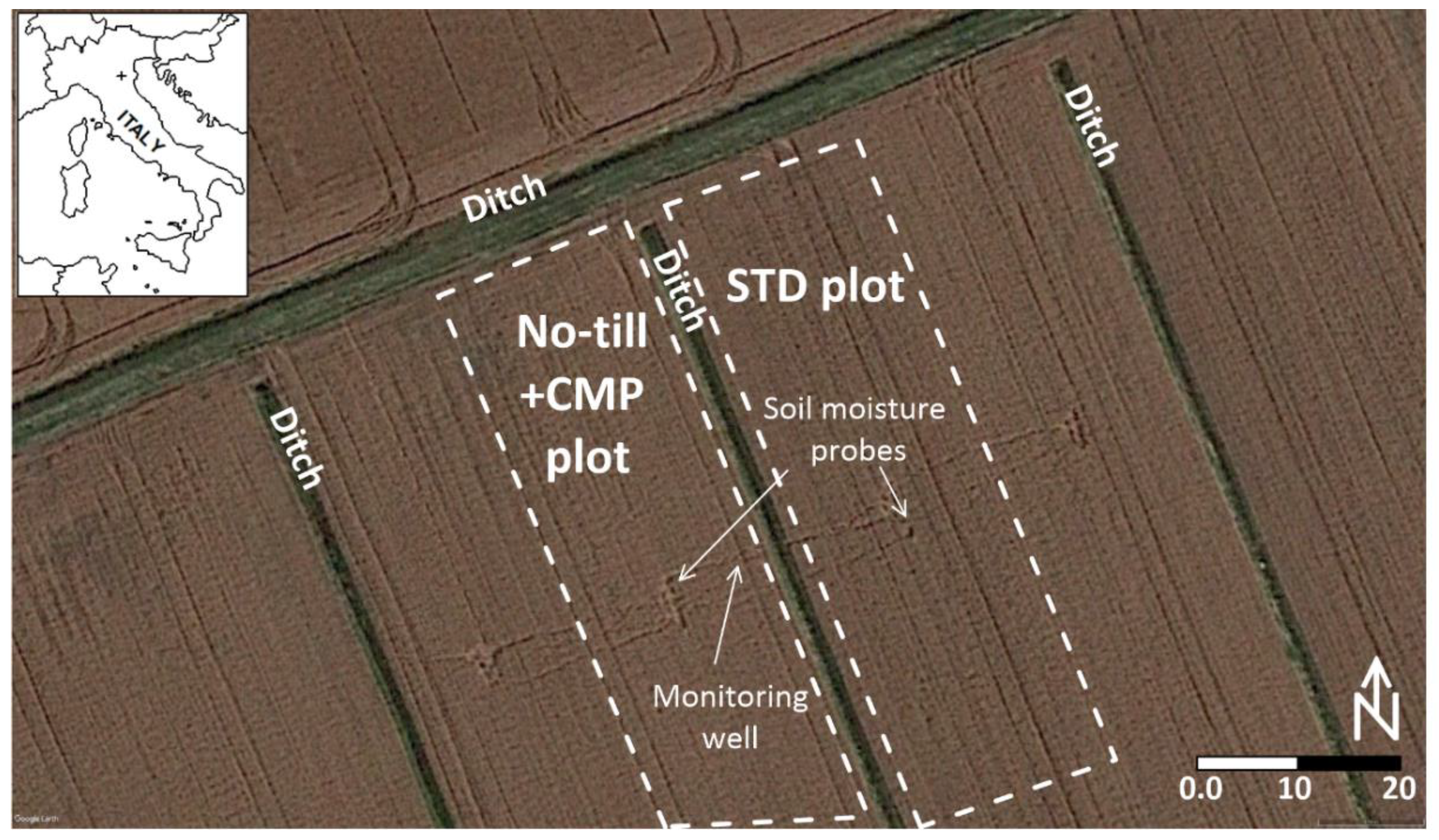
2.1. Site Location and Characterization

The agricultural test site is located in the Po River plain near the city of Ferrara (Northern Italy) at the following coordinates: 44°47′41″ N and 11°42′20″ E (Figure 1). The soil is classified as hypocalcic haplic calcisol. The site has been cultivated with a rotation of cereals (maize and winter wheat) and a precession of beetroot. It is representative of large portions of the lower Po river valley.
The site was investigated as part of a research project supported by the Rural Development Programme of the Emilia-Romagna Region (PSR 2014–2020), which aims to reduce the environmental impact of agricultural practices by comparing the use of compost and no-tillage techniques versus the classic fertilization and tillage techniques. A plot of 2500 m2 was amended with 30 t/ha of compost incorporated in the soil with a minimum-tillage technique (15 cm). After that, the plot underwent a no-tillage practice (No-till+CMP plot) for the whole duration of the experiment, while another plot was cultivated with classic fertilization and tillage practices (STD plot). The field was cultivated with (i) winter wheat, seeded on 30 October 2016 and harvested on 26 June 2017; (ii) maize, seeded 7 April 2018 and harvested on 24 August 2018; (iii) winter wheat, seeded on 20 October 2018 and harvested on 28 June 2019. N fertilization was done via different fertilizers, as shown in Table 1, while compost was incorporated in the No-till+CMP plot at the beginning of the experiment via minimum tillage moldboard (10–15 cm deep).
A series of 5 soil samples (1 cm diameter and 20 cm long-cores) were collected using an Eijkelkamp Soil & Water M04 model hand-driven gouge auger corer (Giesbeek, The Netherlands) with a diameter of 30 mm. As it causes minimal disturbance of the sample, the gouge auger is frequently applied in profile research. Core samples were taken randomly in the field 10 m from each other at a depth of 0–20, 50–70 and 90–110 cm below ground level (b.g.l.) to assess the horizontal and vertical variability of the soil’s physical properties, NO3, and NH4+ concentrations in both experimental plots. The collected soil samples were stored in polyethylene (PE) bottles and immediately frozen at −18 °C until analyzed. NO3 was analyzed with a Technicon Autoanalyser II, while NH4+ was analyzed using a double beam Jasco V-550 UV–vis spectrophotometer.
Figure 2 depicts the meteorological conditions recorded during the study period, using data from a meteorological station located near the field site. Two irrigation events of 50 mm/day, performed during maize flowering with sprinklers (28 June and 13 July 2018), were also included. The reference potential evapotranspiration rate (Et0) was calculated using the Penman–Monteith equation [26]. The groundwater heads were monitored every 30 minutes and then averaged on a daily basis using a Soil & Water Diver Micro® water level data-logger (Eijkelkamp, Giesbeek, The Netherlands), corrected for atmospheric pressure changes and placed in a 4.0-m deep piezometer situated between the two plots.
An array of Watermark® soil moisture sensors (Irrormeter Company, Riverside, CA, USA) was vertically inserted at 30, 60, and 90 cm b.g.l. into augered holes in each experimental plot. The soil moisture sensors were used to monitor the matric potential (measurement range 0–25 m of water). A copper-constantan thermocouple was inserted adjacent to each soil moisture probe to compensate for the raw measurements of soil temperature since the probes are sensitive to temperature changes. Moreover, to better observe the matric potential variation induced by the plants’ roots transpiration, a TEROS 21® soil water potential sensor (Meter Environment, Pullman, WA, USA) was placed at 30 cm b.g.l. in both experimental plots (measurement range 0.9–100 m of water). The principal soil parameters (Table 2) were sourced from a previous study [27], while the mineralogical composition of these soils is quartz, K-feldspar, plagioclase, and calcite, associated with small amounts of dolomite; the clay minerals are mainly smectite, chlorite, serpentine, and mixed layers [28]. Bromide (Br) was applied at the beginning of the project (30 October 2016) at a concentration of 1000 mg/l. More details can be found in Colombani et al. [8].

2.2. Flow and Transport Modelling Approach

The finite element model HYDRUS-1D [13] was selected for simulating the one-dimensional movement of water in variably saturated media. The code solves Richards’ equation for saturated–unsaturated water flow via a numerical algorithm under the assumption that the air phase is negligible and thermal gradients can be ignored in the water flow process. Since an undisturbed soil column collected at this field site [27] was already successfully simulated using the dual-porosity approach proposed by Durner [29], the same approach was used to simulate this field experiment. This method splits the porous medium into two overlapping regions, and for each of these regions, a van Genuchten–Mualem type function [30] of the soil hydraulic properties is used.
The standard advection–dispersion equation (ADE) for dissolved species transport with linear sorption was selected to simulate the fate and transport of N species in the vadose zone. The actual root water uptake was simulated using the Feddes water stress response function [13]. Variable crop heights depending on the phenological state and maximum rooting depths, defined by visual inspection during core sampling, were used as input values. Passive nutrient uptake was simulated by multiplying root water uptake with the dissolved nutrient concentration for soil solution concentration values below a threshold concentration (Crmax). Passive nutrient uptake is thus zero when Crmax equals to zero, while when the concentration is lower than Crmax, the solute is removed from the model, or when the concentration is higher than Crmax, the solute is left in the soil. The Crmax was set very high for nutrients (1000 mg-N/dm3) and lower for Br (100 mg/dm3).

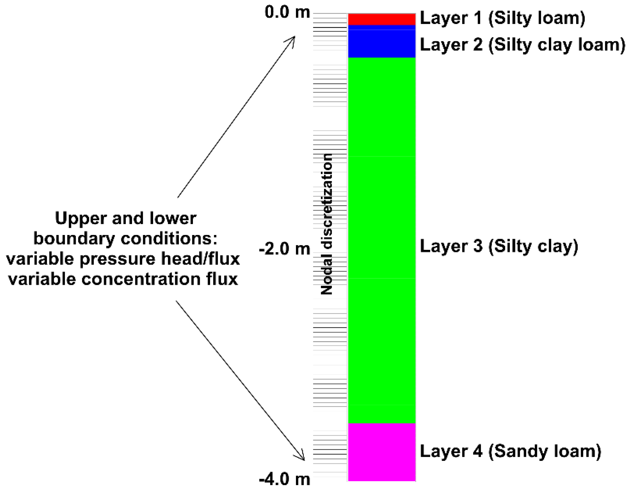
2.3. Flow and Transport Boundary Conditions

The numerical grid was discretized in 101 nodes of 40 mm each to form a regular grid 4.0 m deep (Figure 3). At the soil surface, a variable pressure head/flux boundary condition was selected to replicate variations in the infiltration rate due to different rainfall intensities. As a bottom boundary condition, a variable pressure head/flux boundary also was specified.
In the transport model, a third-type (Cauchy) concentration flux boundary condition, with user-specified liquid phase concentration of the infiltrating water, was selected as upper and lower boundaries.
The reactive network used to simulate the sequential transformations of the N species (from urea to NH4+, NO2, and NO3) was the one initially proposed by van Genuchten [31], coupled with linear sorption for NH4+ and NH3 volatilization via a first-order reaction [13]. The organic N mineralization rate of both compost and soil organic matter was accounted for using a zero-order production rate for urea, here assumed as a generalized organic N source. NH4+ and NO3 deposition from precipitations was included to account for a rate of 25 kg-N/ha/year [32], which is an intermediate value between the lower 13 kg-N/ha/year [33] and upper 34 kg-N/ha/year [34] estimates for northern Italy. The nutrient sources and amount were specified following the data shown in Table 1. Tillage operations can alter the Ks of the topsoil immediately after, but there was not enough data on Ks variations to include such complexity; thus, Ks was treated as constant throughout the project. The initial species concentrations were linearly interpolated throughout the model profile using the observed concentrations collected every 50 cm. The linear sorption coefficient for NH4+ (2.14 × 10⁻⁵ dm3/mg-N), ammonification rate (0.28 1/day), nitritation rate (0.12 1/day) and nitratation rate (5.9 1/day) were sourced from Mastrocicco et al. [27], while the first-order volatilization rate (0.66 1/day) was sourced from laboratory experiments on NH3 volatilization conducted in nearby fields [12]. Diffusion values such as molecular diffusion in water (1.0e−5 m2/day) and in air (1.52 m2/day) and the Henry equilibrium distribution constant between liquid and gaseous phases for NH3 (0.01) were kept constant in all horizons.

2.4. Model Calibration and Validation Procedure

The model calibration target was to minimize the differences between the observed and calculated values for matric potential and Br, NO3, and NH4+ concentrations from the plots in the first two cropping years (from October 2016 to September 2018). The model was then validated using the observations of the last cropping season (from September 2018 to June 2019). The flow and transport parameters were assumed to be homogeneous throughout the soil column; thus, they were kept constant within each model, except for vertical dispersivity (λv). The flow and transport model parameters were automatically adjusted via an inverse modeling procedure present in HYDRUS-1D. The latter uses a Marquardt–Levenberg type algorithm to optimize each parameter versus an objective function made by all the available observations and their respective weights [13]. The optimized flow parameters were residual soil water content (Qr) and the saturated soil water content (Qs) of the van Genuchten [30] parametric functions in the 4 layers constituting the model domain, for a total of 8 parameters. The optimized transport parameters were λv (m) and denitrification rate (1/day). Other reaction parameters listed in Table 3 were sourced by a similar model previously developed for this soil [27].
The degree of model calibration was assessed by calculating and comparing the determination coefficient (R2) and modeling efficiency (EF) calculated according to Nash and Sutcliffe [35]:
E F = 1 j = 1 n ( O j P j ) 2 j = 1 n ( O j O ) 2 ,
where Pj is the calculated value corresponding to the observed Oj, and O is the mean value of the observed data.

3. Results and Discussion

3.1. Flow Model Results

The flow model was calibrated versus the continuous monitoring of in situ matric potential (Figure 4). Given that the observed values in the two different experimental plots were not dissimilar, it was decided to average the daily values at the same depth to calibrate a single flow model capable of reproducing the soil water fluxes in both plots. The dual-domain approach employed here was indispensable to avoid water ponding and runoff, which was not observed after extreme rainfall events, like the one recorded in September 2017 (see Figure 2).
The latter caused a sudden decrease of matric potential at all monitored depths (Figure 4) that would not have been as well-represented by single porosity, which cannot allow rapid infiltration in low hydraulic conductivity (Ks) soil despite the elevated precipitation rates [36]. The soil retention curve parameters (Table 3) are essentially the ones retrieved from a previous intact soil column experiment performed in the same field site [27], and the good model performance (R2 = 0.90 and EF = 0.85) proves that undisturbed soil column experiments can be used to provide reliable estimates of soil retention parameters provided the size of the column is large enough to account for macroporosity at the plot scale [37]. From Figure 4, it is also evident that the matric potential was influenced not only by the roots’ water uptake but also by meteorological conditions that indeed contributed to decreasing matric potential during summer 2017 and spring 2018 via frequent rainfall events.

3.2. Nonreactive Transport Model Results

Figure 5 shows the results of the natural gradient tracer test started at the beginning of the project and the Br concentrations simulated by the nonreactive transport model. The model was fitted versus the observed Br concentrations sourced from a previous study on environmental tracers [8]. The center mass was recovered at approximately −0.4 m b.g.l. in both experimental plots, near the maximum plowing depth. Thus, it was decided to calibrate a single nonreactive transport model capable of reproducing the solute advection and dispersion in both plots. It should be noticed that the water table was always lower than −0.8 m b.g.l. and vertical solute transport in the vadose zone was much slower than in saturated conditions. Moreover, the data and their modeling allow us to infer that the conservation agriculture practices did not significantly alter the solute transport in the vadose zone with respect to standard practices, at least according to the available data. A change in physical parameters influencing solute transport, e.g., Ks, should be expected only after different years from the introduction of the conservation agriculture practices [38,39].
The vertical distribution of Br concentration was well fitted using the standard ADE equation (Figure 5), with a calculated R2 of 0.88 and an EF of 0.81. Thus, for the principle of parsimony in numerical models [40], there was no need to use more complex approaches like the mobile−immobile physical nonequilibrium approach [41]. The obtained λv values are relatively large in the upper soil layers (Table 4), indicating a greater soil heterogeneity in the plowed horizon; these values are in line with the value of 20.3 mm previously obtained for the column experiment [27]. In addition, the obtained values are also within the range of the observed λv values for tilled agricultural soils [39]. Finally, it should be mentioned that Crmax for Br largely influences the simulation results, so after a trial and error calibration (since Crmax cannot be automatically calibrated), a best-fit value of 103 mg/dm3 was obtained. The cumulative mass taken up by roots was 22.1% of the Br mass, a value generally consistent with the literature data of 8.1% [41], 10.0% [42], or even higher (from 11% to 38%) [43,44]. Nevertheless, this parameter should be better characterized in future tracer studies and included in inverse modeling procedures, given that a simple sensitivity analysis variating the calibrated Crmax value of ± 15% shows very different calculated Br concentration profiles (Figure 5).

3.3. Reactive Transport Model Results

From Figure 6, the vertical profiles of NO3 in the STD experimental plot were reproduced with sufficient quality by the numerical model, with a calculated R2 of 0.68 and an EF of 0.59, although the model failed to accurately simulate NO3 concentrations between 0.5 and 0.7 m b.g.l., which is below the interface between the tilled and untilled soil horizons.
In addition, the No-till+CMP model suffered from poor model performance (Figure 6), with a calculated R2 of 0.69 and an EF of 0.58. This could be due to a number of reasons, such as root distribution heterogeneities in both space and time, seasonal variation of organic N mineralization rate that was taken as constant here, complex behavior of the uptake rate by plants’ roots modeled here as passive root water uptake, variations of soil denitrification determined by seasonal variation of substrates’ availability, and soil moisture and saturation. Nevertheless, both simulations were capable of capturing the overall NO3 and NH4+ fate in the subsurface, and in particular, the NO3 concentrations were always lower in the No-till+CMP respect to the STD experimental plot, except for the initial season when the compost was incorporated into the topsoil (Figure 7). This is a clear indication that the conservation agriculture practices have less impact on the environment than the standard ones, in agreement with previous studies [24,25]. In fact, NO3 concentrations below the maximum rooting zone (0.9 m b.g.l.) were always lower in the No-till+CMP experimental plot.
Moreover, the organic N mineralization rates (Table 5) were capable of producing ≈45 Kg-N/ha/year for the No-till+CMP plot and ≈5 Kg-N/ha/year for the STD plot. The large difference between the two N mineralization rates is due to the low reactivity of soil organic matter in intensively cultivated fields [45]. In the No-till+CMP, despite the higher organic N mineralization rate induced by the compost addition, the large pool of available organic carbon also triggered denitrification. In fact, the calibrated values for the No-till+CMP plot are nearly two times higher than the denitrification rate used for the STD plot. Besides, to achieve a good calibration, denitrification was also activated in Layer 3 of the No-till+CMP model (Table 6).
These values are in agreement with previous experiments that have reported limited denitrification for STD soil [27] and enhanced denitrification rates when the same soil is amended with labile organic substrates, such as acetate [45] produced by roots exudates, mineralization of crop residues, or organic soil improvers such as compost. Finally, Figure 8 shows the cumulative N mineralization and denitrification rates calculated for both experimental plots. Here, it is evident that denitrification was able to remove up to 180 kg-N/ha during the 3 cropping seasons in the No-till+CMP plot, while only 120 kg-N/ha was produced by N mineralization processes. In the STD plot, denitrification was able to remove only 53 kg-N/ha, while less than 13 kg-N/ha was produced by N mineralization processes.
An elevated denitrification rate in organic-matter-amended soils is seen as a positive mechanism for the protection of surface and ground waters from diffused NO3 pollution. However, from an agronomical perspective, it is evidently a negative feature, as this also means a net loss of N fertilizer from the field. Therefore, with the aim of developing management strategies for both environmental and economic sustainability, the model results shown in Figure 8 have to be considered by taking into account both perspectives. To do so, it must be considered that denitrification is not an independent process, but is fully integrated into the N cycle in agricultural soils. In fact, in soil, when water saturation leads to O2 scarcity, anaerobic processes are favored and denitrification becomes important [45]. The heterotrophic denitrification rate is then constrained by the availability of both organic substrates and NO3. Thus, in the presence of great availability of labile organic substrates, such as in the No-till+CMP plot, the mean yearly denitrification rate is higher than for standard agricultural practices (Table 6). However, from a long-term perspective, the adoption of agriculturally conservative practices, aimed at increasing and maintaining soil organic matter, would lead to a slow but continuous release of mineral N (Table 6). This would allow the reduction of the intensity of synthetic fertilizer applications, leading to basal N concentrations much lower than the peak values that usually are recorded below agricultural lands fertilized with synthetic urea, as done in conventional agriculture. A situation of this type, characterized by low basal NO3 concentrations, would correspond to a limitation of electron acceptors for denitrification and, therefore, to a reduction of N losses from the field. Therefore, the increase of soil organic matter has a dual positive role: in the short term, to enhance denitrification as a buffer to prevent losses of NO3 to surface and ground waters, and in the long term, to increase the efficiency of N fertilization in agriculture by increasing the basal N supply, a feature that allows the reduction of the intensity of synthetic fertilizers distribution. This could avoid the formation of NO3 excess in topsoil, preventing denitrification and N losses to the atmosphere in the form of both N2 gas and hazardous N protoxide. Finally, it must be mentioned that the main limitation of the proposed approach, and in general of the physically-based models, is that the large amount of data necessary to calibrate and validate these models are extremely expensive and time-consuming, although, without such models, the quantification of mutual biogeochemical processes is extremely challenging. Future studies should focus on increasing the vertical resolution of samples to better capture the sharp concentration gradient fronts that can develop in these soils.

4. Conclusions

In this study, a HYDRUS-1D simulation of soil NO3 accumulation and leaching in conventional and conservation agriculture cropping systems was successfully calibrated and validated against continuously observed matric potentials, and against Br, NO3, and NH4+ soil profiles. The model provided insights on the water and nitrogen balance in the two monitored cropping systems, especially quantifying the long residence times in the vadose zone. This approach could be applied in many other lowland agricultural environments with similar soil and climate characteristics. One of the main outcomes is that the water balance and retention time in the vadose zone were similar in the two agricultural plots. However, to better identify advective and dispersive mechanisms, future studies should pay more attention to Br uptake rates by roots since this parameter largely controls Br soil concentrations. This study provides clear evidence that compost addition and no-tillage practices (conservation agriculture), but using the standard fertilization practices, can trigger the denitrification rate and thus diminish nitrate leaching into groundwater. Future studies should also focus on carbon cycling to add more information to the effective availability of electron donors for denitrification.

Author Contributions

Conceptualization, N.C. and M.M.; methodology, N.C. and M.M.; software, N.C.; validation, M.M.; formal analysis, F.V.; investigation, N.C. and F.V.; resources, G.C.; data curation, N.C. and M.M.; writing—original draft preparation, N.C.; writing—review and editing, M.M. and G.C.; visualization, N.C.; supervision, M.M. and G.C.; funding acquisition, G.C. All authors have read and agreed to the published version of the manuscript.

Funding

This work was financially supported by the Emilia-Romagna Region with the Project “Agronomic techniques for the prevention of nitrate pollution and the conservation of the organic matter” of the EIP-AGRI Operational Group “Nitrates Ferrara”, within the Rural Development Programme (PSR) 2014–2020.

Acknowledgments

The authors would like to thank Paolo Mantovi (CRPA) for providing the data on fertilizer type and quantity, and Marco Rivaroli and Luca Davì (Navarra Foundation for Agriculture) for sowing and harvest dates and tillage practices.

Conflicts of Interest

The authors declare no conflict of interest. The funders had no role in the design of the study; in the collection, analyses, or interpretation of data; in the writing of the manuscript, or in the decision to publish the results.

References

  1. Exner, M.E.; Hirsh, A.J.; Spalding, R.F. Nebraska’s groundwater legacy: Nitrate contamination beneath irrigated cropland. Water Resour. Res. 2014, 50, 4474–4489. [Google Scholar] [CrossRef] [PubMed] [Green Version]
  2. Tesoriero, A.J.; Duff, J.H.; Saad, D.A.; Spahr, N.E.; Wolock, D.M. Vulnerability of streams to legacy nitrate sources. Environ. Sci. Technol. 2013, 47, 3623–3629. [Google Scholar] [CrossRef]
  3. Jessen, S.; Postma, D.; Thorling, L.; Müller, S.; Leskelä, J.; Engesgaard, P. Decadal variations in groundwater quality: A legacy from nitrate leaching and denitrification by pyrite in a sandy aquifer. Water Resour. Res. 2017, 53, 184–198. [Google Scholar] [CrossRef]
  4. Fowler, D.; Coyle, M.; Skiba, U.; Sutton, M.A.; Cape, J.N.; Reis, S.; Sheppard, L.J.; Jenkins, A.; Grizzetti, B.; Galloway, J.N.; et al. The global nitrogen cycle in the twenty-first century. Philos. Trans. R. Soc. B 2013, 368, 20130164. [Google Scholar] [CrossRef] [PubMed]
  5. Gruber, N.; Galloway, J.N. An Earth-system perspective of the global nitrogen cycle. Nature 2008, 451, 293. [Google Scholar] [CrossRef]
  6. Ascott, M.J.; Gooddy, D.C.; Wang, L.; Stuart, M.E.; Lewis, M.A.; Ward, R.S.; Binley, A.M. Global patterns of nitrate storage in the vadose zone. Nat. Commun. 2017, 8, 1416. [Google Scholar] [CrossRef]
  7. Gerber, C.; Purtschert, R.; Hunkeler, D.; Hug, R.; Sültenfuss, J. Using environmental tracers to determine the relative importance of travel times in the unsaturated and saturated zones for the delay of nitrate reduction measures. J. Hydrol. 2018, 561, 250–266. [Google Scholar] [CrossRef]
  8. Colombani, N.; Mastrocicco, M.; Castaldelli, G.; Aravena, R. Contrasting biogeochemical processes revealed by stable isotopes of H2O, N, C and S in shallow aquifers underlying agricultural lowlands. Sci. Total Environ. 2019, 691, 1282–1296. [Google Scholar] [CrossRef]
  9. Rodríguez, S.B.; Alonso-Gaite, A.; Álvarez-Benedí, J. Characterization of nitrogen transformations, sorption and volatilization processes in urea fertilized soils. Vadose Zone J. 2005, 4, 329–336. [Google Scholar] [CrossRef]
  10. Hanson, B.R.; Šimůnek, J.; Hopmans, J.W. Evaluation of urea—Ammonium—Nitrate fertigation with drip irrigation using numerical modeling. Agric. Water Manag. 2006, 86, 102–113. [Google Scholar] [CrossRef]
  11. Li, Y.; Šimůnek, J.; Zhang, Z.; Jing, L.; Ni, L. Evaluation of nitrogen balance in a direct-seeded-rice field experiment using Hydrus-1D. Agric. Water Manag. 2015, 148, 213–222. [Google Scholar] [CrossRef] [Green Version]
  12. Castaldelli, G.; Colombani, N.; Tamburini, E.; Vincenzi, F.; Mastrocicco, M. Soil type and microclimatic conditions as drivers of urea transformation kinetics in maize plots. Catena 2018, 166, 200–208. [Google Scholar] [CrossRef]
  13. Šimunek, J.; Šejna, M.; Saito, H.; Sakai, M.; van Genuchten, M.T. The HYDRUS-1D software package for simulating the movement of water, heat, and multiple solutes in variably saturated media, Version 4.0. In HYDRUS Software Series 3; Department of Environmental Sciences, University of California Riverside: Riverside, CA, USA, 2008; Volume 3, p. 315. [Google Scholar]
  14. Hansen, S.; Abrahamsen, P.; Petersen, C.T.; Styczen, M. Daisy: Model use, calibration, and validation. Trans. ASABE 2012, 55, 1317–1333. [Google Scholar] [CrossRef]
  15. Jansson, P.-E.; Karlberg, L. Coupled Heat and Mass Transfer Model for Soil–Plant–Atmosphere Systems; Department of Civil and Environmental Engineering, Royal Institute of Technology: Stockholm, Sweden, 2001; p. 321. [Google Scholar]
  16. Izaurralde, R.C.; Williams, J.R.; McGill, W.B.; Rosenberg, N.J.; Jakas, M.Q. Simulating soil C dynamics with EPIC: Model description and testing against long-term data. Ecol. Model. 2006, 192, 362–384. [Google Scholar] [CrossRef]
  17. Zhu, Q.; Castellano, M.J.; Yang, G. Coupling soil water processes and nitrogen cycle across spatial scales: Potentials, bottlenecks and solutions. Earth-Sci. Rev. 2018, 187, 248–258. [Google Scholar] [CrossRef] [Green Version]
  18. Liang, H.; Qi, Z.; Hu, K.; Li, B.; Prasher, S.O. Modelling subsurface drainage and nitrogen losses from artificially drained cropland using coupled DRAINMOD and WHCNS models. Agric. Water Manag. 2018, 195, 201–210. [Google Scholar] [CrossRef]
  19. Banger, K.; Nafziger, E.D.; Wang, J.; Pittelkow, C.M. Modeling Inorganic Soil Nitrogen Status in Maize Agroecosystems. Soil Sci. Soc. Am. J. 2019, 83, 1564–1574. [Google Scholar] [CrossRef]
  20. Marjerison, R.D.; Melkonian, J.; Hutson, J.L.; van Es, H.M.; Sela, S.; Geohring, L.D.; Vetsch, J. Drainage and nitrate leaching from artificially drained maize fields simulated by the Precision Nitrogen Management model. J. Environ. Qual. 2016, 45, 2044–2052. [Google Scholar] [CrossRef] [Green Version]
  21. Knowler, D.; Bradshaw, B. Farmers’ adoption of conservation agriculture: A review and synthesis of recent research. Food Policy 2007, 32, 25–48. [Google Scholar] [CrossRef]
  22. Hobbs, P.R.; Sayre, K.; Gupta, R. The role of conservation agriculture in sustainable agriculture. Philos. Trans. R. Soc. B 2007, 363, 543–555. [Google Scholar] [CrossRef]
  23. Gerke, H.H.; Arning, M.; Stöppler-Zimmer, H. Modeling long-term compost application effects on nitrate leaching. Plant Soil 1999, 213, 75–92. [Google Scholar] [CrossRef]
  24. Iqbal, S.; Guber, A.K.; Khan, H.Z. Estimating nitrogen leaching losses after compost application in furrow irrigated soils of Pakistan using HYDRUS-2D software. Agric. Water Manag. 2016, 168, 85–95. [Google Scholar] [CrossRef]
  25. Asada, K.; Eguchi, S.; Tsunekawa, A.; Tsuji, M.; Itahashi, S.; Katou, H. Predicting nitrogen leaching with the modified LEACHM model: Validation in soils receiving long-term application of animal manure composts. Nutr. Cycl. Agroecosyst. 2015, 102, 209–225. [Google Scholar] [CrossRef]
  26. Allen, R.G.; Pereira, L.S.; Raes, D.; Smith, M. Crop Evapotranspiration. Guidelines for Computing Crop Water Requirements; FAO Irrigation and Drainage Paper 56; FAO: Rome, Italy, 1998; p. 15. [Google Scholar]
  27. Mastrocicco, M.; Colombani, N.; Soana, E.; Vincenzi, F.; Castaldelli, G. Intense rainfalls trigger nitrite leaching in agricultural soils depleted in organic matter. Sci. Total Environ. 2019, 665, 80–90. [Google Scholar] [CrossRef] [PubMed]
  28. Di Giuseppe, D.; Tessari, U.; Faccini, B.; Coltorti, M. The use of particle density in sedimentary provenance studies: The superficial sediment of Po Plain (Italy) case study. Geosci. J. 2014, 18, 449–458. [Google Scholar] [CrossRef]
  29. Durner, W. Hydraulic conductivity estimation for soils with heterogeneous pore structure. Water Resour. Res. 1994, 30, 211–223. [Google Scholar] [CrossRef]
  30. Van Genuchten, M.T. A closed-form equation for predicting the hydraulic conductivity of unsaturated soils. Soil Sci. Soc. Am. J. 1980, 44, 892–898. [Google Scholar] [CrossRef] [Green Version]
  31. Van Genuchten, M.T. Convective-dispersive transport of solutes involved in sequential first-order decay reactions. Comput. Geosci. 1985, 11, 129–147. [Google Scholar] [CrossRef]
  32. Rogora, M.; Arisci, S.; Marchetto, A. The role of nitrogen deposition in the recent nitrate decline in lakes and rivers in Northern Italy. Sci. Total Environ. 2012, 417, 214–223. [Google Scholar] [CrossRef]
  33. Castaldelli, G.; Soana, E.; Racchetti, E.; Pierobon, E.; Mastrocicco, M.; Tesini, E.; Fano, E.A.; Bartoli, M. Nitrogen budget in a lowland coastal area within the Po river basin (Northern Italy): Multiple evidences of equilibrium between sources and internal sinks. Environ. Manag. 2012, 52, 567–580. [Google Scholar] [CrossRef]
  34. Gumiero, B.; Candoni, F.; Boz, B.; Da Borso, F.; Colombani, N. Nitrogen Budget of Short Rotation Forests Amended with Digestate in Highly Permeable Soils. Appl. Sci. 2019, 9, 4326. [Google Scholar] [CrossRef] [Green Version]
  35. Nash, J.E.; Sutcliffe, J.V. River flow forecasting through conceptual models part I—A discussion of principles. J. Hydrol. 1970, 10, 282–290. [Google Scholar] [CrossRef]
  36. Nachabe, M.H. Estimating hydraulic conductivity for models of soils with macropores. J. Irrig. Drain. Eng. 1995, 121, 95–102. [Google Scholar] [CrossRef]
  37. Høgh Jensen, K.; Refsgaard, J.C. Spatial Variability of Physical Parameters and Processes in Two Field Soils Part II: Water Flow at Field Scale. Hydrol. Res. 1991, 22, 303–326. [Google Scholar] [CrossRef]
  38. Ismail, I.; Blevins, R.L.; Frye, W.W. Long-term no-tillage effects on soil properties and continuous corn yields. Soil Sci. Soc. Am. J. 1994, 58, 193–198. [Google Scholar] [CrossRef]
  39. Cade-Menun, B.J.; Bainard, L.D.; LaForge, K.; Schellenberg, M.; Houston, B.; Hamel, C. Long-term agricultural land use affects chemical and physical properties of soils from southwest Saskatchewan. Can. J. Soil Sci. 2017, 97, 650–666. [Google Scholar] [CrossRef]
  40. Hill, M.C. The practical use of simplicity in developing ground water models. Groundwater 2006, 44, 775–781. [Google Scholar] [CrossRef]
  41. Šimůnek, J.; Jarvis, N.J.; Van Genuchten, M.T.; Gärdenäs, A. Review and comparison of models for describing non-equilibrium and preferential flow and transport in the vadose zone. J. Hydrol. 2003, 272, 14–35. [Google Scholar] [CrossRef]
  42. Tilahun, K.; Botha, J.F.; Bennie, A.T.P. Bromide movement and uptake under bare and cropped soil conditions at Dire Dawa, Ethiopia. S. Afr. J. Plant Soil 2006, 23, 1–6. [Google Scholar] [CrossRef] [Green Version]
  43. Iragavarapu, T.K.; Posner, J.L.; Bubenzer, G.D. The effect of various crops on bromide leaching to shallow groundwater under natural rainfall conditions. J. Soil Water Conserv. 1998, 53, 146–151. [Google Scholar]
  44. Jemison, J.M., Jr.; Fox, R.H. Corn uptake of bromide under greenhouse and field conditions. Commun. Soil Sci. Plan. 1991, 22, 283–297. [Google Scholar] [CrossRef]
  45. Mastrocicco, M.; Colombani, N.; Castaldelli, G. Direct measurement of dissolved dinitrogen to refine reactive modelling of denitrification in agricultural soils. Sci. Total Environ. 2019, 647, 134–140. [Google Scholar] [CrossRef] [PubMed]
Figure 1. Satellite image sourced from Google Earth on 22 June 2017, with the location of STD (classic fertilization and tillage practices) and No-till+CMP (no-tillage practice) plots and of permanent instrumentation.
Water 12 01571 g001
Figure 2. Rainfall and irrigation events (blue line), groundwater head (red line), and reference evapotranspiration (black line) observed at the field site.
Water 12 01571 g002
Figure 3. Scheme of the numerical model setup used to simulate both the STD and No-till+CMP experimental plots.
Water 12 01571 g003
Figure 4. Comparison of the calculated (lines) and observed (open circles) pressure heads at different depths (cm b.g.l.). The −30 cm observation point belongs to Layer 2, while −60 cm and −90 cm observation points belong to Layer 3. Rainfall and irrigation events (blue line) are also plotted.
Water 12 01571 g004
Figure 5. Comparison of the calculated (black line) and observed (open circles) Br concentrations profiles collected on 27 March 2018 in both the experimental plots. Calculated Br concentrations using a Crmax of ±15% (dashed black lines) and minimum and maximum groundwater heads (dashed blue lines) are also plotted.
Water 12 01571 g005
Figure 6. Comparison of the calculated (lines) and observed (open symbols) NO3 and NH4+ concentrations profiles collected at selected dates in the STD experimental plot. Error bars represent the standard deviation over 5 replicates.
Water 12 01571 g006
Figure 7. Comparison of the calculated (lines) and observed (open symbols) NO3 and NH4+ concentrations profiles collected at selected dates in the No-till+CMP experimental plot. Error bars represent the standard deviation over 5 replicates.
Water 12 01571 g007
Figure 8. Comparison of the calculated cumulative N mineralization rate (upper panel) and denitrification rate (lower panel) for the No-till+CMP plot (black line) and for the STD plot (red line).
Water 12 01571 g008
Table 1. N fertilization events and rate in the STD and No-till+CMP experimental plots.
CropsDateFertilizerSTD Plot
(kg-N/ha)
No-till+CMP Plot
(kg-N/ha)
Winter wheat13 October 2016NH4NO34092 *
23 February 2017NH4NO38540
03 April 2017Urea4646
Maize29 March 2018(NH4)3PO43636
07 April 2018NH4H2PO433
30 April 2018Urea115115
11 May 2018Urea115115
Winter wheat10 October 2018(NH4)3PO43636
27 February 2019NH4NO35454
04 April 2019Urea6464
* considering the N use efficiency from compost equals to 40%.
Table 2. Sediment parameters and their standard deviation from quintuplicate samples. Data sourced from Mastrocicco et al. [27].
Parameter0–20 (cm b.g.l.)50–70 (cm b.g.l.)90–110 (cm b.g.l.)
Grain size (%)
Fine Sand (0.63–2 mm)10.1 ± 1.88.1 ± 0.89.0 ± 1.3
Silt (2–63 μm)55.8 ± 2.556.9 ± 3.547.5 ± 4.1
Clay (<2 μm)34.1 ± 3.035.0 ± 2.443.5 ± 3.1
Dry bulk density (kg/dm3)1.01 ± 0.051.31 ± 0.111.57 ± 0.20
Soil pH (−)7.7 ± 0.17.8 ± 0.17.9 ± 0.1
SOM (%)1.8 ± 0.40.5 ± 0.10.4 ± 0.1
Carbonates (%)9.1 ± 0.611.5 ± 0.44.0 ± 0.3
Table 3. Flow parameters obtained by inverse modeling in the STD and No-till+CMP experimental plots.
ParameterLayer 1Layer 2Layer 3Layer 4
Qr0.030.040.050.05
Qs0.440.540.530.35
n (-)1.71 11.71 11.71 12.80
α (1/m)0.51 10.52 10. 52 10.05
Ks (m/day)0.080.070.03 20.90 2
w (-)0.5 10.5 10.5 10.5
n−2 (-)1.5 11.5 11.5 12.80
α−2 (1/m)0.20 10.20 10.20 10.05
1 Initial value taken from [27]. 2 Initial value taken from [8].
Table 4. Vertical dispersivity values obtained by inverse modeling in the STD and No-till+CMP experimental plots.
Parameter NameOptimized Value
λv layer 1 (mm)11.9
λv layer 2 (mm)6.1
λv layer 3 (mm)3.0
λv layer 4 (mm)3.0
Table 5. Mean yearly N balance obtained in the STD and No-till+CMP experimental plots.
STD plot
(kg-N/ha/year)
N input N output
Fertilizer N input223Crop N uptake139
N deposition25Denitrification20
N mineralized5N volatilized2
Sum of N input254Sum of N output161
In-out difference93
No-till+CMP plot
(kg-N/ha/year)
N input N output
Fertilizer N input191Crop N uptake141
N deposition25Denitrification67
N mineralized45N volatilized2
Sum of N input262Sum of N output210
In-out difference52
Table 6. N mineralization rates and denitrification rates (1/day) obtained by inverse modelling in the STD and No-till+CMP experimental plots.
Parameter NameOptimized Value STDOptimized Value No-till+CMP
Organic N→ NO3 Layer 11.03 × 10−30.11
Organic N→ NO3 Layer 21.00 × 10−30.10
Organic N→ NO3 Layer 31.00 × 10−31.00 × 10−3
Organic N→ NO3 Layer 40.00.0
NO3→ N2 Layer 11.93 × 10−33.36 × 10−3
NO3→ N2 Layer 21.93 × 10−33.36 × 10−3
NO3→ N2 Layer 30.03.36 × 10−3
NO3→ N2 Layer 40.00.0

