Ecosystem Metabolism in Small Ponds: The Effects of Floating-Leaved Macrophytes

Abstract

Small ponds constitute a significant number of standing water bodies on earth and may contribute to CO₂ uptake or release into the atmosphere. Despite their importance, few studies have examined ecosystem metabolism in ponds, especially in ponds that may be dominated by floating-leaved macrophytes. In this study, we examined ecosystem metabolism by measuring changes in dissolved oxygen levels every 10 min from late May through late October for four shallow ponds (0.5–1.5 m) in east-central Minnesota, USA. Ponds had varying levels of floating-leaved macrophytes from sparse (<1% coverage) to abundant (61% coverage). We found significant differences in a number of physical/chemical factors including P, N, DOC, water temperature and light penetration. We also found significant difference in gross primary production (GPP—average ranged from 2.2 to 5.5 mg O₂/L/day), respiration (R—average ranged from −6.8 to −3.6 mg O₂/L/day) and net ecosystem production (NEP—average ranged from −1.5 to −0.1 mg O₂/L/day) among the ponds. On average, all of the ponds were heterotrophic (R > GPP). While it appeared that floating-leaved macrophytes provided a significant impact on ecosystem metabolism, there was not a one-to-one correspondence between the amount of macrophytes and the level of ecosystem metabolism.

1. Introduction

Ponds and small lakes (<0.01 km²) are numerous, and account for 99% of all lakes based on number and 31% by area [1,2]. Yet, despite their abundance, research on these bodies of water has lagged behind that of larger lakes. Ponds provide a number of vital ecosystem services, including water retention and nutrient cycling [3,4,5]. These habitats are also important for aquatic biodiversity; their degradation leads to the homogenization of biota at both the landscape and local scale [6]. Ponds also play an important role in the global carbon cycle [7,8]. Burial rates for organic carbon were 20–30 times higher than that published for other habitats, and when adjusted for the small amount of landscape they occupy they still result in comparable burial rates to other aquatic and terrestrial habitats; thus, ponds have the ability to mitigate carbon (C) emissions [9]. Because of the importance of these systems and their high degree of loss due to agricultural expansion and drainage for other purposes, there have been calls for their conservation and for further research on these systems to better prioritize management actions [10,11].

Floating-leaved macrophytes often dominate in shallow pond and have a significant impact on the physical and biologic functioning of these systems. The minimum dissolved oxygen in ponds decreases with increasing coverage of floating-leaved macrophytes [12]. Thornhill et al. [13] found that ponds rich in macrophytes supported the most taxonomically diverse set of macroinvertebrate assemblages. Chen and Wang [14] suggest that the decomposition and subsequent release of nutrients from macrophytes—including floating-leaved macrophytes—can influence organic matter accumulation and nutrient cycling in shallow lakes. Floating-leaved macrophytes can also significantly impact the transmission of light into ponds, impacting both the amount of submerged macrophytes and phytoplankton [15,16]. Floating-leaved macrophytes have high levels of phenolic compounds [17] which may be responsible for allelopathic influences on other primary producers [18]. These plants also have the ability to alter net CO₂ and CH₄ exchanges with the environment [19,20]. Macrophytes with floating leaves can also act as habitat for terrestrial insect predators which can influence trophic cascades and thus food webs in pond systems [21]. The abundance of floating-leaved macrophytes may vary with climate change which can influence benthic macroinvertebrates though their impact on dissolved oxygen levels [22]. Eutrophication can also influence the abundance of floating-leaved macrophytes in ponds. High levels of N tend to favor phytoplankton over floating-leaved macrophytes, while high levels of P either phytoplankton or floating-leaved macrophytes can dominate these systems [23].

Climate change, eutrophication and altered food webs may significantly influence ecosystem structure and functioning in lentic systems [24,25,26,27,28,29]. The total energy processed in an ecosystem by all of the organisms within it is referred to as ecosystem metabolism, and thus, is dependent on the level of energy input and the efficiency of its use and transfer among different levels of the food web. Some studies have suggested using measures of ecosystem metabolism (GPP—gross primary production, R—respiration and NEP—net ecosystem production) to examine the impacts of climate change, nutrient addition and alteration of the food web by the addition of fish on aquatic systems. Studies of the impacts of fish and nutrient enrichment on metabolism of larger lakes have often focused on phytoplankton and submerged macrophytes [30,31]. Stefandis and Dimitriou [31] found that areas of a lake dominated with floating-leaved macrophytes had higher GPP and R with more negative NEP than areas with submerged macrophytes. They also indicated that the relative density of floating-leaved macrophytes could influence the balance between GPP and R. Other studies have examined differences in ecosystem metabolism in littoral and pelagic zones in small lakes [31,32], focusing on differences in macrophyte communities. Studies of ecosystem metabolism in smaller ponds have examined nutrient addition [33], hydroperiod [34] and non-rooted floating-leaved macrophytes [35]. There have been few studies that have examined the impact of rooted, floating-leaved macrophytes on metabolism in small ponds [31]. Stefanidis and Dimitriou [31] point out the lack of studies that examined the role of different habitats dominated by varying types of macrophytes on lake metabolism.

In our study, we examined the role of rooted floating-leaved macrophytes on ecosystem metabolism by measuring changes in dissolved O₂ on a daily basis. We examined ponds with varying amounts of floating-leaved macrophytes ranging from very few to very abundant. We hypothesized that the pond with few floating-leaved macrophytes would have higher GPP due to the lack of shading from floating-leaved macrophytes allowing more production of phytoplankton and submerged macrophytes. We expected lower GPP in the ponds with high levels of floating-leaved macrophytes due to shading and due to the fact that floating-leaved macrophytes can exchange O₂ with the atmosphere and thus would not contribute to GPP as measured by changes in dissolved O₂ [36]. We also hypothesized that R would increase with increasing rooted floating-leaved macrophytes due to the input of organic matter from the macrophytes which would provide a source of nutrition for decomposers [37].

2. Materials and Methods

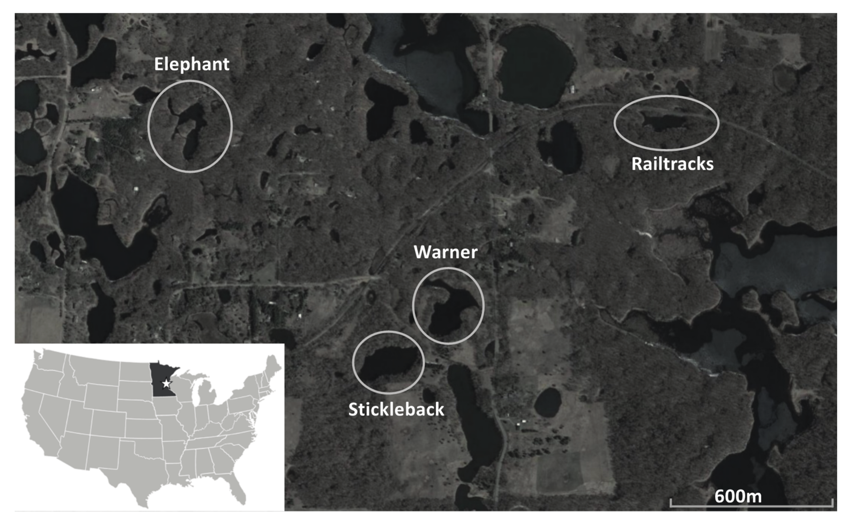
2.1. Pond Location

We sampled four ponds in east-central Minnesota, USA (Figure 1). Three of the ponds (Stickleback, Warner and Railtracks) had significant amounts of grass/shrub in their watersheds which, until the early 1970s, was in agriculture. The fourth pond (Elephant) had more deciduous tree cover in its watershed, although in the 1970s and 1980s more housing was constructed, and thus it is now in a low-density suburban area. There are no point–source discharges into the ponds and these ponds are isolated kettle ponds in confined watersheds with no inflowing/outflowing streams, so human influence (beyond the relatively undisturbed small watersheds that they are in) is minimal.

One pond (Stickleback) had brook stickleback (Culaea inconstans) introduced in 2013. By 2015–2016 the population of fish had increased and the pond shifted from one with a significant population of floating-leaved macrophytes to one dominated by phytoplankton and submerged macrophytes (personal communication, Ron Lawrenz, Director of the Lee & Rose Warner Nature Center). The few floating-leaved macrophytes in this pond were yellow waterlily (Nuphar variegata) and the submerged macrophytes were mainly stonewort (Char sp.), white-stem pondweed (Potamogeton praelongus), flat-stem pondweed (Potamogeton zosteriformis) and large-leaf pondweed (Potamogeton amplifolius). The other three ponds were fishless and contained varying amounts of floating-leaved and submerged macrophytes. Warner’s floating-leaved macrophytes were mainly white waterlily (Nymphaea odorata) with a few yellow water lilies. Railtracks also had mainly white waterlily and some coontail (Ceratophyllum demersum), while Elephant had mainly floating-leaf pondweed (Potamogeton natans) with a smaller amount of white waterlily.

We used ESRI ArcMap^® Version 10.6.1 to develop bathymetric maps of the ponds. We placed a 20 m × 20 m grid of points on the outline of the pond. At each point we measured the depth of the pond with a calibrated pole. We constructed a triangulated interpolated network (TIN) from the values and then used tools in ArcMap to create depth contours. The pond volume and area were also calculated from the TIN. We calculated the average depth of the pond as the volume/surface area.

2.2. Physical and Chemical Parameters

During the course of the ecosystem metabolism study (late May–late October 2018) we measured the conductivity of the ponds approximately every two weeks using a Hanna^® model HI98129 conductivity meter. These data were used to correct dissolved oxygen for salinity content and as a rough estimate of water quality in each pond. We tested whether there was a difference in conductivity between the ponds using a mixed model ANOVA with conductivity as the dependent variable, pond as the independent variable and date as the random variable. Tukey’s tests followed to examine paired differences between ponds. On two dates (June 13 and August 16, 2018) we sampled vertical profiles of dissolved oxygen, temperature and light. We measured light penetration using a Li-Cor^® model LI-193 4π underwater photosynthetic active radiation (PAR) sensor. From the linear regression between depth and ln(PAR) we calculated the extinction coefficient for each pond. Ponds with lower extinction coefficients have light penetrating farther into them. We measured dissolved oxygen and temperature with a YSI^® model 6600-M data sonde. To examine differences in these profiles, we conducted two-way ANCOVAs with pond and date as the independent variables, depth as the covariable and ln(PAR), dissolved oxygen or temperature as independent variables.

We measured nutrient levels in 2019, collecting bi-monthly water samples from May 30 through October 23. They were analyzed for total phosphorus (TP), total nitrogen (TN) and dissolved organic carbon (DOC) (water quality analysis was done by the St. Croix Watershed Research Station of the Science Museum of Minnesota). For DOC, samples were filtered through 0.4 µm PCTE membrane filters, were subjected to UV/persulfate digestion and then nondispersive infrared detection via a Teledyne Tekmar Phoenix^® 8000. For TP and TN, samples were subjected to a dual alkaline/persulfate digestion [38]. They were then analyzed for TP and TN with a SmartChem^® 170 water analyzer. We assessed whether there were differences in the TP, TN or DOC among ponds using a mixed-model ANOVA with the TP, TN or DOC as the dependent variable, pond as the independent variable and date as the random variable. This test was followed by a Tukey’s post hoc test to examine which ponds were significantly different.

From 17 May 2018 to 29 October 2018, we measured water temperature every 10 min just below the surface of the ponds using a HOBO^® Model U26-001 probe. We assessed whether there were differences in the mean water temperature and the range of temperatures experienced by the ponds on a daily basis. We used a mixed-model ANOVA with the water temperature or the range of temperatures as the dependent variable, pond as the independent variable and date as the random variable followed by a Tukey’s post hoc test to examine whether the temperatures and daily ranges varied among the ponds.

2.3. Pond Primary Production

To assess the density of macrophytes in the ponds we used a point-intercept method [39] at the points where depth measurements were taken. We made both qualitative and quantitative assessments of macrophyte abundance in late July. We visually assessed floating-leaved macrophytes and classified abundance into one of 5 categories (none, trace, sparse, medium or dense) at the grid of points at a 20 m × 20 m scale. The submerged macrophyte abundance was assessed using the spinning rake method [39]. We made qualitative assessment of submerged macrophytes visually in the same way as the floating-leaved macrophytes. Maps of the distribution of floating-leaved and submerged macrophyte abundances were constructed with ESRI ArcMap^® using a nearest neighbor interpolation between the points sampled. We calculated the percentage of the ponds’ areas represented by each abundance category from the maps.

In addition to a qualitative assessment of macrophyte abundance, we made a quantitative assessment of total macrophyte biomass (submerged and floating-leaved) using plants harvested with the rake. The rake was double headed and was 41.6 cm in length. The rake was rotated to remove a circular area of macrophytes (0.136 m² area). We air dried the macrophytes for > 48 h at 65 °C and weighed them to the nearest 0.1 g. We calculated macrophyte biomass per m² as the weight divided by the area taken by the rake sample. Maps of the distribution of biomass were constructed with ESRI ArcMap^® using nearest neighbor interpolation between values at the points sampled. From these data we calculated the average macrophyte biomass per m² by using the predicted biomass for each cell in the raster maps created from the nearest neighborhood interpolation. We estimated the total biomass for each pond by summing the average predicted biomass for all cells. Differences in macrophyte biomass among ponds was assessed by conducting a mixed-model ANOVA with the macrophyte biomass as the dependent variable, pond as the independent variable and date as the random variable.

To assess algal biomass, we took water samples from each pond approximately every 2 weeks during 2018. Water was filtered through Whatman^® GF/F glass fiber filters and frozen. We measured the chlorophyll a content by extracting in 90% acetone and measuring with an Aquaflour^® Model 8000 Fluorometer using EPA Method 445.0 [40]. From these data we were able to calculate the biomass of phytoplankton as µg chlorophyll a per L. Differences in phytoplankton biomass among ponds was assessed by conducting a mixed-model ANOVA with the amount of chlorophyll a as the dependent variable, pond as the independent variable and date as the random variable.

2.4. Pond Dissolved Oxygen Levels and Ecosystem Metabolism

From 17 May 2018 to 29 October 2018 (except in Warner when our instrument failed after 27 September 2018), we measured O₂ concentration every 10 min in each pond using HOBO^® Model U26-001 optical dissolved oxygen sensors fitted with copper antifouling guards. Oxygen sensors were placed in the center of the pond and maintained at 10 cm below the water surface. In Stickleback and Warner ponds we placed a second sensor at 0.75 m in depth (approximately halfway to the bottom of the ponds) starting on 22 June 2018, to examine vertical variability in O₂ levels. We also deployed HOBO^® weather stations at each pond. These weather stations were outfitted with photosynthetically active radiation (PAR) (HOBO^® Model S-LIA-M003), wind speed (HOBO^® Model S-WSB-M003) and barometric pressure sensors (HOBO^® Model BPB-CM50). Finally, we placed water depth sensors (HOBO^® model U20 L-04) in each pond. We compared the differences in O₂ level (arcsine-transformed% saturation) of the surface located sensors among ponds over the course of the sampling period using a mixed-model ANOVA with O₂ as the dependent variable, pond as the independent variable and date as the random variable. Tukey’s tests were conducted to examine which ponds were significantly different. We also compared the O₂ level of the surface and 0.75 m deep sensors in Stickleback and Warner ponds, again using a mixed model ANOVA followed by a Tukey’s test.

The components of ecosystem metabolism include gross primary production (GPP), respiration (R) and net ecosystem production (NEP = GPP − R). While some authors prefer to use net aquatic production (NAP) rather than NEP since emergent macrophytes and floating-leaved macrophytes would not contribute to estimates of primary production [37,41], we have continued to use the NEP terminology which is more widely used. Daily changes in GPP and R in aquatic systems can be estimated by daily changes in O₂ [42]. If R is constant throughout the day and GPP only occurs during daylight hours, then the differences in oxygen levels between daylight and night hours can be used to estimate R and GPP. Taking O₂ measurements throughout the day allows the components of ecosystem metabolism to be estimated as:

$$\frac{dC}{dt}=GPP-R+k\left(C_s-C\right)+GWA$$

NEP = GPP − R

where, C = concentration of oxygen, Cs = concentration of oxygen at saturation, k = reaeration coefficient and GWA = oxygen accrual from groundwater. The reaeration coefficient allows for the computation of O₂ changes due to the exchange of O₂ between the atmosphere and the water.

We made calculations of daily values of GPP, R and NEP using the R-script LakeMetabolizer [43]. The R-script provides estimates based on five different models of fitting the oxygen, light and temperature data collected (bookkeeping, Bayesian, Kalman, maximum likelihood estimation and ordinary least squares). It also provides the possibility of calculating each model using different methods of estimating the reaeration coefficient. With the data we collected we were able to estimate the reaeration coefficient with three different methods—Cole and Caraco [44], Crusius and Wanninkhof [45] and Vachon and Prairie [46]. Winslow et al. [43] details the assumptions behind both the different models and reaeration coefficients. We were able to generate 15 estimates of daily GPP, R and NEP (5 models with 3 estimates of reaeration coefficients each). Winslow et al. [43] did not provide information on the best model to use. They did comment on the issues surrounding the models providing “impossible” values, i.e., values where GPP < 0 or R > 0, both of which are biologically unreasonable. We examined whether there were differences in the proportion of values that were “impossible” among ponds in the model–reaeration coefficient groups using nominal logistic regression, with the proportion of metabolism values that were “impossible” as the dependent variable, and with pond and the combined model–reaeration coefficients groups and their interaction as independent variables. We decided to use the combination of model and reaeration coefficient that gave the fewest “impossible” values for our further examination of the values of ecosystem metabolism.

Once we calculated daily values of GPP, R and NEP using our chosen model and reaeration coefficient, we compared these values among ponds based on the surface located sensors using mixed-model ANOVA with the GPP, R or NEP as the dependent variables, pond as the independent variable and date as the random variable. We tested whether these values were from normal distributions, and since they were, we did not transform the data. We examined which ponds were significantly different using a post hoc Tukey’s test. We examined whether there was a correlation between GPP and R in the ponds using an ANCOVA with R as the dependent variable, pond as the independent variable and GPP as the covariable, followed by a Tukey’s test to examine which ponds were significantly different from one another. We also examined the impact of temperature and light intensity (PAR) on GPP, R and NEP. We used ANCOVAs, with pond as the independent variable and either average daily temperature (log₁₀-transformed) or total daily light intensity as covariables and GPP, R and NEP as independent variables. Again, we used post hoc Tukey’s tests to examine which ponds were significantly different and t-tests to compare slopes.

To examine the impact of vertical location of the sensors on our estimates of ecosystem metabolism, for the two ponds where we had oxygen probes deployed at both the surface and 0.75 m below the surface, we used a mixed-model ANOVA with GPP, R or NEP as the dependent variable, pond as the independent variable and date as the random variable.

2.5. Statistics

All statistical analyses were carried out with JMP^® Pro Version 14.2 (SAS Institute, Inc., Cary, NC, USA).

3. Results

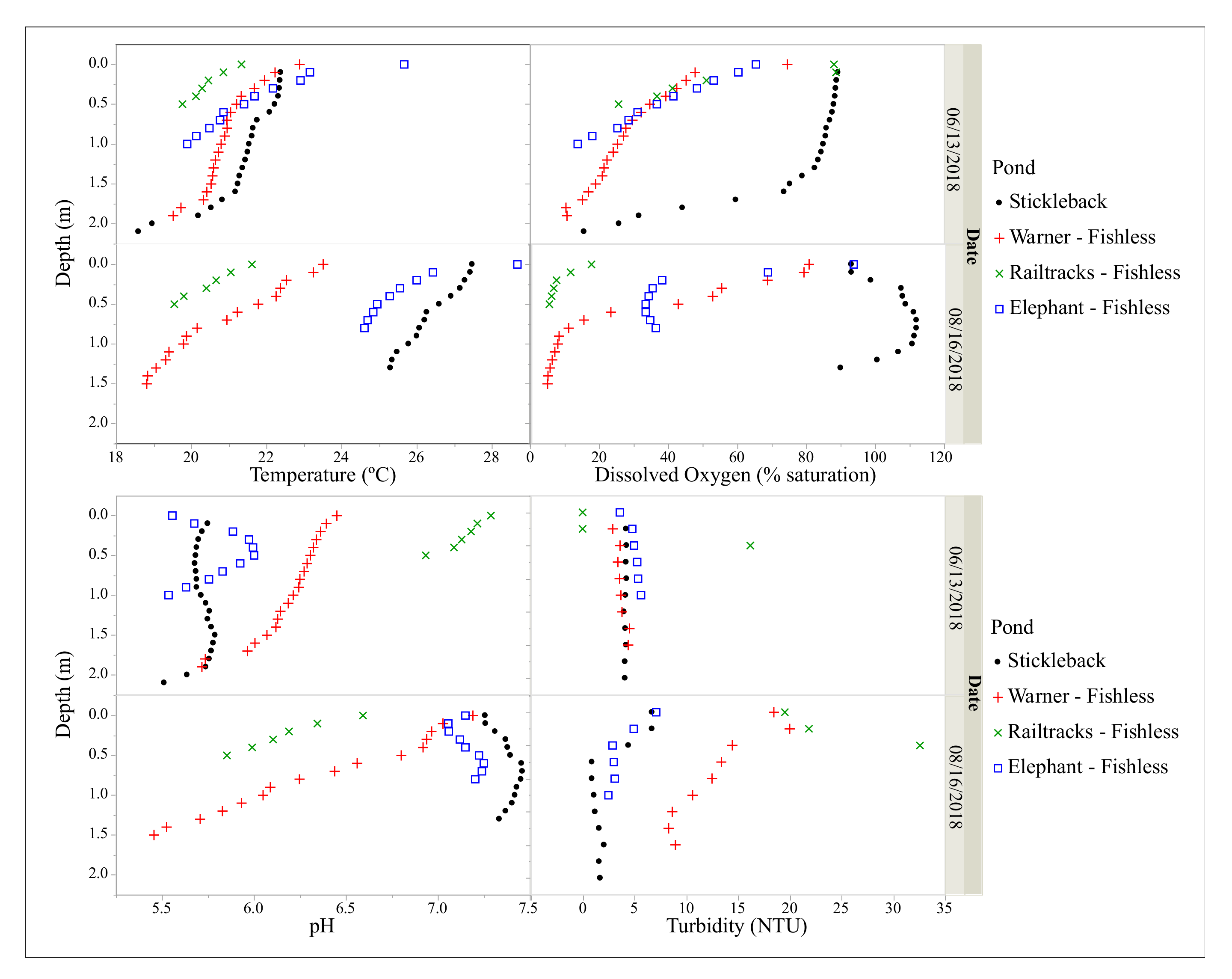
3.1. Physical and Chemical Parameters

For the two dates (mid-June and mid-August) when we measured vertical profiles in the ponds, we found that Stickleback and Elephant had the greatest light penetration, while Railtracks had the lowest light penetration (

Table 1. Values for various physical and chemical parameters for four ponds in east-central Minnesota. Within parameters, values with the same letter are not significantly different from one another (Tukey’s post hoc test). Cells labeled in bold show the pond with the maximum value of a parameter, while those in italics show the pond with the minimum value.

Parameter	Pond
	Stickleback	Warner	Railtracks	Elephant
Average depth (m)	1.5	1.2	0.47	0.57
Pond surface area (m2)	15,121	16,812	6995	7077
Pond volume (m3)	22,733	19,806	3301	7077
Conductivity (µS/cm) 1	40.1 a (4.0)	70.0 (7.7) b	23.3 (11.2)c	30.4 a,c (3.7)
Extinction coefficient—June 13, 2018 (r²)	2.33 (0.91)	2.72 (0.95)	6.96 (0.98)	2.96 (0.97)
Extinction coefficient—July 16, 2018 (r²)	2.14 (0.93)	3.99 (0.98)	6.39 (0.94)	2.56 (0.96)
Total phosphorus (µg/L) 2,4	89.4 (9.3) a	46.5 (9.3) b	44.7 (9.3)b	56.5 (9.3) a,b
Total nitrogen (mg/L) 2,4	1.6 (0.2) a	0.7 (0.2)b	0.7 (0.2)b	0.8 (0.2) b
Dissolved organic carbon (mg/L) 2,4	9.8 (0.5) a	6.2 (0.5)b	6.7 (0.5)b	7.6 (0.5) c
Water temperature (°C) 2,3	21.3 (0.05) a	20.3 (0.05) b	20.1 (0.05)c	20.7 (0.05) d
Average daily water temperature range (°C) 2,3	5.1 (0.23)a	7.0 (0.23) b	8.0 (0.23) c	6.8 (0.23) b
Mean dissolved oxygen saturation (%) 2,3	90.6 (0.19) a	31.0 (0.20)b	35.2 (0.19) c	58.9 (0.19) d

¹ Value is mean and number in parenthesis is standard deviation. ² Value is least squares mean and number in parenthesis is standard error. ³ Values are for surface measurements throughout the research period and do not include data obtained at 0.75 m. ⁴ Values are from 2019 while all other values are from 2018.

). Two-way ANCOVAs indicated that water depth, pond and date and their interactions significantly influenced light penetration (

Table 2. ANCOVA results (F-value, degrees of freedom and probability) for effects of water depth, pond and date of analysis of depth profiles of photosynthetic active radiation (PAR), temperature and dissolved oxygen.

Independent Variables	PAR 1 (µmoles/m2/sec) 2	Temperature (°C) 2	Dissolved Oxygen 3 (% Saturation) 2
Pond	64.1; 3, 50; < 0.0001	320; 3, 102; < 0.0001	108.8; 3, 92; < 0.0001
Date	22.1; 1, 50; < 0.0001	87.1; 1, 102; < 0.0001	0.1; 1, 92; 0.8
Depth	471.9; 1, 50; < 0.0001	232.3; 1, 102; < 0.0001	104.9; 1, 92; < 0.0001
Pond × Date	24.0; 3, 50; < 0.0001	195.5; 3, 102; <0.0001	9.0; 3, 92; < 0.0001
Date × Depth	0.1; 1, 50; 0.7	3.6; 1, 102; 0.06	4.6; 1, 92; 0.04
Pond × Date × Depth	3.4; 3, 50; 0.03	9.2; 3, 102; < 0.0001	12.7; 3, 92; < 0.0001

¹ Analysis completed on ln(PAR). ² First value is F-value, next are degrees of freedom and the third is the probability. ³ Analysis completed on arcsine square root transform of % saturation.

). An ANCOVA indicated that depth, date, pond and their interactions significantly influenced temperature (Table 2). Temperature profiles from these dates indicated that there was some stratification in all of the ponds, but it was most pronounced during the August sampling period (Figure 2). The temperature in Stickleback and Elephant increased more over the period (mid-June–mid-August) than the other two ponds. Similarly, the dissolved oxygen profile showed some level of stratification in all ponds. ANCOVA showed that depth, date, pond and their interactions were significant in most cases (Table 2). Oxygen levels (as% saturation) were highest in Stickleback and Elephant and lowest in Warner (Figure 2).

Over the entire study period there were significant differences in the average water temperature among ponds (mixed model ANOVA—F_3,67077 = 10,810.0, p < 0.0001) with Stickleback having the highest average temperature and Railtracks the lowest average temperature (Table 1). The range of temperatures experienced on a daily basis varied among the ponds (ANOVA—F_3,463.2 = 64.2, p < 0.0001). A Tukey post hoc test indicated the temperature range was not significantly different between Warner and Elephant, but all other paired comparisons were statistically significant (Table 1). Stickleback had the lowest range of temperatures among the ponds and Railtracks had the highest temperature variation.

There were also significant differences among the ponds in the levels of total phosphorus (mixed model ANOVA F_3,21 = 5.3, p = 0.0073), total nitrogen (mixed model ANOVA—F_3,21 = 9.6, p = 0.0004) and DOC (mixed model ANOVA—F_3,21 = 46.6, p < 0.0001) (Table 1). All three nutrients were highest in Stickleback, with total phosphorus and nitrogen lowest in Railtracks and DOC lowest in Warner. There were significant differences in the conductivity of the ponds (ANOVA—F_3,18 = 64.5, p < 0.0001) with Warner having the highest conductivity and Railtracks having the lowest conductivity (Table 1).

3.2. Primary Production

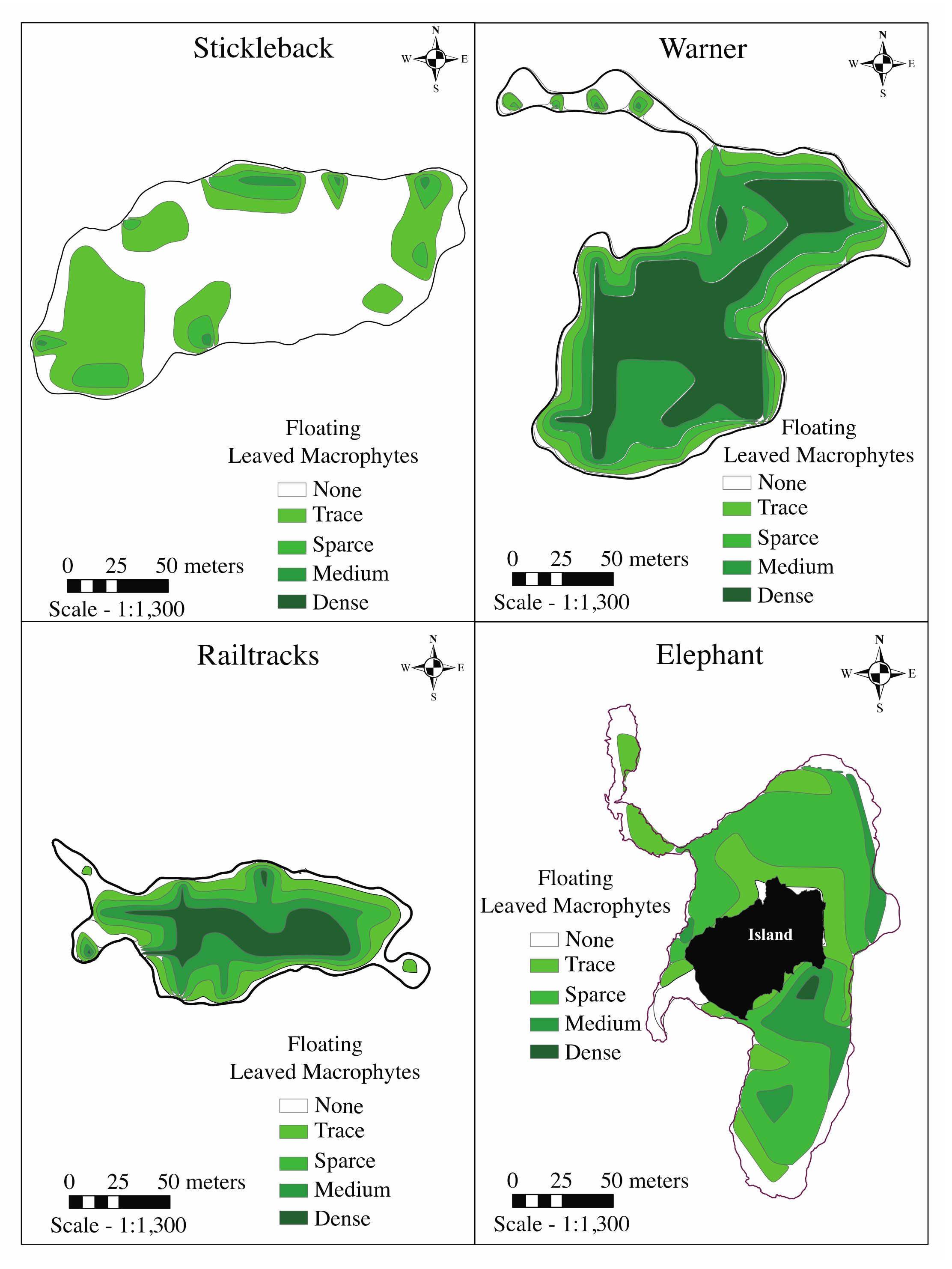
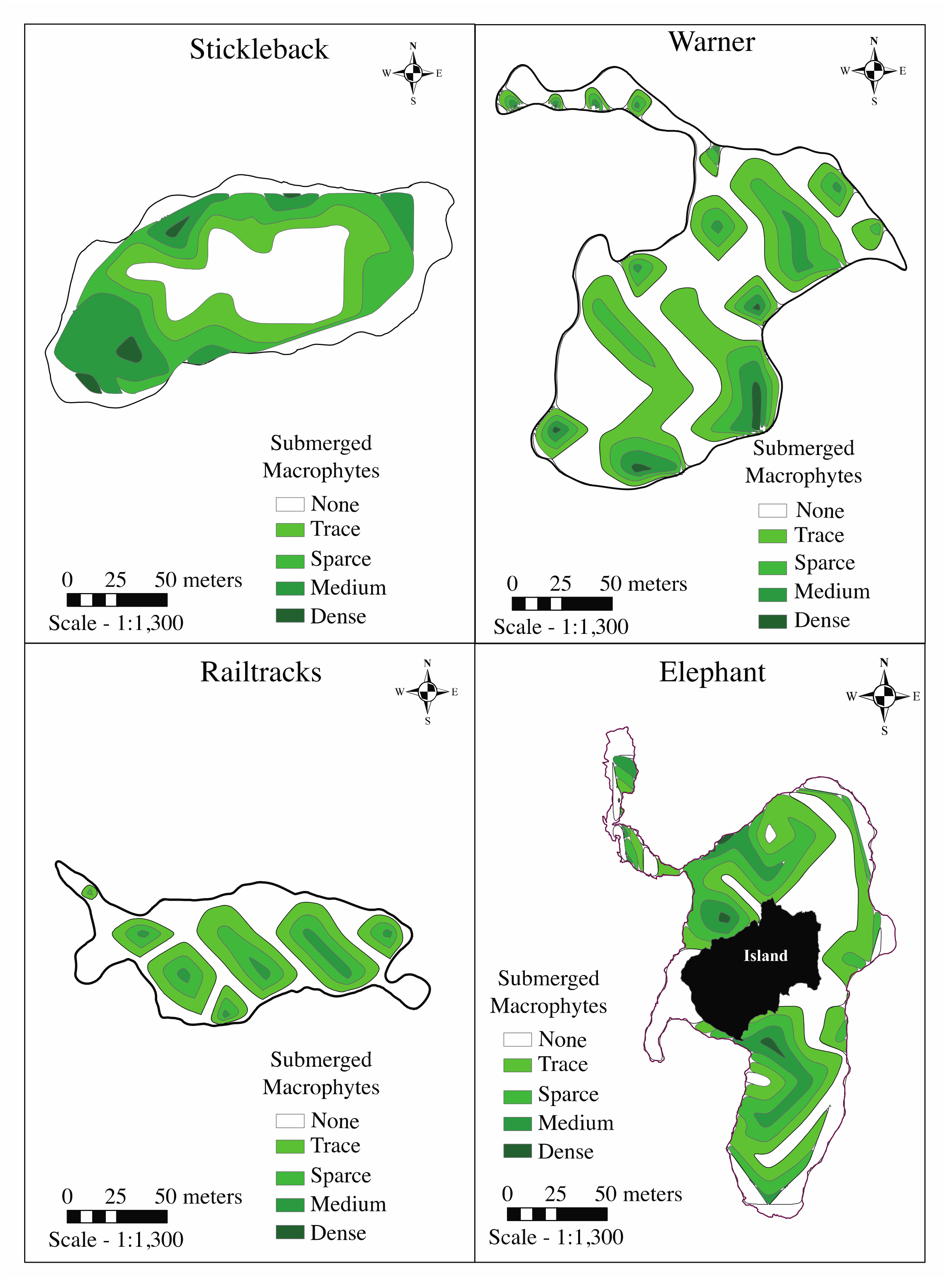
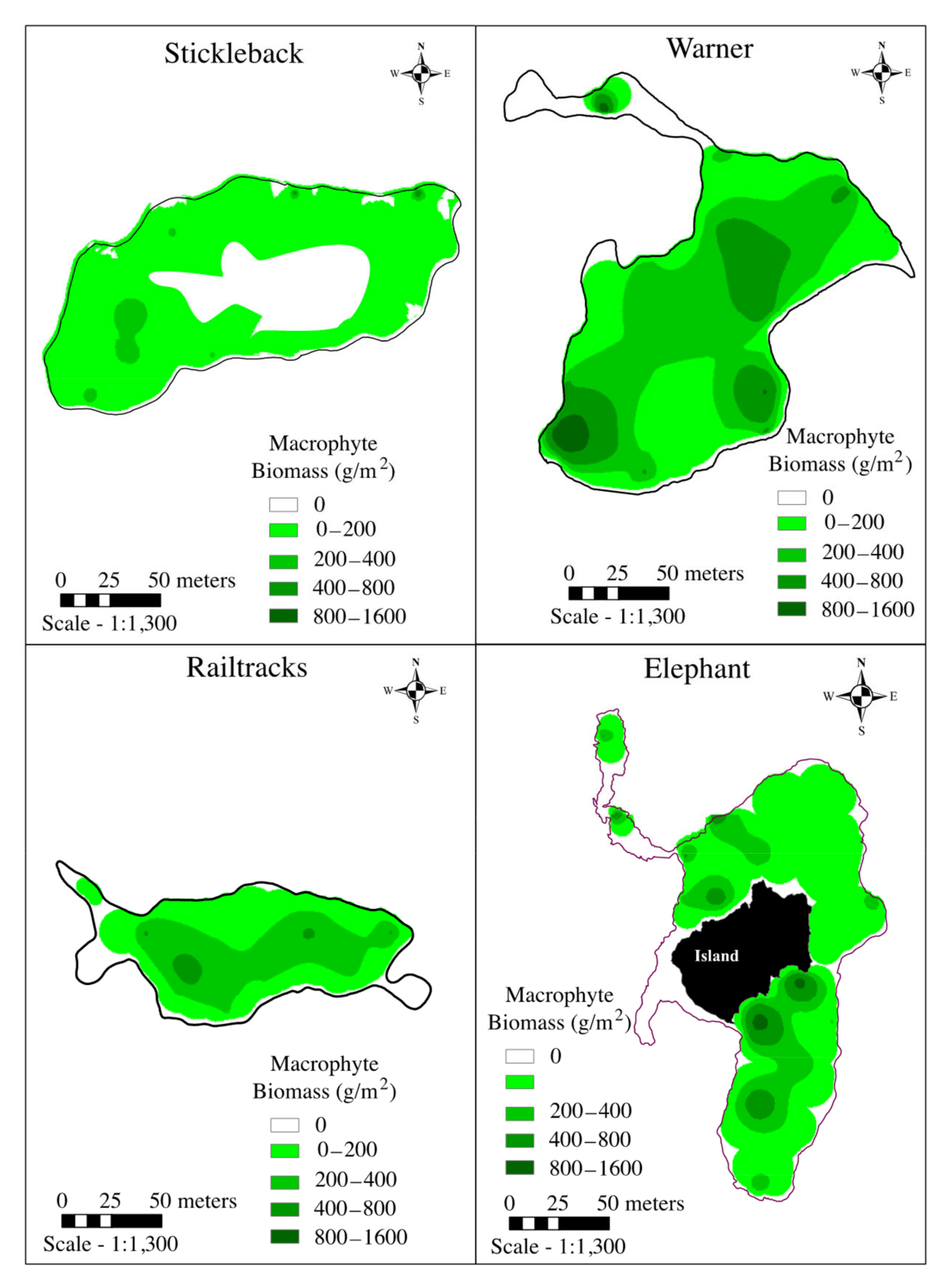
3.2.1. Macrophyte Abundance

Figure 3 and Figure 4 show the distribution of floating-leaved and submerged macrophytes in the four ponds. Warner had a large percentage of its surface covered by floating-leaved macrophytes by the end of July, while Stickleback had much less of its surface covered compared to the other ponds (

Table 3. Amounts of various primary producers (macrophytes and phytoplankton) and ecosystem metabolism measures (GPP—Gross Primary Production, R—Respiration and NEP—Net Ecosystem Production) from four ponds in east-central Minnesota. Within parameters, values with the same letter are not significantly different from one another (Tukey’s post hoc test). Cells labeled in bold show the pond with the maximum value of a parameter, while those in italics show the pond with the minimum value.

Parameter	Pond
	Stickleback	Warner	Railtracks	Elephant
Submerged macrophytes (% medium or dense coverage)	20.7	6.1	3.3	8.4
Floating-leaved macrophytes (% medium or dense coverage)	0.9	61.2	43.7	12.4
Total macrophyte biomass (kg)	376.5	4129.2	1166.5	1487.5
Average macrophyte biomass (g/m2) 1	24.9 (36.4)a	229.3 (3186.9) b	151.6 (117.3) c	98.6 (141.7) d
Phytoplankton biomass (µg chl a/L) 2	5.34 (1.17) a	2.6 (1.2)a	6.65 (1.3) a,b	9.3 (1.2) b
Mean GPP (mgO2/L/day) 1	3.2 (2.3) a	2.2 (2.2)b	4.3 (4.0) c	5.5 (4.0) d
Mean R (mgO2/L/day) 1	−3.6 (2.7)a	−3.7 (3.4) a	−4.4 (4.9) a	−6.8 (6.1) b
Mean NEP (mgO2/L/day) 1	−0.4 (1.8) a	−1.5 (2.4)b	−0.1 (2.6) a	−1.3 (3.3) b

¹ Value is mean and number in parenthesis is standard deviation. ² Value is least squares mean and number in parenthesis is standard error.

). Stickleback had the largest coverage of submerged macrophytes (Table 3). There was a significant difference among ponds in the actual biomass of macrophytes (Figure 5, ANOVA—F_3,257743 = 29,461, p < 0.0001) with Stickleback having the lowest levels of macrophyte biomass both in terms of average macrophyte biomass per square meter and total biomass for the pond, while Warner had the highest macrophyte biomass per square meter and total biomass for the whole pond (Table 3).

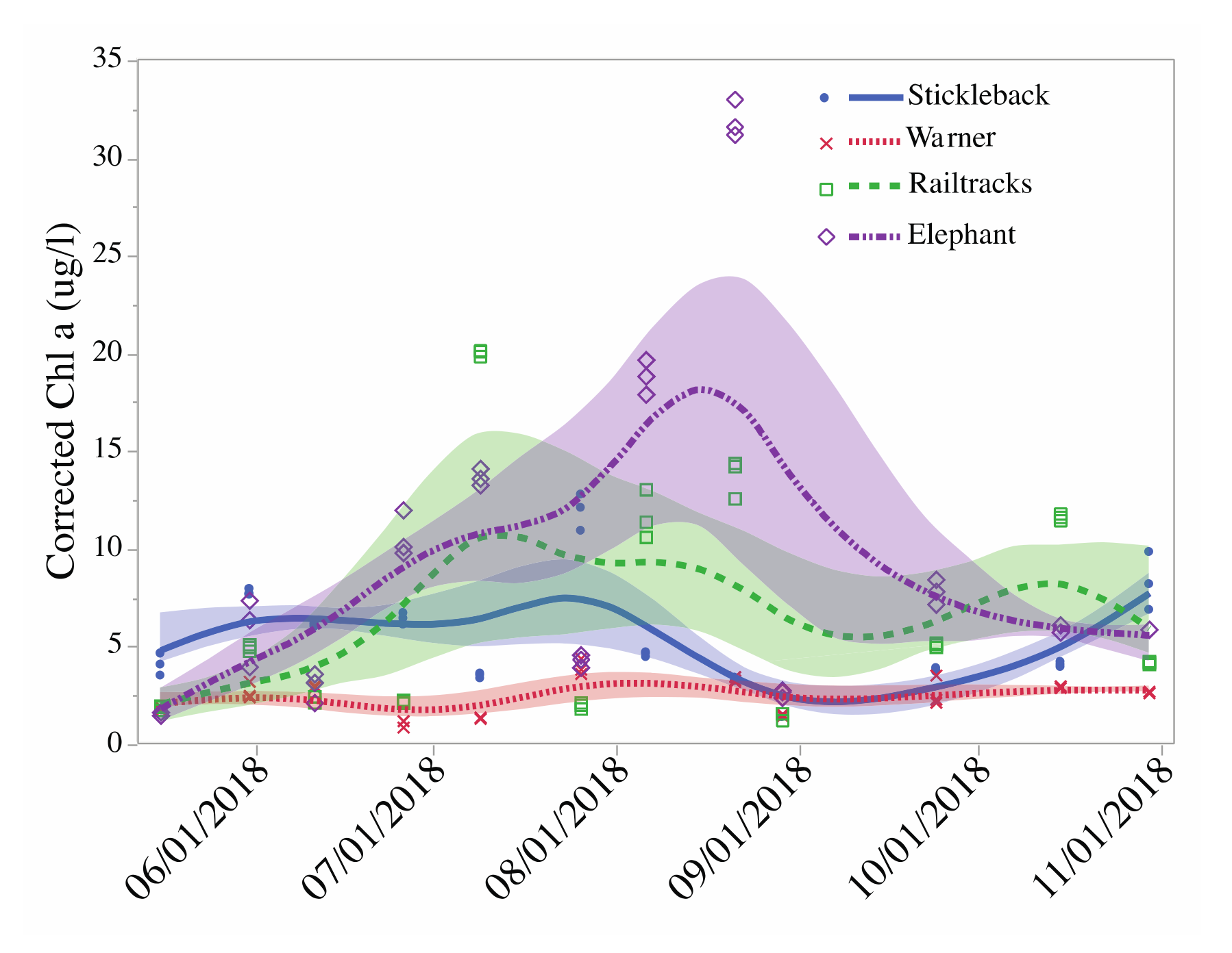
3.2.2. Phytoplankton

Phytoplankton biomass varied across the seasons and between ponds (Figure 6). A mixed model ANOVA indicated there were significant differences among ponds (F_3,125 = 12.5, p < 0.0001). A post hoc pairwise Tukey’s test indicated that Elephant pond had higher average phytoplankton biomass than all of the other ponds, and this difference was significant for all ponds except Railtracks. Warner had the lowest phytoplankton biomass, although there was a good deal of overlap with all of the ponds except Elephant (Table 3).

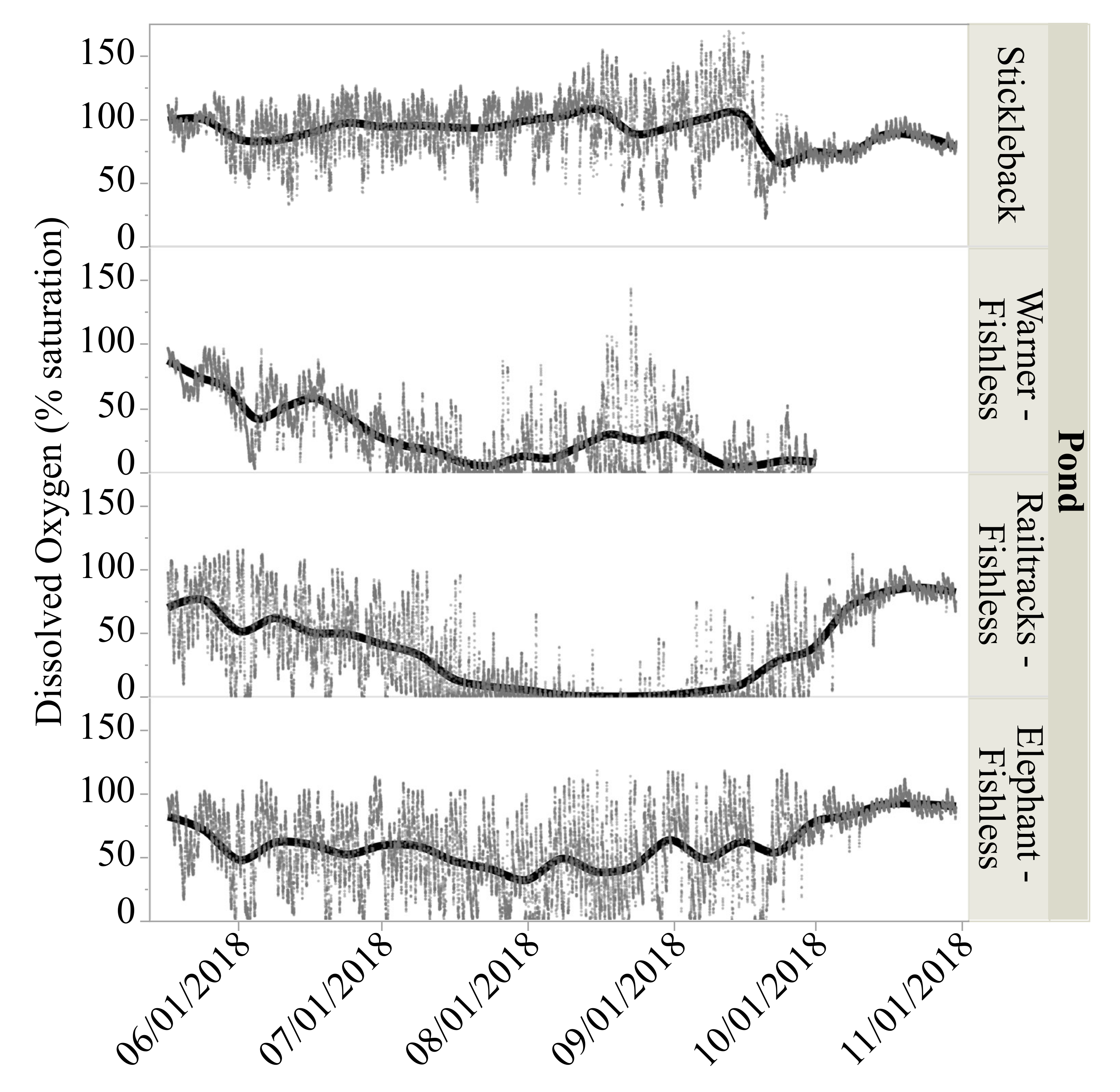
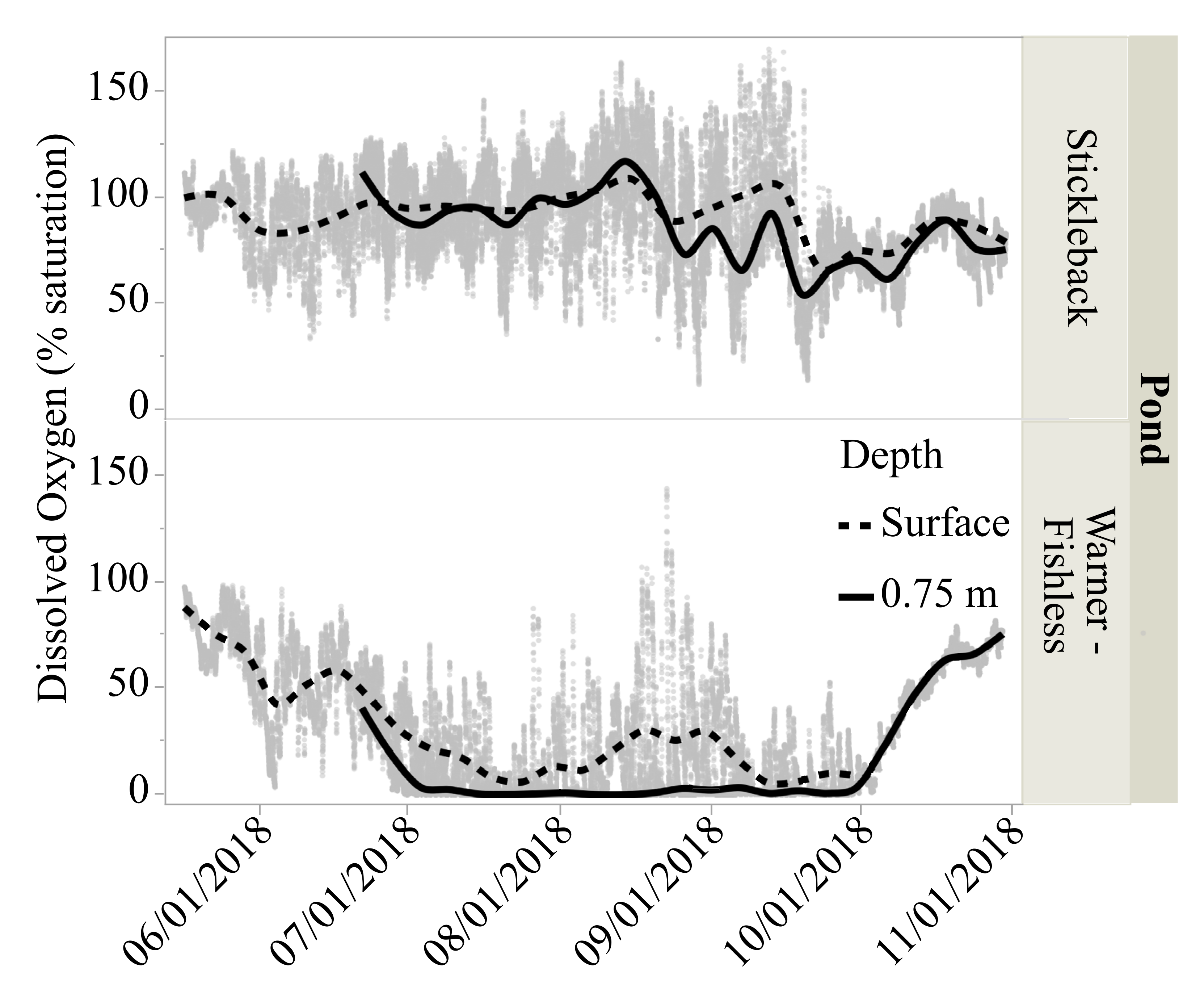
3.3. Dissolved Oxygen Levels

The surface water dissolved oxygen levels measured throughout the season varied among ponds (Figure 7) and were significantly different from one another (F_3,60695 = 23,125.8, p < 0.0001; Table 1-note: the surface probe in Warner failed on Sept 28 and thus data were not available for October). On average, Stickleback had the highest dissolved oxygen levels and Warner had the lowest oxygen levels (Table 1).

In both Stickleback and Warner, we measured it at a depth of 0.75 m in addition to measuring dissolved oxygen at the surface (Figure 8). For Stickleback, the mean at the surface over the sampling period was 90.7% (std. deviation = 20.4), while it was 85% (std. deviation = 22.5) at 0.75 m. A mixed model ANOVA indicated this difference was significant (F_1,20668 = 2420.5, p < 0.0001). For Warner, the mean oxygen was 28.5% (std. deviation = 27.7) at the surface and 13.0% (std. deviation = 22.8) at 0.75 m. A similar mixed model ANOVA indicated a significant difference in oxygen level between depths (F_1,8643 = 16.7, p < 0.0001). Despite differences in the oxygen levels between depths in both ponds, for Stickleback the coefficients of variation (variance/mean) were more similar among depths (surface: 22.5%; 0.75 m—26.5%) and smaller than the coefficients of variation in Warner (surface: 96.9%; 0.75 m—175.2%).

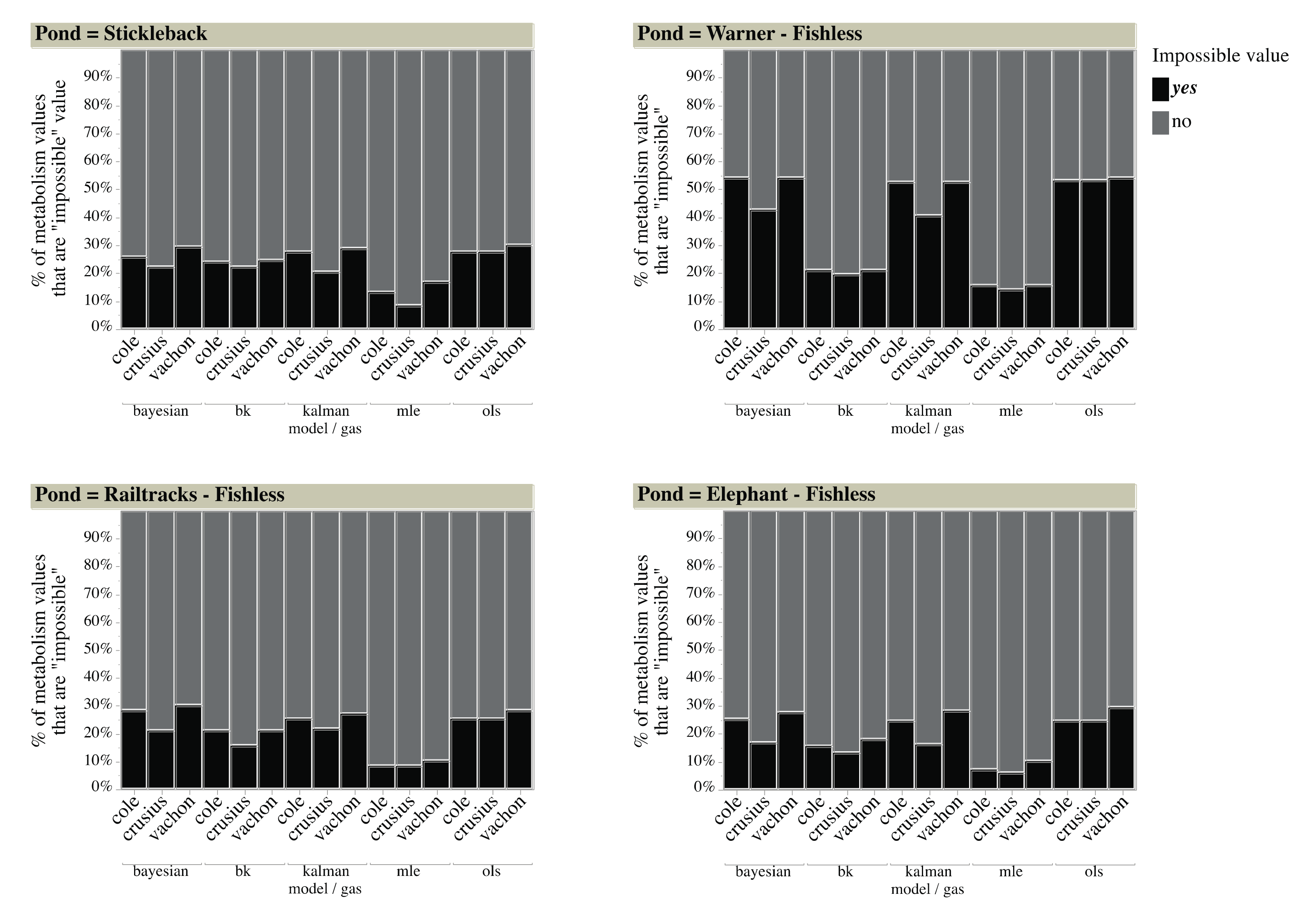
3.4. Pond Metabolism—Model Selection

We calculated GPP, R and NEP using a combination of 5 possible models and 3 estimates of the reaeration coefficient, giving a total of 15 estimates for each of these factors. Figure 9 shows the range of so-called impossible measures that were calculated from these estimates from the measurements made at the surface of the ponds. Impossible measures include GPP < 0 and R > 0. A nominal logistic regression showed that the proportion of metabolism values that were “impossible” were significantly different between ponds, in addition to the combined model–reaeration coefficient groups and their interaction (Figure 9, pond: $x_3^2$ = 174.6, p < 0.0001; model–reaeration coefficient: $x_{14}^2$ = 414.6, p < 0.0001; pond*model–reaeration coefficient: $x_{42}^2$ = 68.7, p = 0.006). Regardless of pond, the maximum likelihood estimate (mle) model coupled with the Crusius and Wanninkhof [45] method of estimating the reaeration coefficient gave the fewest number of “impossible” values (range: 6.1–14.3%) (Figure 9). Consequently, all analyses of differences in GPP, R and NEP among and within ponds and in those factors that may influence these parameters were based on the maximum likelihood estimate model using the Crusius and Wanninkhof [45] reaeration coefficient. With this model and reaeration coefficient the ponds had “impossible” values of 6.1%, 8.5%, 8.5% and 14.3% for Elephant, Stickleback, Railtracks and Warner, respectively. Our values of the reaeration coefficient (k₆₀₀) ranged from 0.04–1.2 m/day. While there were significant differences among ponds (ANOVA F_3,95958 = 586.9, p < 0.0001), the difference in the averages were quite small (0.045–0.055) and the large sample size may account for the significance.

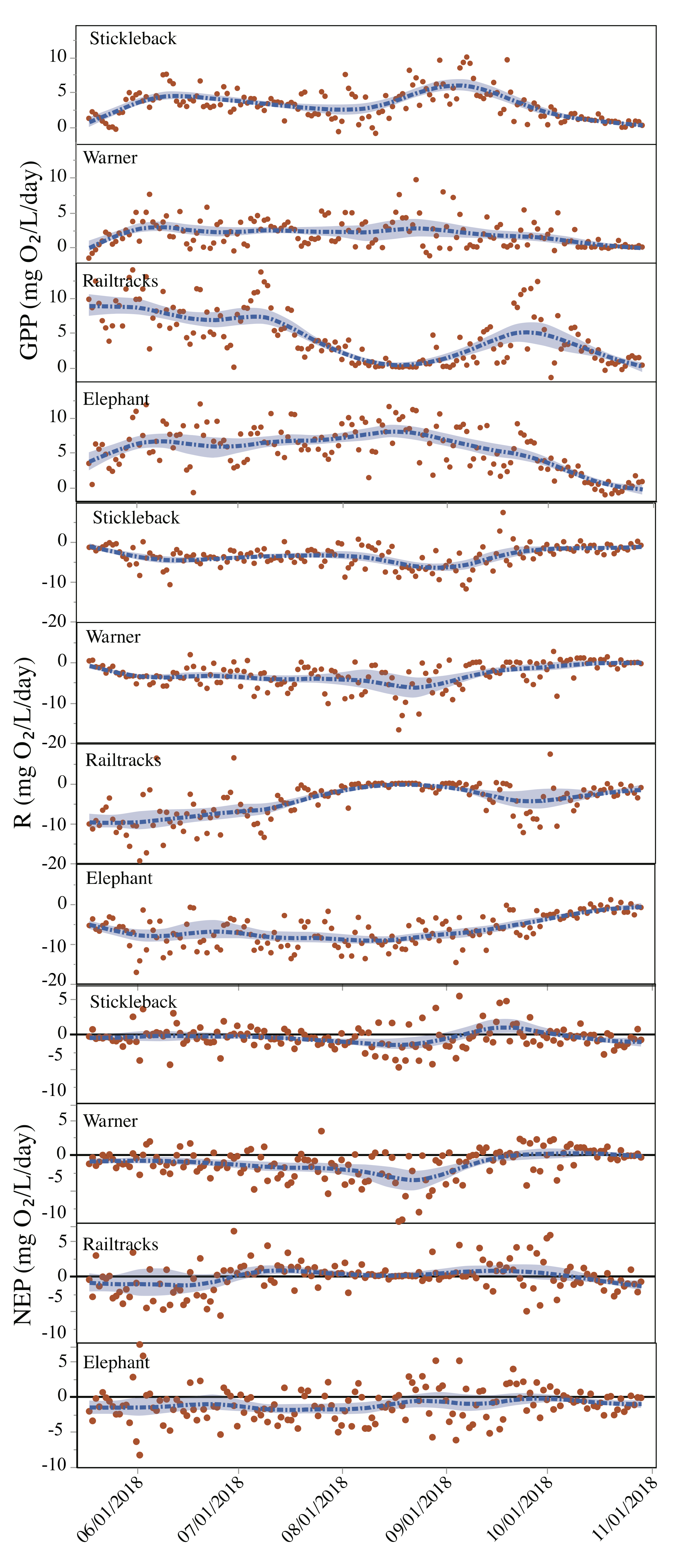
3.5. Pond Metabolism—Variation between Ponds and Depths

Figure 10 shows the seasonal changes in GPP, R and NEP among the ponds. Using mixed model ANOVAs we found significant differences among the ponds for the various components of ecosystem metabolism (GPP: F_3,455.2 = 41.5, p < 0.0001; R: F_3,464.6 = 21.0, p < 0.0001; NEP: F_3,472.4 = 13.6, p < 0.0001). GPP for all of ponds were significantly different from one another with Elephant having the highest average GPP and Warner having the lowest average GPP (Table 3). R in Elephant was significantly greater (values were more negative) than the other ponds (Table 3). R values in the other ponds did not differ significantly from one another (Table 3). NEP was highest in Warner and Elephant and lowest in Stickleback and Railtracks (Table 3). On average, all ponds were heterotrophic (R > GPP (Table 3)), although there were a number of days when the ponds were autotrophic (NEP > 0; 32%, 27%, 48% and 28% of the days for Stickleback, Warner, Railtracks and Elephant, respectively (Figure 10)).

We found that there was a correlation between R and GPP and that these relationships varied by pond (Pond: F_3,627 = 15.2, p < 0.0001; GPP; F_1,627 = 1022.8.3, p < 0.0001; Pond × GPP: F_3,627 = 10.7, p < 0.001). The slope of the relationships was greatest for Warner and lowest for Stickleback, and the difference was significant (t₆₂₀ = 5.5, p < 0.0001). The slope for Stickleback was not significantly different from the other two ponds.

For the two ponds where we had oxygen probes deployed at the surface and 0.75 m below the surface, Stickleback had significant differences in R and NEP, but not GPP between the depths (mixed model ANOVAs, GPP: F_1,153.5 = 2.9, p = 0.09; R: F_1,161.5 = 17.1, p < 0.0001; NEP: F_1,161 = 22.5, p < 0.0001); in contrast, for Warner we found that GPP, R and NEP were significantly different between depths (mixed model ANOVAs, GPP: F_1,156.4 = 116.0, p < 0.0001; R: F_1,174.4 = 115.6, p < 0.0001; NEP: F_1,173 = 51.9, p < 0.0001). For Stickleback, surface measurements of GPP, R and NEP were higher than at 0.75 m (mean surface values for GPP, R and NEP: 3.2, −3.6 and −0.44 mgO₂/L/day; mean values at 0.75 m: 2.8, −2.2 and 0.57 mgO₂/L/day). These differences result in Stickleback being classified as heterotrophic based on surface measurements and autotrophic based on measurements at 0.75 m. For Warner, 58.9% of the values were “impossible” values (GPP < 0 and R > 0) making comparisons of average GPP and R between depths meaningless.

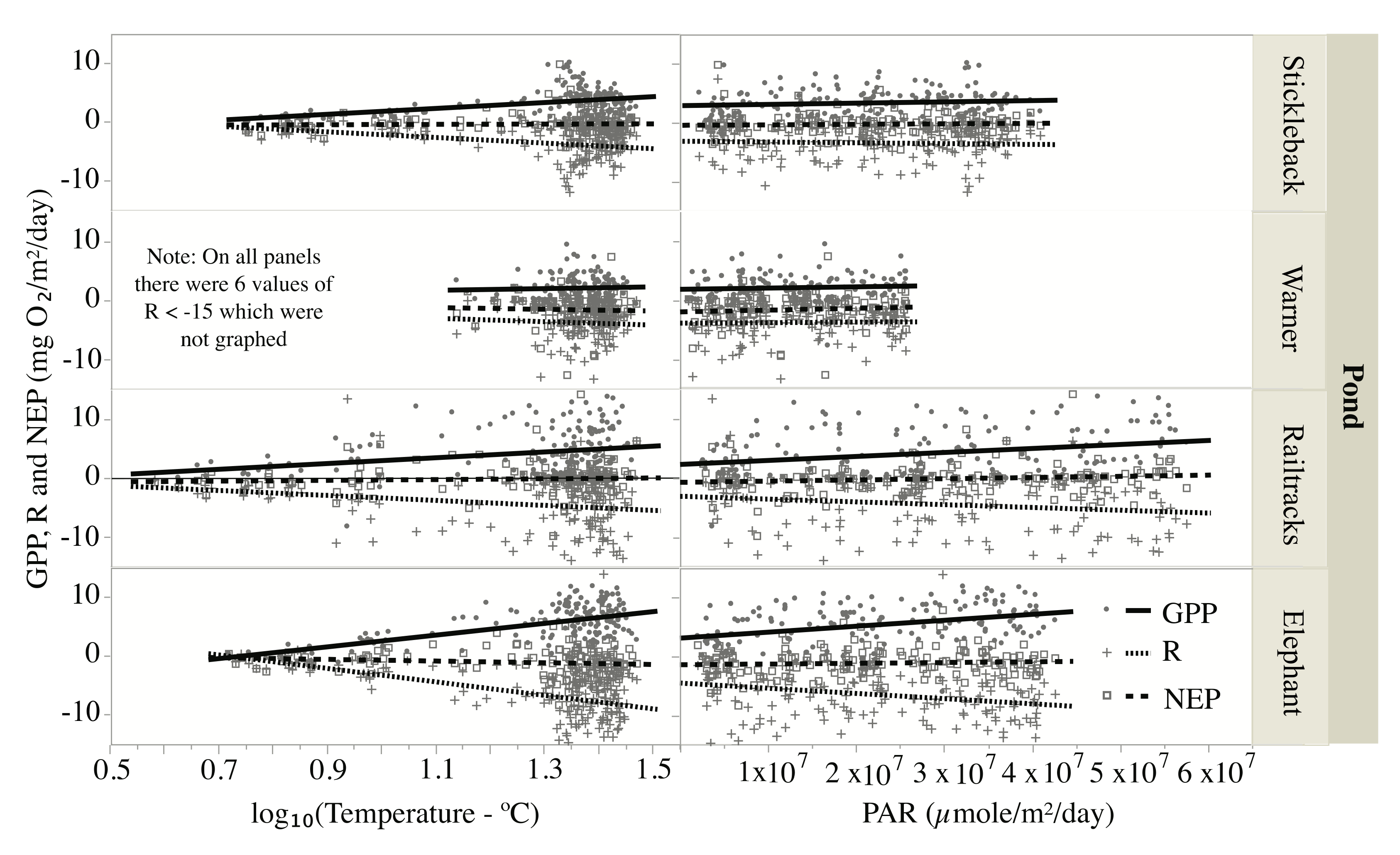
3.6. Pond Metabolism—Effects of Temperature and Light

ANCOVA indicated that pond, water temperature (log-transformed) and their interaction had significant impacts on GPP and R (

Table 4. ANCOVA results (F-value, degrees of freedom and probability) for effects of water temperature or light and pond on measures of ecosystem metabolism (GPP, R and NEP) for four ponds in east-central Minnesota, USA.

Category of Comparison	Independent Variables	Dependent Variable F; df; p
		GPP	R	NEP
Temperature	Pond	30.9; 3626; < 0.0001	21.6; 3, 626; < 0.0001	8.9; 3626; < 0.0001
	log10 (temperature °C)	23.0; 1626; < 0.0001	15.5; 1626; < 0.0001	0.3; 1626; 0.58
	Pond × Temperature	5.4; 3626; 0.001	5.4; 3626; 0.001	1.1; 3626; 0.34
Light	Pond	20.5; 3626; < 0.0001	17.6; 3626; < 0.0001	5.7; 3, 626; 0.0008
	PAR (µmoles/m2/sec)	19.7; 1626; < 0.0001	4.9; 1626; 0.027	3.7; 1626; 0.055
	Pond × Temperature	3.1; 3626; 0.026	1.8; 3626; 0.14	0.2; 3626; 0.88

). Both GPP and R increased with temperature (R becoming more negative) (Figure 11). There was no significant effect of temperature on NEP (Table 4). Pairwise comparisons of the slope of the temperature versus GPP or R showed that the slope of the temperature versus GPP relationship was significantly higher for Elephant than the other ponds (t₆₂₆ = 3.47, p = 0.0006) and was also higher (more negative) for R (t₆₂₆ = 3.12, p = 0.0019). No other pairwise comparisons were significant.

There was also a significant effect of PAR on GPP and R and a close to significant effect on NEP (Figure 11, Table 4). Again, pairwise comparisons of slopes of PAR versus GPP or R indicated that Elephant had a significantly higher slope than the other ponds for both GPP and R (GPP: t₆₂₆ = 2.68, p = 0.008; R: t₆₂₆ = 2.24, p = 0.02).

4. Discussion

4.1. Physical/Chemical/Biologic Conditions of the Ponds

All of the ponds in our study, regardless of the amount of floating-leaved macrophytes were relatively clear. The chlorophyll content for all ponds was within the typical range for lakes in the central hardwood area of Minnesota [47] and small ponds more generally [48]; however, they were all low compared to a large number of both small clear (< 20 µg/L) or turbid (> 31 µg/L) lakes in Minnesota [37,49]. Elephant was the only pond that had phytoplankton chlorophyll biomass levels > 31 µg/L, which Zimmer [49] considered turbid, and then only in late August. The pond with fish (Stickleback) historically had high levels of floating-leaved macrophytes similar to Warner. With the introduction of fish, a new state was established: one with few floating-leaved macrophytes, a reduction in amphipods and a shift in the Chaborous zooplankton assemblage (Ron Lawrenz, Warner Nature Center, personal communication, Emily Schilling, unpublished data). Stickleback are known to graze on zooplankton and can potentially bring about an increase in phytoplankton due to top-down control [50,51]. However, unlike other studies where the introduction of fish led to a loss of macrophytes and increased amounts of phytoplankton [24,25,26,27,29], Stickleback had the greatest percentage of submerged macrophytes and an intermediate level of phytoplankton compared to other ponds in our study. Stickleback also had the highest level of nutrients (P and N) which again would lead to an expectation of increased levels of phytoplankton and low amounts of both submerged and floating-leaved macrophytes. Horppila and Nurminen [52] indicated that rooted floating-leaved macrophytes lower P concentrations in the water column because of their high uptake of P through the roots resulting in lower sediment P concentrations. Hilt et al. [53] also pointed out rooted macrophytes may influence the level of nutrient retention in small ponds by allowing N and P to be stored in plant tissues. This process could account for the pond with the highest level of floating-leaved macrophytes (Warner) having among the lowest P levels, and the pond with lowest biomass of floating-leaved macrophytes and lowest overall macrophyte biomass (Stickleback) having the highest P levels. The differences in the amounts and types of macrophytes dominant in the ponds could be due to slight differences in the surrounding vegetation and land use (Elephant having higher amounts of housing and deciduous forest), the depth of the ponds (Railtracks much shallower than the others) and as mentioned above the presence of fish in Stickleback.

In June there was little difference in phytoplankton populations, as assessed through chlorophyll a, among ponds. As the summer progressed, chlorophyll a content remained low in the pond with the highest levels of floating-leaved macrophytes (Warner), while chlorophyll a content was higher in the other two ponds. Stickleback had intermediate levels of chlorophyll a. Light penetrated farther into the water column in Stickleback indicating that even though chlorophyll a level were intermediate, something other than light was controlling phytoplankton production. While Elephant had the highest average phytoplankton biomass, it had more floating-leaved macrophytes than Stickleback. The smaller size of the leaves of the floating-leaved macrophytes in Elephant (Potamogeton—leaf size length generally 5–10 cm, versus waterlily—leaf size length generally 7–40 cm) led to a fairly high level of light penetration into the pond (small extinction coefficient) and thus may be responsible for its fairly high level of chlorophyll a compared to the other ponds with greater amounts of floating-leaved macrophytes. However, this does not explain the higher amount of phytoplankton in Elephant than Stickleback. That Stickleback did not have the most phytoplankton of our study ponds is surprising, considering that it had the lowest amount of floating-leaved macrophytes and the highest P and N concentrations. The abundance of submerged macrophytes in Stickleback could be responsible for the reduced phytoplankton through a variety of mechanisms including allelopathic interactions, shading and providing shelter for zooplankton that can graze on the phytoplankton [54,55,56,57].

4.2. Ecosystem Metabolism

We calculated various components of ecosystem metabolism (GPP, R and NEP) and found that there were significant differences in all of these measures among the ponds. We calculated the values of GPP, R and NEP for a number of other small ponds, similar in size to ours, that used the open water method of estimating metabolism (

Table 5. Values of GPP, R and NEP from a number of published studies.

Study [Reference]	GPP (mgO2/L/day)	R (mgO2/L/day)	NEP (mgO2/L/day)
López-Archilla et al. [58]	2.9	−3.2	−0.3
Geertz-Hansen et al. [59] 1	0.9–9.1	−4.1–−0.4	0.5–5.0
Christensen et al. [60]	3.1	−2.9	0.3
Klotz [33] 2	3.6–7.1	−5.3–−4.2	−0.6–1.62
Solomon et al. [61] 3	0–15	0–−15	−0.38
Hornbach et al. [34] 4	5.0–8.8	−48.0–−38.9	−39.2–−33.9
This Study 5	2.2–5.5	−6.8–−3.6	−1.5–−0.1

¹ Range for 9 ponds. ² Range for 2 ponds. ³ Values for Mirror Lake—NEP is average annual—were positive during summer. ⁴ Range for 2 ponds. ⁵ Range for 4 ponds.

). Many of these studies provided metabolism estimates on an aerial basis, and we converted them to a volumetric basis to compare with our values by using the depths of the ponds reported. Thus, while there were differences among our ponds, the range of values was well within those found in the published literature for other comparable ponds.

We hypothesized that the pond with few floating-leaved macrophytes (Stickleback) would have higher GPP due to the lack of shading from floating-leaved macrophytes allowing more production of phytoplankton and submerged macrophytes. We expected lower GPP in the ponds with high levels of floating-leaved macrophytes due to shading. We also hypothesized that R would increase with increasing rooted floating-leaved macrophytes due to the input of organic matter from the macrophytes which would provide a source of nutrition for decomposers [37]. Stickleback had an intermediate level of GPP, and phytoplankton biomass compared to the other ponds. It did have the highest percentage of submerged macrophytes among our ponds which should have contributed to GPP. It also had the lowest R of all of the ponds, likely due the lower overall macrophyte production in that pond as indicated by the lower macrophyte biomass compared with our other study sites. One of the ponds (Elephant) had intermediate amounts of floating-leaved macrophytes, but had the highest level of phytoplankton biomass, GPP and R. It also had intermediate levels of dissolved oxygen. Apparently the floating-leaved macrophytes on Elephant were not dense enough to prevent light and oxygen penetration. In addition, the macrophytes (primarily Potamogeton spp.) in this pond had much smaller leaves than the water lilies in the other ponds. The amount of light penetrating Elephant allowed for an intermediate level of submerged macrophytes to be present. Apparently the intermediate level of floating-leaved macrophytes allowed for a mixture of high levels of phytoplankton and submerged macrophytes resulting in high levels of GPP. The pond with the greatest cover of floating-leaved macrophytes (Warner) had the lowest average phytoplankton biomass and also the lowest GPP and a low R resulting in a low NEP. Lauster et al. [62] found that sites with macrophytes within lakes had higher GPP and R than pelagic sites. They found that the sites with macrophytes also had higher NEP which is different from what we found for ponds that essentially had no pelagic zones. Stefanidis and Dimitriou [31] found that areas of a small eutrophic lake with rooted floating-leaved macrophytes had higher GPP and R than sites with submerged macrophytes. Unlike our ponds, the study lake was much deeper (avg. depth 4.4 m) and was turbid, leading to an open water zone in the lake. The lake also had fish and thus would seem to be more similar to Stickleback. As they indicated, it is important to consider locale-specific characteristics of ecosystem metabolism in shallow lakes and ponds.

A number of studies have examined the impact of various physical, chemical and biologic factors on GPP, R and NEP in lakes. Coloso et al. [63] found that chlorophyll a was the most important driver of GPP, R and NEP in the two lakes they studied and that temperature, CDOM (chromophoric dissolved organic matter), precipitation, wind speed, precipitation, mixed layer depth and water column stability were less important. There was a great deal of variability in measures of ecosystem metabolism at the daily level, and while aggregating the data by week increased the fit of some multiple regression models, the results were not consistent. Hoellein et al. [64] also found that a variety of factors, especially P concentrations, were more important than temperature in influencing GPP and R in aquatic systems. Klotz [33], Solomon et al. [61] and Hanson et al. [65], among others indicate that P levels control GPP and result in enriched systems being autotrophic with high levels of chlorophyll a. In our ponds chlorophyll a content did seem to correlate with GPP, but not necessarily with R or NEP. In our ponds there were no clear correlations between GPP and P concentrations, with Stickleback having the highest P concentration, but intermediate GPP. We did, however, see correspondence between high phytoplankton biomass and GPP. Our results are surprising, since P concentrations are often correlated with chlorophyll a concentration. This may indicate that the presence of floating-leaved macrophytes and the shading effect they produce, as well as the possibility of P uptake and storage in macrophytes, influence this relationship.

There were seasonal variations in GPP, R and NEP in our ponds. In all of the ponds, except Railtracks, there were low levels of GPP and R in May with all of the ponds being slightly heterotrophic. Temperature and light levels were low during this period as was the amount of chlorophyll a. Again, in all ponds other than Railtracks GPP and R increased in late summer and early fall. The reasons for Railtracks being an outliner are not clear, but it is the shallowest pond with the lowest volume and in May had the highest average temperature and light input and in late summer and early fall it had lower temperatures and light input. Other studies have shown seasonal changes in ponds or small lakes in GPP and R associated with changing levels of phytoplankton and submerged macrophytes [66,67,68].

Switching between autotrophy and heterotrophy has been noted in some ponds and small lakes [67,68] associated with peaks of phytoplankton production or decomposition, especially of macrophytes. Staehr et al. [66] found that 25 lakes in Denmark, especially small lakes and forest lakes, had negative net ecosystem production. Total phosphorus, chlorophyll and dissolved organic carbon were correlated with lake trophic status, with lakes having high TP and chlorophyll a more likely to be autotrophic while those with high levels of DOC (likely from allochthonous carbon sources) more likely to be heterotrophic. Similarly, Sand-Jensen and Staehr [69,70], Solomon et al. [61], Àvila et al. [71] and Martensen et al. [72] suggested that the input of allochthonous matter results in small ponds and lakes being heterotrophic, especially if P levels, limiting production are low. A number of studies indicated that high levels of allochthonous input could lead to higher levels of DOC and R [61,69]. In our ponds, there did not appear to be a direct relationship between DOC and R since the pond with the highest DOC had the lowest R (Stickleback). Our ponds were, on average heterotrophic, with some days, especially in the late summer or early fall, being autotrophic. It is possible in the ponds with large amounts of macrophytes, that R is reduced to a greater degree than GPP as water temperatures cool. While heterotrophy dominated in our ponds throughout the study, there were periods of autotrophy especially in Elephant which had the highest overall phytoplankton biomass and GPP. There were periods of fairly rapid changes in trophic state with changes within one day occurring between 12% and 20% of the time. This suggests that daily forces such as changes in temperature, light intensity and wind strength could be important on a short-term basis in influencing trophic status. Staehr and Sand-Jensen [69] likewise found large daily variation in GPP and R resulting in daily shifts from autotrophy to heterotrophy. They also found that averaging data over weeks or months tended to smooth the variability in the trends, however the coefficient of variation (standard deviation/mean) increased.

Water temperature and light are expected to influence GPP and R differently. Increasing light should increase GPP but would only have a direct effect on R if R were mostly dependent on in-pond production and not on allochthonous inputs [61]. We did find a significant relationship between GPP and R and we also found that temperature and PAR were positively correlated with GPP and R. The slope for the temperature or PAR versus GPP or R was significantly greater for Elephant, the pond with the highest GPP and R, compared to the other ponds. Klotz [33] and Hornbach et al. [34] found GPP correlated with light intensity, especially for those ponds enriched with P and Martinsen et al. [73] found an increase in GPP with PAR in charophyte dominated oligotrophic lakes. Yvon-Durocher et al. [74] found that while GPP may not be highly correlated with temperature, R often is. In our ponds, R values became more negative, i.e., respiration increased, with increasing temperature in all ponds except Warner. In this pond, which had the greatest floating-leaved macrophyte coverage, the temperature variation over the season was much lower than for the other ponds. Dunalska et al. [75] found that NEP was influenced by temperature through variation in depth. They suggested this was due to the relationship between temperature and bacterial abundance resulting in decreased NEP. In our ponds there was no impact of temperature or PAR on NEP.

4.3. Issues with Measuring Ecosystem Metabolism

We found that there were some concerns with using the changes in dissolved oxygen to assess levels of pond metabolism. First, the dissolved oxygen model of assessing metabolism does not detect anaerobic metabolism [72,76], which likely plays a key role in productive, shallow systems. Next, it is also likely the method does not detect oxygen changes due to photosynthesis and respiration of floating-leaved macrophytes, because they can exchange gases directly with the atmosphere [36]. Żbikowski et al. [77] were able to estimate respiratory carbon loss from macrophytes, phytoplankton, macrozoobenthos and microbial communities utilizing Electron Transport System activity. They found that that in macrophyte dominated lakes, macrophytes account for as much as 80% of the summer respiratory carbon loss, while in phytoplankton dominated lakes, microorganisms in the sediments account for the vast majority of summer respiratory carbon loss.

The model we used to calculate ecosystem metabolism included the use of the Crusius and Wanninkhof [45] empirical model optimized for low wind speeds to estimate reaeration. Dugan et al. [78] indicated that there are significant difficulties in assessing the reaeration coefficient (k) and found that different models of estimating k resulted in different estimates of lake metabolism making the determination of whether a lake was autotrophic or heterotrophic on an annual basis especially difficult. Holgerson et al. [79] found that wind speed influences gas transfer velocity in small ponds with small ponds having lower levels of reaeration. Martensen et al. [72] found that the Crusius and Wanninkhof [45] model that we used tended to underestimate reaeration rates. Our values of the reaeration coefficient (k₆₀₀) were similar to those that Martensen et al. [72] estimated using the same model and these were 2–3 times lower than estimates made using measured changes in gas concentrations (CO₂) between the atmosphere and water and 3–6 times less than values estimated by Holgerson et al. [79] using a standard propane tracer method. Consequently, our estimates of pond metabolism could be inaccurate, underestimating GPP and R.

Not only could reaeration values be subject to error, but the calculation of ecosystem metabolism assumes that the water column is well mixed, allowing changing O₂ levels to be representative of the entire water column. On the dates we measured vertical profiles of temperature and O₂ we found that the ponds were, to varying degrees, stratified. In the two ponds where we measured oxygen levels at two depths throughout the sampling period, the differences we found in oxygen levels between the surface and 0.75 m below the surface were more pronounced in the pond with large amounts of floating-leaved macrophytes (Warner) than that in the pond with very few floating-leaved macrophytes (Stickleback), suggesting that the presence of the macrophytes restricts reaeration. Istvánovics and Honti [80] indicated that neglecting transient stratification may be responsible for many of the errors found in models of high frequency time series of dissolved oxygen used to estimate ecosystem metabolism. Gee et al. [12] found that ponds with greater amounts of macrophytes, especially if they are non-rooted floating macrophytes and cover a large percentage of the pond surface, resulted in lower oxygen levels. Caraco et al. [36] described the impact of floating-leaved macrophytes on oxygen exchange with the atmosphere indicating that they can vent O₂ to the atmosphere greatly reducing water O₂ level. McEnroe et al. [81] found stratification of temperature and oxygen in urban ponds, while Martinsen et al. [82] found that daytime temperature stratification was common in small ponds with convective mixing occurring during the night. Andersen et al. [83] indicated that dense submerged vegetation can lead to reduced mixing in shallow ponds. Other research found horizontal and vertical variations in rates of ecosystem metabolism [75,84,85] that seem to be related to the presence/absence of macrophytes.

Another factor which can influence the accuracy of the measurements of ecosystem metabolism is the choice of model used to estimate these measures. We found that various models used to calculate pond metabolism resulted in a range of so-called “impossible” values (GPP < 0 or R > 0). Winslow et al. [43] discuss the issues with incorporating or excluding “impossible values”. Rose et al. [86] indicated that “impossible” values often arise when physical process such as reaeration, rather than biologic processes such as respiration and photosynthesis, dominate changes in oxygen level. In our study, the maximum likelihood estimation model (metab.mle) with the Crusius and Waninkhof [45] estimate of the reaeration coefficient produced the fewest number of “impossible” values. As mentioned above, the Crusius and Wanninkhof [45] estimate of the reaeration coefficient was developed for a small lake at low windspeeds (< 3.7 m/s—all of our windspeeds were < 3.6 m/s). As Winslow et al. [43] point out, the relationship between windspeed and reaeration can be impacted by wind sheltering in small lakes and included the Vachon and Prairie [46] reaeration coefficient to adjust for water body size. However, in our study the Vachon and Prairie [46] estimate combined with various models gave a slightly greater number of impossible values. Likewise, there are a number of assumptions built into the various models used to calculate ecosystem metabolism. Winslow et al. [43] found that various models produced slightly different results in ecosystem metabolism and for their limited dataset, the metab.mle model produced the highest GPP estimates and one of the higher estimates of R and NEP. Solomon et al. [61] used a maximum likelihood estimation model for 24 lakes globally and discussed the merits of using statistically based models. As Winslow et al. [43] pointed out, models that include an estimate of error need to be better developed.

In the two ponds where we measured ecosystem metabolism at two depths, Stickleback and Warner, GPP was higher at the surface compared to 0.75 m in both ponds, even though Warner was dominated by macrophytes and the other was not. However, the difference in the average GPP between depths was much greater for the pond with floating-leaved macrophytes. Rates of respiration were also greater at the surface resulting in the ponds being classified as heterotrophic, whereas at 0.75 m the NEP values were positive indicating the ponds were autotrophic. As mentioned above, the number of “impossible” values at 0.75 m depth in Warner was quite high. A number of studies have indicated that sensors at multiple depths are needed to better understand whole system metabolism, especially in lakes and ponds that are stratified [85,87,88], and the number of “impossible” values in Warner suggest using a measure other than changes in O₂ level may be needed to correctly assess ecosystem metabolism.

5. Conclusions

Measures of ecosystem metabolism can provide insight into the overall functioning of the ecosystem. Systems with negative levels of NEP for example are heterotrophic and can indicate a system that is releasing carbon to the atmosphere. Such was the case with all of our ponds. High negative levels of NEP can also indicate that the main source of energy input into a system is either allochthonous or due to the presence of macrophytes with direct access to atmospheric gas exchange as occurs with floating-leaved macrophytes. It also likely that negative NEP indicates the importance of detritivores in the food web.

Local context plays an important role in determining the levels of ecosystem metabolism. Our hypotheses of decreased GPP and increased R with increasing amounts of floating-leaved macrophytes was not supported. In our study, the pond with the highest levels of phytoplankton, GPP, R and intermediate levels of both submerged and floating-leaved macrophytes did not stand out in terms of various physical and chemical parameters (temperature, nutrients, light penetration, volume and depth). It appears that the interaction of many factors such as macrophyte density, type and size, along with variations in nutrients all impact the levels of ecosystem metabolism. Predicting ecosystem metabolism from measures of pond size and nutrient input alone is likely improbable. We suggest that additional studies that focus on macrophyte type and its influence on ecosystem metabolism be conducted. In addition, new methods to measure ecosystem metabolism when there is the possibility of direct gas exchange with the macrophytes and the atmosphere need to be developed.

References

1. Downing, J.A.; Prairie, Y.T.; Cole, J.J.; Duarte, C.M.; Tranvik, L.J.; Striegl, R.G.; McDowell, W.H.; Kortelainen, P.; Caraco, N.F.; Melack, J.M.; et al. The global abundance and size distribution of lakes, ponds, and impoundments. Limnol. Oceanogr. 2006, 51, 2388–2397. [Google Scholar] [CrossRef] [Green Version]
2. Downing, J.A.; Duarte, C.M. Abundance and size distribution of lakes, ponds, and impoundments. In Encyclopedia of Inland Waters; Likens, G.E., Ed.; Elsevier: Oxford, UK, 2009; pp. 469–478. [Google Scholar]
3. Downing, J.A. Emerging global role of small lakes and ponds: Little things mean a lot. Limnetica 2010, 29, 9–24. [Google Scholar] [CrossRef]
4. Riley, W.D.; Potter, E.C.E.; Biggs, J.; Collins, A.L.; Jarvie, H.P.; Jones, J.I.; Kelly-Quinn, M.; Ormerod, S.J.; Sear, D.A.; Wilby, R.L.; et al. Small water bodies in UK and Ireland: Ecosystem function, human-generated degradation, and options for restorative action. Sci. Total Environ. 2018, 645, 1598–1616. [Google Scholar] [CrossRef] [PubMed]
5. Fu, B.; Xu, P.; Wang, Y.; Yan, K.; Chaudhary, S. Assessment of the ecosystem services provided by ponds in hilly areas. Sci. Total Environ. 2018, 642, 979–987. [Google Scholar] [CrossRef]
6. Lougheed, V.L.; McIntosh, M.D.; Parker, C.A.; Stevenson, R.J. Wetland degradation leads to homogenization of the biota at local and landscape scales. Freshwater Biol. 2008, 53, 2402–2413. [Google Scholar] [CrossRef]
7. Cole, J.J.; Prairie, Y.T.; Caraco, N.F.; McDowell, W.H.; Tranvik, L.J.; Striegl, R.G.; Duarte, C.M.; Kortelainen, P.; Downing, J.A.; Middelburg, J.J.; et al. Plumbing the global carbon cycle: Integrating inland waters into the terrestrial carbon budget. Ecosystems 2007, 10, 171–184. [Google Scholar] [CrossRef] [Green Version]
8. Gilbert, P.J.; Cooke, D.A.; Deary, M.; Taylor, S.; Jeffries, M.J. Quantifying rapid spatial and temporal variations of CO2 fluxes from small, lowland freshwater ponds. Hydrobiologia 2017, 793, 83–93. [Google Scholar] [CrossRef] [Green Version]
9. Taylor, S.; Gilbert, P.J.; Cooke, D.A.; Deary, M.E.; Jeffries, M.J. High carbon burial rates by small ponds in the landscape. Front. Ecol. Environ. 2019, 17, 25–31. [Google Scholar] [CrossRef] [Green Version]
10. Dean, D.C.; He, F. Loss of only the smallest patches will reduce species diversity in most discrete habitat networks. Glob. Change Biol. 2018, 24, 5802–5814. [Google Scholar] [CrossRef]
11. Bolpagni, R.; Poikane, S.; Laini, A.; Bagella, S.; Bartoli, M.; Cantonati, M. Ecological and conservation value of small standing-water ecosystems: A systematic review of current knowledge and future challenge. Water 2019, 11, 402. [Google Scholar] [CrossRef] [Green Version]
12. Gee, J.H.R.; Smith, B.D.; Lee, K.M.; Griffiths, S.W. The ecological basis of freshwater pond management for biodiversity. Aquat. Conserv. 1997, 7, 91–104. [Google Scholar] [CrossRef]
13. Thornhill, I.; Batty, L.; Death, R.G.; Friberg, N.R.; Ledger, M.E. Local and landscape scale determinants of macroinvertebrate assemblages and their conservation value in ponds across an urban land-use gradient. Biodivers. Conserv. 2017, 26, 1065–1086. [Google Scholar] [CrossRef] [PubMed] [Green Version]
14. Chen, S.; Wang, D. Responses of decomposition rate and nutrient release of floating-leaved and submerged aquatic macrophytes to vertical locations in an urban lake (Nanhu Lake, China). Chem. Ecol. 2019, 35, 431–444. [Google Scholar] [CrossRef]
15. Parr, L.B.; Perkins, R.G.; Mason, C.F. Reduction in photosynthetic efficiency of Cladophora glomerata, induced by overlying canopies of Lemna spp. Water Res. 2002, 36, 1735–1742. [Google Scholar] [CrossRef]
16. Klančnik, K.; Iskra, I.; Gradinjan, D.; Gaberščik, A. The quality and quantity of light in the water column are altered by the optical properties of natant plant species. Hydrobiologia 2018, 812, 203–212. [Google Scholar] [CrossRef]
17. Smolders, A.J.P.; Vergeer, L.H.T.; van der Velde, G.; Roelofs, J.G.M. Phenolic contents of submerged, emergent and floating leaves of aquatic and semi-aquatic macrophyte species: Why do they differ? Oikos 2000, 91, 307–310. [Google Scholar] [CrossRef]
18. Cronk, J.K.; Fennessy, M.S. Wetland Plants—Biology and Ecology; Lewis Publisher: London, UK, 2001. [Google Scholar]
19. Ribaudo, C.; Bartoli, M.; Longhi, D.; Castaldi, S.; Neubauer, S.C.; Viaroli, P. CO2 and CH4 fluxes across a Nuphar lutea (L.) Sm. Stand. J. Limnol. 2012, 71, 200–210. [Google Scholar] [CrossRef] [Green Version]
20. Grasset, C.; Abril, G.; Guillard, L.; Delolme, C.; Bornette, G. Carbon emission along a eutrophication gradient in temperate riverine wetlands: Effect of primary productivity and plant community composition. Freshwater Biol. 2016, 61, 1405–1420. [Google Scholar] [CrossRef]
21. Schlacher, T.A.; Cronin, G. A trophic cascade in a macrophyte-based food web at the land-water ecotone. Ecol. Res. 2007, 5, 749–755. [Google Scholar] [CrossRef]
22. Apolinarska, K.; Obremska, M.; Aunina, L.; Gałka, M. Response of the aquatic plants and mollusc communities in Lake Kojle (central Europe) to climatic changes between 250 BCE and 1550 CE. Aquat. Bot. 2018, 148, 35–45. [Google Scholar] [CrossRef]
23. Bornette, G.; Puijalon, S. Response of aquatic plants to abiotic factors: A review. Aquat. Sci. 2011, 73, 1–14. [Google Scholar] [CrossRef]
24. Scheffer, M.; Hosper, S.H.; Meijer, M.L.; Moss, B.; Jeppesen, E. Alternative equilibria in shallow lakes. Trends Ecol. Evol. 1993, 8, 275–279. [Google Scholar] [CrossRef]
25. Braig, E.C.; Johnson, D.L. Impact of black bullhead (Ameiurus melas) on turbidity in a diked wetland. Hydrobiologia 2003, 490, 11–21. [Google Scholar] [CrossRef]
26. Peretyatko, A.; Teissier, S.; Symoens, J.J.; Triest, L. Phytoplankton biomass and environmental factors over a gradient of clear to turbid peri-urban ponds. Aquatic Conser. 2007, 17, 584–601. [Google Scholar] [CrossRef]
27. Potthoff, A.J.; Herwig, B.R.; Hanson, M.A.; Zimmer, K.D.; Butler, M.G.; Reed, J.R.; Parsons, B.G.; Ward, M.C. Cascading food-web effects of piscivore introductions in shallow lakes. J. Appl. Ecol. 2008, 45, 1170–1179. [Google Scholar] [CrossRef]
28. Feuchtmayr, H.; Moran, R.; Hatton, K.; Connor, L.; Heyes, T.; Moss, B.; Harvey, I.; Atkinson, D. Global warming and eutrophication: Effects on water chemistry and autotrophic communities in experimental hypertrophic shallow lake mesocosms. J. Appl. Ecol. 2009, 46, 713–723. [Google Scholar] [CrossRef]
29. Saad, J.F.; Porcel, S.; Lancelotti, J.; O’Farrell, I.; Izaguirre, I. Both lake regime and fish introduction shape autotrophic planktonic communities of lakes from the Patagonian Plateau (Argentina). Hydrobiologia 2019, 831, 133–145. [Google Scholar] [CrossRef]
30. Staehr, P.; Sand-Jensen, K. Temporal dynamics and regulation of lake metabolism. Limnol. Oceanogr. 2007, 52, 108–120. [Google Scholar] [CrossRef] [Green Version]
31. Stefanidis, K.; Dimitriou, E. Differentiation in aquatic metabolism between littoral habitats with floating-leaved and submerged macrophyte growth forms in a shallow eutrophic lake. Water 2019, 11, 287. [Google Scholar] [CrossRef] [Green Version]
32. Van de Bogert, M.C.; Bade, D.L.; Carpenter, S.R.; Cole, J.J.; Pace, M.L.; Hanson, P.C.; Langman, O.C. Spatial heterogeneity strongly affects estimates of ecosystem metabolism in two north temperate lakes. Limnol. Oceanogr. 2012, 57, 1689–1700. [Google Scholar] [CrossRef] [Green Version]
33. Klotz, R.L. Factors driving the metabolism of two north temperate ponds. Hydrobiologia 2013, 711, 9–17. [Google Scholar] [CrossRef]
34. Hornbach, D.J.; Hove, M.C.; Ensley-Field, M.W.; Glasenapp, M.R.; Goodbar, I.A.; Harman, J.D.; Huber, B.D.; Kangas, E.A.; Liu, K.X.; Stark-Ragsdale, M.; et al. Comparison of ecosystem processes in a woodland and prairie pond with different hydroperiods. J. Freshwater Ecol. 2017, 32, 675–695. [Google Scholar] [CrossRef] [Green Version]
35. Kazanjian, G.; Flury, S.; Attermeyer, K.; Kalettka, T.; Andreas Kleeberg, A.; Premke, K.; Köhler, J.; Hilt, S. Primary production in nutrient-rich kettle holes and consequences for nutrient and carbon cycling. Hydrobiologia 2018, 806, 77–93. [Google Scholar] [CrossRef] [Green Version]
36. Caraco, N.; Cole, J.; Findlay, S.; Wigand, C. Vascular plants as engineers of oxygen in aquatic systems. BioScience 2006, 56, 219–225. [Google Scholar] [CrossRef]
37. Zimmer, K.D.; Hobbs, W.O.; Domin, L.M.; Herwig, B.R.; Hanson, M.A.; Cotner, J.B. Uniform carbon fluxes in shallow lakes in alternative stable states. Limnol. Oceanogr. 2016, 61, 330–340. [Google Scholar] [CrossRef] [Green Version]
38. Ameel, J.J.; Axler, R.P.; Owen, C.J. Persulfate digestion for determination of total nitrogen and phosphorus in low-nutrient waters. Am. Environ. Lab. 1993, 10, 7–11. [Google Scholar]
39. Madsen, J.D.; Wersal, R.M. A review of aquatic plant monitoring and assessment methods. J. Aquat. Plant Manage. 2017, 55, 1–12. [Google Scholar]
40. Arar, E.J.; Collins, G.B. In vitro Determination of Chlorophyll a and Pheophytin a in Marine and Freshwater Algae by Fluorescence; National Exposure Research Laboratory Office of Research and Development U.S. Environmental Protection Agency (EPA Publication; Method No. 445.0): Cincinnati, OH, USA, 1997. Available online: http://permanent.access.gpo.gov/lps68140/m445-0.pdf (accessed on 15 January 2020).
41. Hagerthey, S.E.; Cole, J.J.; Kilbanea, D. Aquatic metabolism in the Everglades: Dominance of water column heterotrophy. Limnol. Oceanogr. 2010, 55, 653–666. [Google Scholar] [CrossRef]
42. Odum, H.T. Primary production in flowing waters. Limnol. Oceanogr. 1956, 1, 102–117. [Google Scholar] [CrossRef]
43. Winslow, L.A.; Zwart, J.A.; Batt, R.D.; Dugan, H.A.; Woolway, R.I.; Corman, J.R.; Hanson, P.C.; Read, J.S. LakeMetabolizer: An R package for estimating lake metabolism from free-water oxygen using diverse statistical models. Inland Waters 2016, 6, 622–636. [Google Scholar] [CrossRef]
44. Cole, J.J.; Caraco, N.F. Atmospheric exchange of carbon dioxide in a low-wind oligotrophic lake measured by the addition of SF6. Limnol. Oceanogr. 1998, 43, 647–656. [Google Scholar] [CrossRef] [Green Version]
45. Crusius, J.; Wanninkhof, R. Gas transfer velocities measured at low wind speed over a lake. Limnol. Oceanogr. 2003, 48, 1010–1017. [Google Scholar] [CrossRef]
46. Vachon, D.; Prairie, Y. The ecosystem size and shape dependence of gas transfer velocity versus wind speed relationships in lakes. Can. J. Fish. Aquat. Sci. 2013, 70, 1757–1764. [Google Scholar] [CrossRef]
47. Heiskary, S.; Wilson, B. Minnesota’s approach to lake nutrient criteria development. Lake Reserv. Manage. 2008, 24, 282–297. [Google Scholar] [CrossRef]
48. Søndergaard, M.; Jeppesen, E.; Jensen, J.P. Pond or lake: Does it make any difference? Arch. Hydrobiol. 2005, 162, 143–165. [Google Scholar] [CrossRef]
49. Zimmer, K.D.; Hanson, M.A.; Herwig, B.R.; Konsti, M.L. Threshold and stability of alternative regimes in shallow Prairie-Parkland lakes of central North America. Ecosystems 2009, 12, 843–852. [Google Scholar] [CrossRef]
50. Daldorph, P.W.G.; Thomas, J.D. Factors influencing the stability of nutrient-enriched fresh-water macrophyte communities—The role of sticklebacks Pungitius pungitius and fresh-water snails. Freshwater Biol. 1995, 33, 271–289. [Google Scholar] [CrossRef]
51. Stephen, D.; Moss, B.; Phillips, G. The relative importance of top-down and bottom-up control of phytoplankton in a shallow macrophyte-dominated lake. Freshwater Biol. 1998, 39, 699–713. [Google Scholar] [CrossRef]
52. Horppila, J.; Nurminen, L. Effects of different macrophyte growth forms on sediment and P resuspension in a shallow lake. Hydrobiologia 2005, 545, 167–175. [Google Scholar] [CrossRef]
53. Hilt, S.; Brothers, S.; Jeppesen, E.; Veraart, A.J.; Kosten, S. Translating regime shifts in shallow lakes to changes in ecosystem functions and services. Bioscience 2017, 67, 928–936. [Google Scholar] [CrossRef]
54. Gross, E.M. Allelopathy of aquatic autotrophs. Crit. Rev. Plant Sci. 2003, 22, 313–339. [Google Scholar] [CrossRef] [Green Version]
55. Schriver, P.; Bogestrand, J.; Jeppesen, E.; Sondergaard, M. Impact of submerged macrophytes on fish-zooplankton-phytoplankton interactions—Large-scale enclosure experiments in a shallow eutrophic lake. Freshwater Biol. 1995, 33, 255–270. [Google Scholar] [CrossRef]
56. Burks, R.L.; Lodge, D.M.; Jeppesen, E.; Lauridsen, T. Diel horizontal migration of zooplankton: Costs and benefits of inhabiting littoral zones. Freshwater Biol. 2002, 47, 343–365. [Google Scholar] [CrossRef]
57. Muylaert, K.; Pérez-Martínez, C.; Sánchez-Castillo, P.; Lauridsen, T.L.; Vanderstukken, M.; Declerck, S.A.J.; Van der Gucht, K.; Conde-Porcuna, J.; Jeppesen, E.; De Meester, L.; et al. Influence of nutrients, submerged macrophytes and zooplankton grazing on phytoplankton biomass and diversity along a latitudinal gradient in Europe. Hydrobiologia 2010, 653, 79–90. [Google Scholar] [CrossRef]
58. López-Archilla, A.I.; Mollá, S.; Coleto, M.C.; Guerrero, M.C.; Montes, C. Ecosystem metabolism in a Mediterranean shallow lake (Laguna de Santa Olalla, Doñana National Park, SW Spain. Wetlands 2004, 24, 848–858. [Google Scholar] [CrossRef]
59. Geertz-Hansen, O.; Montes, C.; Duarte, C.M.; Sand-Jensen, K.; Marbá, N.; Grillas, P. Ecosystem metabolism in a temporary Mediterranean marsh (Doñana National Park, SW Spain). Biogeosciences 2011, 8, 963–971. [Google Scholar] [CrossRef] [Green Version]
60. Christensen, J.P.A.; Sand-Jensen, K.; Staehr, P.A. Fluctuating water levels control water chemistry and metabolism of a charophyte-dominated pond. Freshwater Biol. 2013, 58, 1353–1365. [Google Scholar] [CrossRef]
61. Solomon, C.T.; Bruesewitz, D.A.; Richardson, D.C.; Rose, K.C.; Van de Bogert, M.C.; Hanson, P.C.; Kratz, T.K.; Larget, B.; Adrian, R.; Babin, B.L.; et al. Ecosystem respiration: Drivers of daily variability and background respiration in lakes around the globe. Limnol. Oceanogr. 2013, 58, 849–866. [Google Scholar] [CrossRef] [Green Version]
62. Lauster, G.H.; Hanson, P.C.; Kratz, T.K. Gross primary production and respiration differences among littoral and pelagic habitats in northern Wisconsin lakes. Can. J. Fish. Aquat. Sci. 2006, 63, 1130–1141. [Google Scholar] [CrossRef]
63. Coloso, J.J.; Cole, J.J.; Pace, M.L. Difficulty in discerning drivers of lake ecosystem metabolism with high-frequency data. Ecosystems 2011, 14, 935–948. [Google Scholar] [CrossRef]
64. Hoellein, T.J.; Bruesewitz, D.A.; Richardson, D.C. Revisiting Odum (1956): A synthesis of aquatic ecosystem metabolism. Limnol. Oceanogr. 2013, 58, 2089–2100. [Google Scholar] [CrossRef]
65. Hanson, P.C.; Bade, D.L.; Carpenter, S.R. Lake metabolism: Relationships with dissolved organic carbon and phosphorus. Limnol. Oceanogr. 2003, 48, 1112–1119. [Google Scholar] [CrossRef] [Green Version]
66. Staehr, P.A.; Baastrup-Spohr, L.; Sand-Jensen, K.; Stedmon, C. Lake metabolism scales with lake morphometry and catchment conditions. Aquat. Sci. 2011, 74, 155–169. [Google Scholar] [CrossRef]
67. Laas, A.; Nõges, P.; Kõiv, T.; Nõges, T. High-frequency metabolism study in a large and shallow temperate lake reveals seasonal switching between net autotrophy and net heterotrophy. Hydrobiologia 2012, 694, 57–74. [Google Scholar] [CrossRef]
68. Camacho, A.; Murueta, N.; Blasco, E.; Santamans, A.C.; Picazo, A. Hydrology-driven macrophyte dynamics determines the ecological functioning of a model Mediterranean temporary lake. Hydrobiologia 2016, 774, 93–107. [Google Scholar] [CrossRef]
69. Sand-Jensen, K.; Staehr, P.A. Scaling of pelagic metabolism to size, trophy and forest cover in small Danish lakes. Ecosystems 2007, 10, 127–141. [Google Scholar] [CrossRef]
70. Sand-Jensen, K.; Staehr, P.A. Net heterotrophy in lakes: A widespread over gradients in trophic and land cover. Ecosystems 2009, 12, 336–348. [Google Scholar] [CrossRef]
71. Àvila, N.; López-Flore, R.; Boix, D.; Gascón, S.; Quintana, X.D. Environmental factors affecting the balance of autotrophs versus heterotrophs in the microbial food web of temporary ponds. Hydrobiologia 2016, 782, 127–143. [Google Scholar] [CrossRef]
72. Martinsen, K.T.; Kragh, T.; Sand-Jensen, K. Carbon dioxide efflux and ecosystem metabolism of small forest lakes. Aquatic Sci. 2020, 82, 9. [Google Scholar] [CrossRef]
73. Martinsen, K.T.; Andersen, M.R.; Kragh, T.; Sand-Jensen, K. High rates and close diel coupling of primary production and ecosystem respiration in small, oligotrophic lakes. Aquat. Sci. 2017, 79, 995–1007. [Google Scholar] [CrossRef]
74. Yvon-Durocher, G.; Jones, J.I.; Trimmer, M.; Woodward, G.; Montoya, J.M. Warming alters the metabolic balance of ecosystems. Phil. Trans. R. Soc. B 2010, 365, 2117–2126. [Google Scholar] [CrossRef] [Green Version]
75. Dunalska, J.A.; Staehr, P.A.; Jaworska, B.; Górnaik, D. Ecosystem metabolism in a lake restored by hypolimnetic withdrawal. Ecol. Eng. 2014, 73, 616–623. [Google Scholar] [CrossRef]
76. Peeters, F.; Atamanchuk, D.; Tengberg, A.; Encinas-Fernandez, J.; Hofmann, H. Lake Metabolism: Comparison of Lake Metabolic Rates Estimated from a Diel CO2- and the Common Diel O2-Technique. PLoS ONE 2016, 11, e0168393. [Google Scholar] [CrossRef]
77. Żbikowski, J.; Simčič, T.; Pajk, F.; Poznańska-Kakareko, M.; Kakareko, T.; Kobak, J. Respiration rates in shallow lakes of different types: Contribution of benthic microorganisms, macrophytes, plankton and macrozoobenthos. Hydrobiologia 2019, 828, 117–136. [Google Scholar] [CrossRef] [Green Version]
78. Dugan, H.A.; Woolway, R.I.; Santoso, A.B.; Corman, J.R.; Jamines, A.; Nodine, E.R.; Patil, V.P.; Zwart, J.A.; Brentrup, J.A.; Hetherington, A.L.; et al. Consequences of gas flux model choice on the interpretation of metabolic balance across 15 lakes. Inland Waters 2016, 6, 581–592. [Google Scholar] [CrossRef]
79. Holgerson, M.A.; Farr, E.R.; Raymond, P.A. Gas transfer velocities in small forested ponds. J. Geophys. Res. Biogeo. 2017, 122, 1011–1021. [Google Scholar] [CrossRef]
80. Istvánovics, V.; Honti, M. Coupled simulation of high-frequency dynamics of dissolved oxygen and chlorophyll widens the scope of lake metabolism studies. Limnol. Oceanogr. 2018, 63, 72–90. [Google Scholar] [CrossRef] [Green Version]
81. McEnroe, N.A.; Buttle, J.M.; Marsalek, J.; Pick, F.R.; Xenopoulos, M.A.; Frost, P.C. Thermal and chemical stratification of urban ponds: Are they ‘completely mixed reactors’? Urban Ecosyst. 2013, 16, 327–339. [Google Scholar] [CrossRef]
82. Martinsen, K.T.; Andersen, M.R.; Sand-Jensen, K. Water temperature dynamics and the prevalence of daytime stratification in small temperate shallow lakes. Hydrobiologia 2019, 826, 247–262. [Google Scholar] [CrossRef]
83. Andersen, M.R.; Kragh, T.; Sand-Jensen, K.K. Extreme diel dissolved oxygen and carbon cycles in shallow vegetated lakes. Proc. Roy. Soc. B 2017, 284, 1427. [Google Scholar] [CrossRef] [PubMed]
84. Brothers, S.M.; Hilt, S.; Meyer, S.; Köhler, J. Plant community structure determines primary productivity in shallow, eutrophic lakes. Freshwater Biol. 2013, 58, 2264–2276. [Google Scholar] [CrossRef] [Green Version]
85. Obrador, B.; Staehr, P.A.; Christensen, J.P.C. Vertical patterns of metabolism in three contrasting stratified lakes. Limnol. Oceanogr. 2014, 59, 1228–1240. [Google Scholar] [CrossRef]
86. Rose, K.C.; Winslow, L.A.; Read, J.S.; Read, E.K.; Solomon, C.T.; Adrian, R.; Hanson, P.C. Improving the precision of lake ecosystem metabolism estimates by identifying predictors of model uncertainty. Limnol. Oceanogr. Meth. 2014, 12, 303–312. [Google Scholar] [CrossRef]
87. Giling, D.P.; Staehr, P.A.; Grossart, H.P.; Andersen, M.R.; Boehrer, B.; Escot, C.; Evrendilek, F.; Gomez-Gener, L.; Honti, M.; Jones, I.D.; et al. Delving deeper: Metabolic processes in the metalimnion of stratified lakes. Limnol. Oceanogr. 2017, 62, 1288–1306. [Google Scholar] [CrossRef]
88. Tonetta, D.; Staehr, P.A.; Schmitt, R.; Petrucio, M.M. Physical conditions driving the spatial and temporal variability in aquatic metabolism of a subtropical coastal lake. Limnologica 2016, 58, 30–40. [Google Scholar] [CrossRef]
Figure 1. Location of study ponds in east-central Minnesota, USA.
Water 12 01458 g001
Figure 2. Depth profiles of temperature and dissolved oxygen for four ponds in east-central Minnesota, USA for two dates in 2018.
Water 12 01458 g002
Figure 3. Maps of the extent of floating-leaved macrophytes in four ponds in east-central Minnesota, USA.
Water 12 01458 g003
Figure 4. Maps of the extent of submerged macrophytes in four ponds in east-central Minnesota, USA.
Water 12 01458 g004
Figure 5. Maps of the total biomass of macrophytes in four ponds in east-central Minnesota, USA.
Water 12 01458 g005
Figure 6. Seasonal variation in phytoplankton biomass, measured as chlorophyll a for four ponds in east-central Minnesota, USA. Fitted curves are cubic splines with a λ of 0.5. Shaded areas are bootstrapped confidence limits of the fitted curves.
Water 12 01458 g006
Figure 7. Percent dissolved oxygen from four ponds in east-central Minnesota, USA. Fitted curves are cubic splines with a λ of 0.5.
Water 12 01458 g007
Figure 8. Percent dissolved oxygen at two different depths from two ponds in east-central Minnesota, USA. Fitted curves are cubic splines with a λ of 0.5.
Water 12 01458 g008
Figure 9. Percentage of ecosystem metabolism values that were impossible (GPP < 0 or R > 0) for a variety of models and reaeration coefficients from Winslow et al. [43] for four ponds from east-central Minnesota, USA.
Water 12 01458 g009
Figure 10. Seasonal variation in GPP, R and NEP for four ponds in east-central Minnesota, USA. Fitted curves are cubic splines with a λ of 0.5. The shaded areas are bootstrapped confidence limits.
Water 12 01458 g010
Figure 11. Effects of water temperature and light (PAR) on measures of ecosystem metabolism, (GPP, R and NEP) for four ponds in east-central Minnesota, USA.
Water 12 01458 g011