Article

Tsunami Propagation and Flooding in Sicilian Coastal Areas by Means of a Weakly Dispersive Boussinesq Model

Department of Engineering (DI), University of Palermo, Viale delle Scienze, Bd. 8, 90128 Palermo, Italy
*
Author to whom correspondence should be addressed.
Water 2020, 12(5), 1448; https://doi.org/10.3390/w12051448
Submission received: 27 April 2020 / Revised: 14 May 2020 / Accepted: 15 May 2020 / Published: 19 May 2020
(This article belongs to the Special Issue Coastal Dynamic and Evolution)

Abstract

:
This paper addresses the tsunami propagation and subsequent coastal areas flooding by means of a depth-integrated numerical model. Such an approach is fundamental in order to assess the inundation hazard in coastal areas generated by seismogenic tsunami. In this study we adopted, an interdisciplinary approach, in order to consider the tsunami propagation, relates both to geomorphological characteristics of the coast and the bathymetry. In order to validate the numerical model, comparisons with results of other studies were performed. This manuscript presents first applicative results achieved using the weakly dispersive Boussinesq model in the field of tsunami propagation and coastal inundation. Ionic coast of Sicily (Italy) was chosen as a case study due to its high level of exposure to tsunamis. Indeed, the tsunami could be generated by an earthquake in the external Calabrian arc or in the Hellenic arc, both active seismic zones. Finally, in order to demonstrate the possibility to give indications to local authorities, an inundation map, over a small area, was produced by means of the numerical model.

1. Introduction

In the study of the tsunami propagation phenomenon is very important to model the wave frequency dispersion because of its significant role during wave transformation from deep to intermediate waters. During the propagation to the shore, dispersive waves refract, shoal, due to coastal bathymetry morphology. Long waves have an high impact on surf-zone dynamics, sediment transport and beach erosion. In the Mediterranean sea, the effects of tsunamis on the coasts could be similar to the effects of large storms [1,2] and the detailed modeling of the shoreline movement is important in order to avoid big uncertainties [3]. Tsunamis are huge waves generated by earthquakes, submarine volcanic eruptions or landslides. In very deep oceanic waters tsunami do not dramatically increase in height. But as the waves travel onshore, they increase in height as the bathymetry gradually decrease, becoming potentially destructive (e.g., the tsunami in Indian Ocean in December 2004, or in Japan in March 2011). Usually the tsunami were modelled as solitary waves and obliviously the shoaling, breaking, and run-up are phenoma of major interest for researcher [4,5,6,7,8,9]. The high computational power of modern computers and parallel computing make it possible to solve more and more complex fluid dynamics problems. Indeed, it is possible to solve 3D Reynolds Averaged Navier–Stokes (RANS) equations and use methods like Smoothed Particle Hydrodynamics (SPH) or Volume Of Fluids (VOF) [10,11,12]. Unfortunately, 3D tsunami modeling requires high computational efforts that are not consistent with practical purposes. To overcome this problem we used the weakly dispersive model described by [4,13]. This kind of approach, also called the non-hydrostatic Non Linear Shallow Water Equations (NLSWE) method, usually solves, in the horizontal coordinates and time, free surface motion with a single value function. This requires a much lower vertical resolution than 3D methods. Moreover, the used model has an accurate modeling technique of wetting/drying processes [4,13]. The Western Ionian area, due to the clash between the African and Eurasian tectonic plates, is exposed to a high seismic risk causing possible tsunamis whose origin is directly related to earthquakes. In particular, the Greek and Italian (Calabrian and Sicilian ones) coastal areas are among the most exposed sites to such a hazard. These coastal areas, have a strong anthropization which makes them more vulnerable [14]. In order to plan actions useful for risk mitigation, it is necessary to produce flooding and exposure maps that can be used for prevention and protection purposes. In the last decades, due to the recent tsunami disasters, researchers developed numerical models of increasingly quality. Ref Samaras et al. [15], to simulate the effects of a tsunami striking the Greek and Sicilian coasts, used two-dimensional Boussinesq equations with a high order of approximation. Ref Schambach et al. [16] used a non-hydrostatic three-dimensional model coupled with a non-linear and dispersive two-dimensional model to simulate the propagation of a tsunami on the coast, generated by the earthquake struck the city of Messina on 28th December 1908. Ref Mueller et al. [17] used, instead, the well-known Cornell Multi-grid Coupled Tsunami model (COMCOT), which solves the NLSWE in spherical and Cartesian coordinates, to analyze the effects of scenarios of a flood near the Maltese coasts. The same two-dimensional model was adopted by [18] to examine the characteristics of an earthquake-induced tsunami in the south of the province of Bali (Indonesia). In this paper, we present preliminary results regarding hypothetical strike of an earthquake induced tsunami on Sicilian coast. Furthermore, an inundation map, over a very small area, was produced by means of the weakly dispersive Boussinesq model [4,13].

2. Materials and Methods

Many Mediterranean coastal areas are potentially exposed to the tsunami risk [15]. Specifically, the Sicilian coasts are highly exposed, because they have morphological characteristics able to enhance flooding effects and because they are densely populated and plenty of infrastructure. One of the most exposed Sicilian coastal area, to probable tsunami events, is the Ionian Mediterranean area [19]. In fact, two important tectonic structures are located in this area, the external Calabrian Peloritano Arch and the Hellenic Arch; both originated due to the clash between the Eurasian Plate and the African Plate, Figure 1).
The tectonic structure of this area includes also several smaller plates [19] making more difficult the analysis of earthquake-induced tsunami (Figure 1). The outer Calabrian Arc has impressive deep reverse fault systems (Figure 1), with a predominantly NW-SE direction [14,22], which could originate earthquakes with significant magnitudes [23]. The Hellenic Arc (about 1000 km long) is also one of the most seismically active areas near Greece (Figure 1). This structure consists of three main elements: an outer area (South) consisting of three ocean tranches, an intermediate area with an island arc and a North area characterized by a volcanic islands arc [24]. The coastal area of study was the South of the Ionian Sicilian coast. The coast is articulated with low and rocky coastlines and with sandy beaches, with a slight slope and variable width, delimited by small promontories. This area, depicted in Figure 2 was used for numerical test adopting a weakly dispersive numerical model (see Section 2.1). The location chosen as a case study is Marzamemi (from the Arabic marsa for port and memi for small), a little coastal village on the Sicilian Ionian area (Italy). This village was selected because it falls into specific typologies: (a) it has a big exposure to seismic areas that can cause tsunamis; (b) the coast has a flat topography (at about 300 m from the coastline altitudes ranging between 1 and 6 m above sea level); (c) in this coastal sector, the continental shelf is tight (about 17 km) and it is engraved by little canyons; (d) despite being a fishing village, Marzamemi is densely populated both during the summer and during the international frontier film festival; (e) it is a site of archaeological-industrial interest because, in its main square, an old tuna factory is still present. Figure 2 shows an overview of studied coastal area, a magnification of the promontory area of Marzamemi and the boundaries of the numerical domain. The village develops on the promontory northward the small fishery port, this promontory is partially exposed to the wave action. In particular, the shoreline of the promontory northern part is preceded by the rocky shelf that has small water depths (about 0.2 m).

2.1. The Numerical Model

The numerical model here adopted is a weakly dispersive Boussinesq type of model ([4,13]), which is a depth integrated model derived from the incompressible continuity and averaged Navier-Stokes Reynolds momentum equations. Generally, a good numerical model for water waves should guarantee a balance between the frequency dispersion and nonlinearity and the Boussinesq type of models are ones of the most suitable. Basically, the governing equations include a non-hydrostatic pressure term in order to better reproduce the frequency dispersion than the classical hydrostatic model (NLSWE). The model dispersive properties were achieved by adding the non-hydrostatic pressure component in the governing equations. In the z momentum equation, both the vertical local and convective acceleration terms were kept. The numerical solver has shock capturing capabilities and easily addresses wetting/drying problems. The governing equations are written in a conservative form, this property guarantees that the models can properly simulate discontinuous flows (e.g., breaking, hydraulic jumps, and bores) [25,26,27]. In the following are listed the non-hydrostatic depth-integrated continuity and momentum equations:
h t + ( U h ) x + ( V h ) y = 0
( U h ) t + ( U 2 h ) x + ( U V h ) y = g h h x g h z b x 1 2 ( q b h ) x q b z b x g n 2 ( U h ) ( U h ) 2 + ( V h ) 2 h 7 / 3
( V h ) t + ( U V h ) x + ( V 2 h ) y = g h h y g h z b y 1 2 ( q b h ) y q b z b y g n 2 ( V h ) ( U h ) 2 + ( V h ) 2 h 7 / 3
( W h ) t + ( U W h ) x + ( V W h ) y = q b
where U, V and W are the depth-integrated velocity components in the x, y and z coordinates. U h , V h and W h are the specific flow rate components. q b = q ^ b / ρ , q ^ b is the dynamic pressure and n is the Manning coefficient. Indeed, the total pressure was decomposed by means of:
p = ρ g ( H z ) + q ^
Figure 3 shows the definition scheme of the adopted variables, the subscript b refers to bottom.
The governing equations Equations (1)–(5) are a system of Partial Differential Equations in the unknown variables h, U h , V h , W h and q b . The solution of the system of equation was performed using the fractional time step procedure [13]. The governing equations were solved using a fractional time step procedure, where a hydrostatic problem and a non-hydrostatic problem are sequentially solved. The dynamic pressure terms in the momentum equations are neglected when solving the hydrostatic problem and were kept in the non-hydrostatic problem. Furthermore the hydrostatic problem was solved by a prediction-correction scheme, in the corrector step of the hydrostatic problem, a large linear system for the unknown water levels and dynamic pressures is solved.

3. Validation of the Numerical Model

3.1. The Carrier and Greenspan Numerical Solution

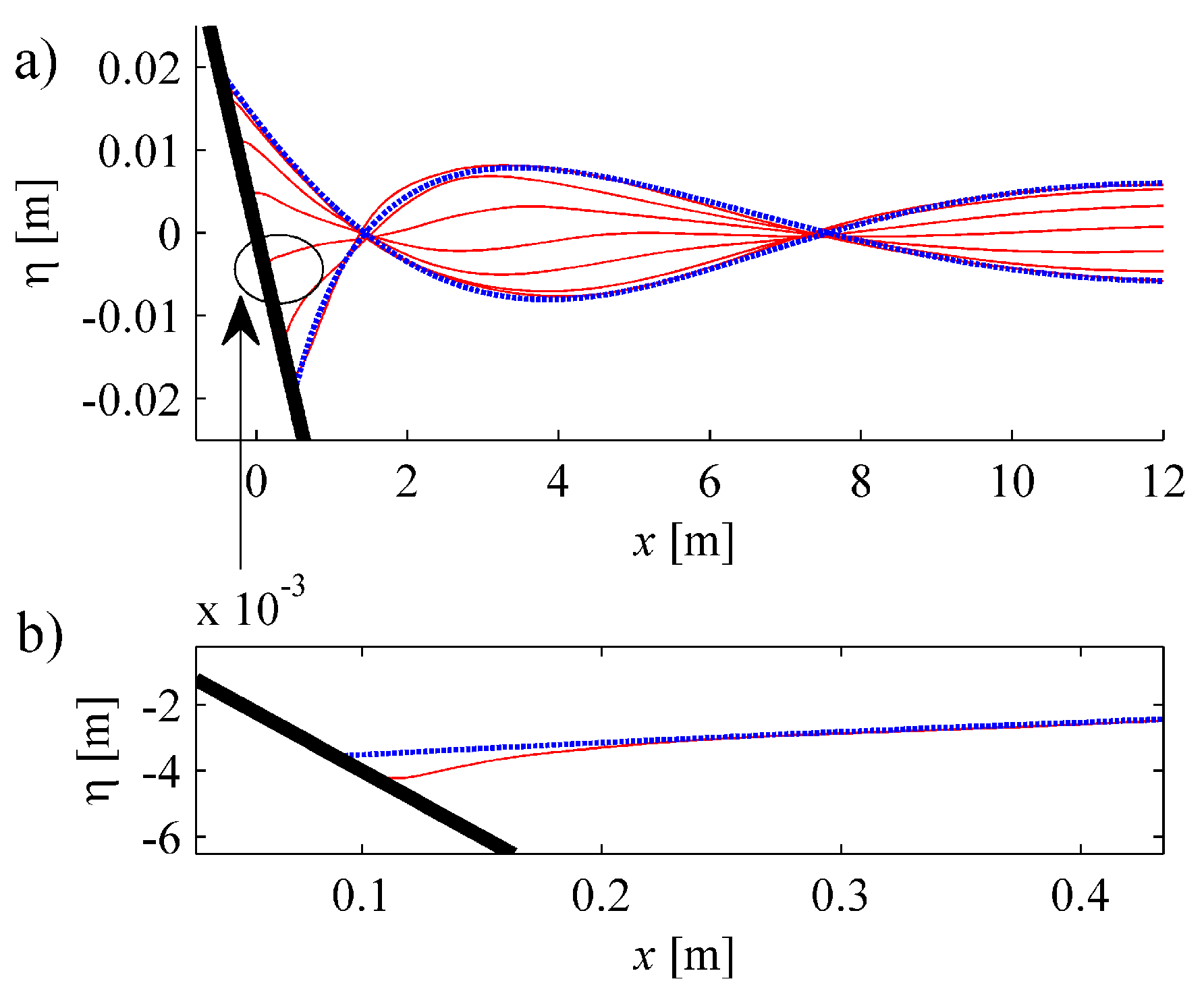
In order to validate the numerical model two comparisons with the results of other authors were performed. A test to propagates a sinusoidal wave train incident an inclined plane was performed. Ref Carrier and Greenspan [28] proposed an analytical solution derived by the Airy’s approximation of the NLSWE. This analytical solution became a standard test for run-up and run-down modelling. A sinusoidal wave, 0.006 m height and a period of 10 s, was used to force the weakly dispersive Boussinesq model. The wave train propagates in a numerical flume with a water depth of 0.5 m and a slope of 1:25. The envelope of the free surface, computed by the weakly dispersive Boussinesq model at different time steps, was plotted in Figure 4 superimposed with the analytical solution of [28]. Figure 4b shows a magnification of an intermediate time step identified with a black circle in Figure 4a.
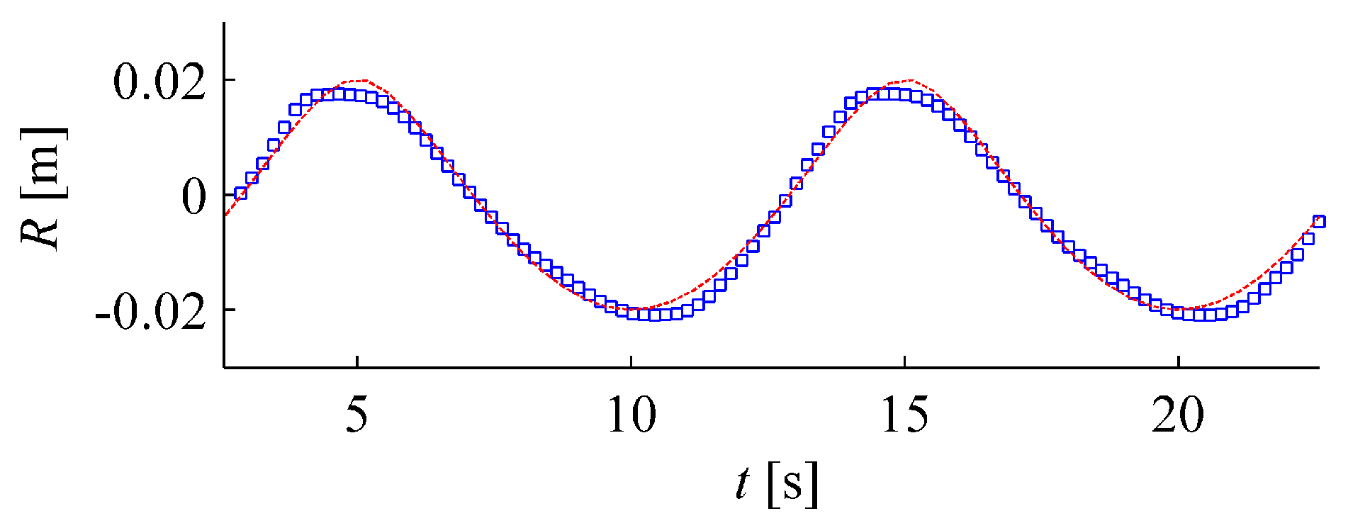
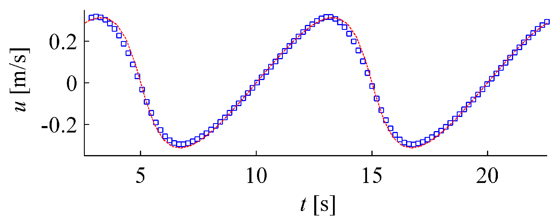
Figure 5 shows the oscillations of the run-up (R), compared to the analytical solution of Carrier and Greenspan [28], nevertheless, the slight underestimation of the maxima of R the result of the non-hydrostatic weakly dispersive model are very good. The proposed model shoreline horizontal velocity was also compared with the analytical solution Figure 6. The horizontal shoreline velocity is almost the same both in the numerical and in the analytical solution.

3.2. The Fringing Reef Experiment

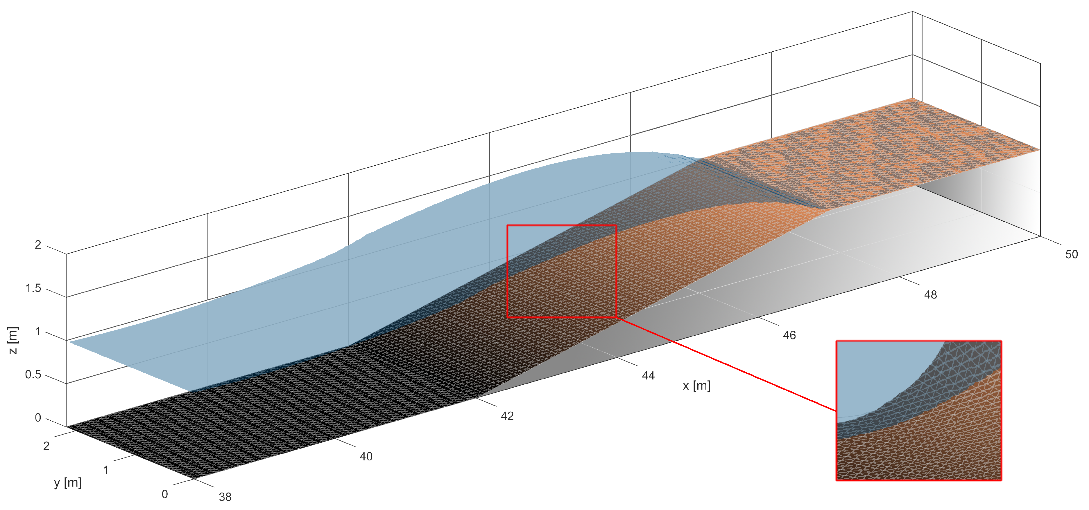
The second test case was the solitary wave propagation over a reef. The wave transformation over an idealized fringing reef highlights the model’s capability in resolving nonlinear dispersive solitary waves, considering also wave breaking. The experiments results used for the comparison were carried out at the O.H. Hinsdale Wave Research Laboratory of Oregon State University where a model of a flat dry reef was used to represent a real fringing reef [5,6]. The numerical model replicated the real flume that was 48.8 m long, 2.16 m wide, and 2.1 m high. The computational grid was simply built with equilateral triangles of edge length equal to 0.08 m. The total number of triangles was 55,550 and the nodes were equal to 28,813 and the time step was d t = 0.02 s. Figure 7 shows the numerical domain and the surface elevation at t * = t · g / h 0 = 55.1 and the red line shows a local zoom of the triangular mesh.
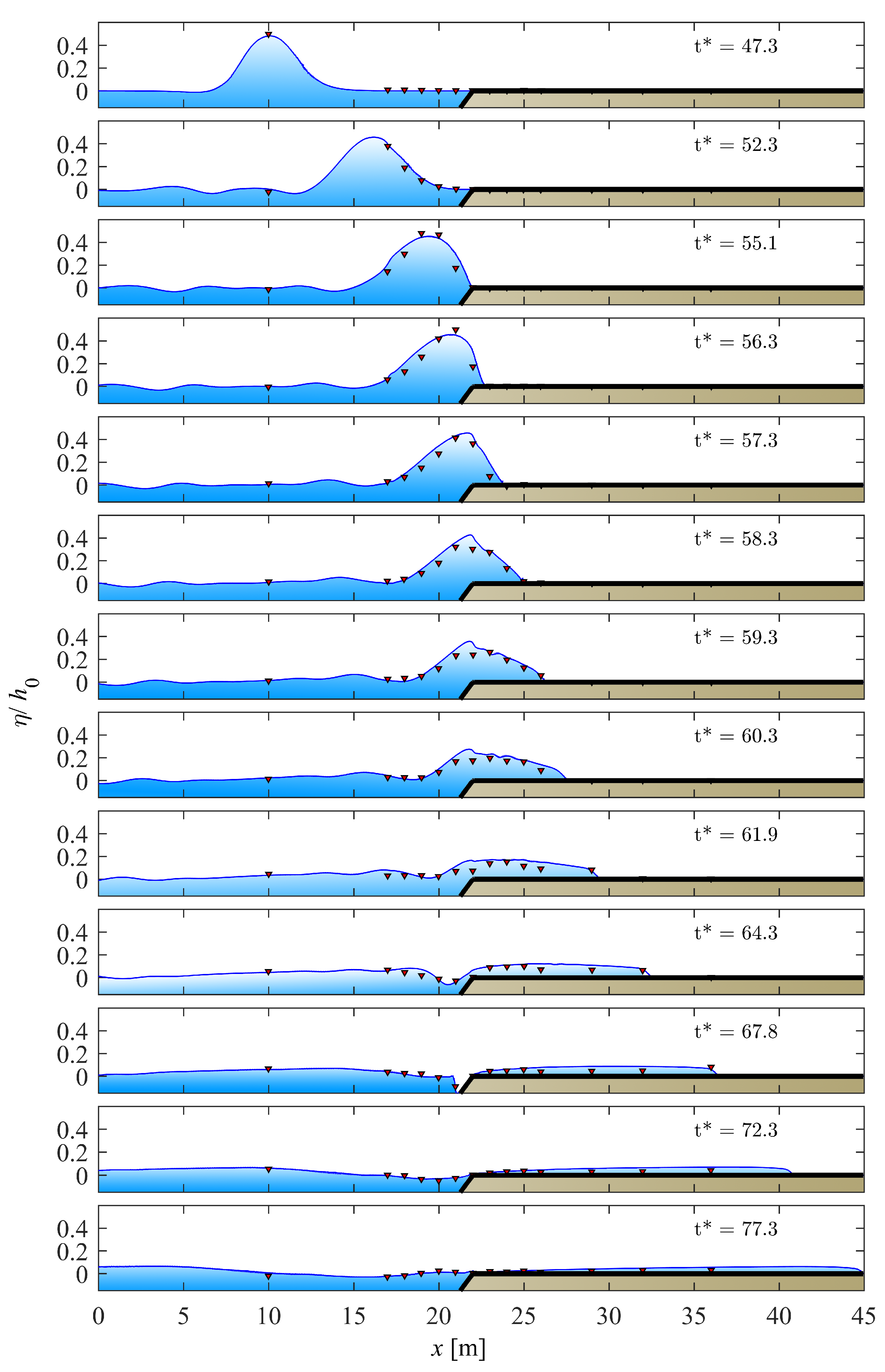
A solitary wave with a dimensionaless wave height of H / h 0 = 0.5 was generated at the inlet of numerical flume and a Manning coefficient n = 0.012 was adopted to reproduce the roughness of the bottom of the flume. In Figure 8 are shown the model results compared to the measured data [5] at 13 dimensionaless time steps t * = t · g / h 0 .
The solitary wave becomes steeper as it propagates over the slope and it rises over the coral reef shoals without breaking into a typical plunge.
In the dimensionless time step t * = 64.3, the numerical model shows a draw-down in front of the flat reef, that produces a back-reflected wave (Figure 8). Instead, the high-speed water sheet over the reef quickly runs up. The numerical model accurately replicated the physics of the phenomenon at each time step (Figure 8). Moreover, the numerical model well reproduces the solitary wave propagation over the edge reef as shown in Figure 9. The time series refers to a point far 22 m from the wavemaker as described in [29], once more the agreement with the numerical model is good.

4. Results and Discussions of a Real Case of Tsunami Propagation

In order to make an inundation map of a small interest area a numerical model was used in the case study of Marzamemi (see Section 2).
A triangular mesh was built using the code proposed by Engwirda [30]. The unstructured mesh has the following characteristics: 11,714 triangles, 5990 nodes (see Figure 10a). The triangles size was determined by means of a density function related to bathymetry, making larger triangles in deeper waters.
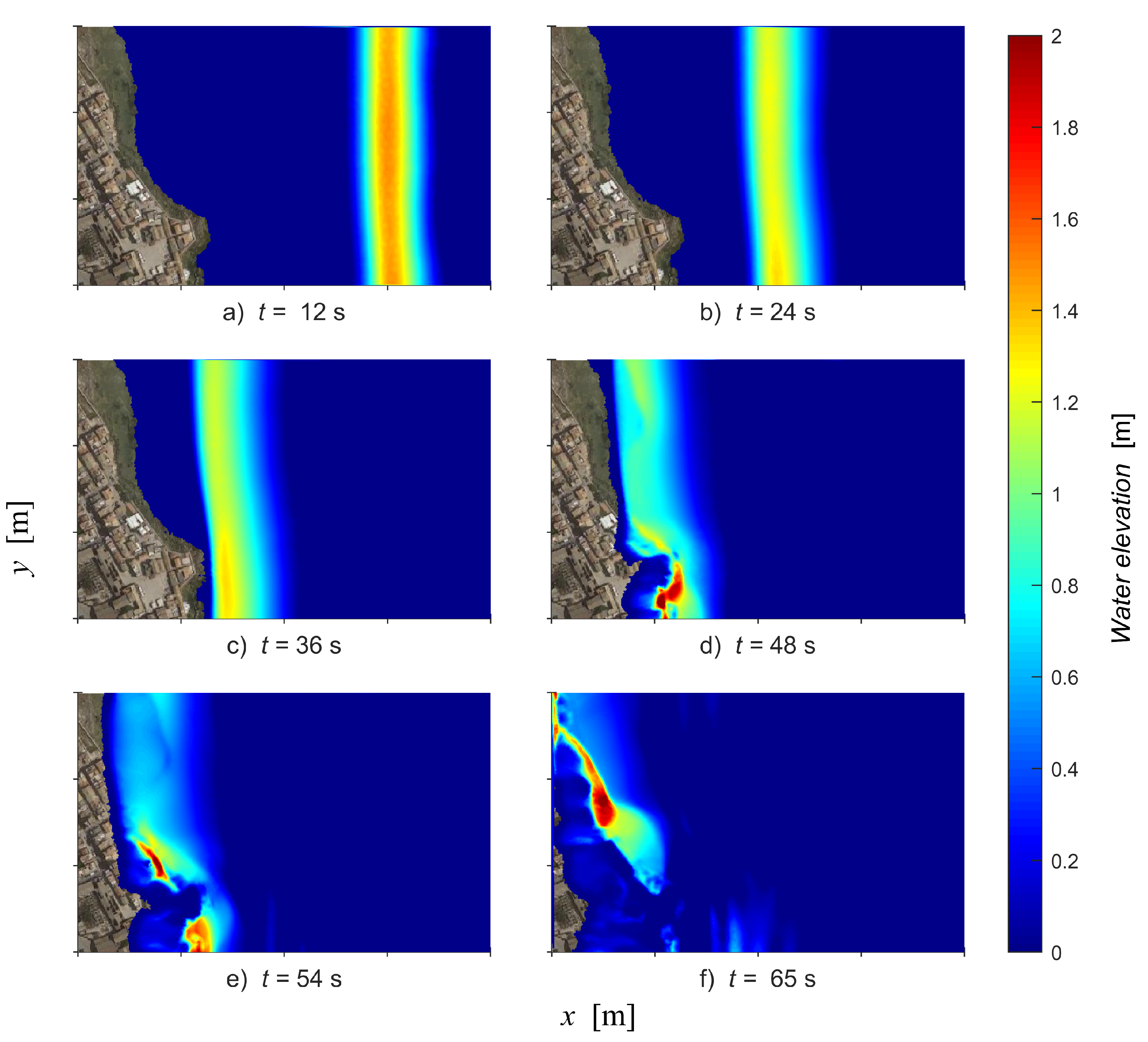
The bathymetry of the model was obtained from regional digital bathymetric charts whereas digital elevation model was built by the regional topographic maps at 1:10,000 scale (see Figure 10b). The two lateral sides of the domain were walls with a free slip condition, in the bottom was calculated a friction term using the Manning’s roughness coefficient equal to 0.012 s/m 1 / 3 see Equations (2) and (3). The adopted time step was Δ t = 0.2 s and the incoming tsunami wave was simulated as 2 m height solitary wave. The propagation of a tsunami wave and the subsequent flooding areas are shown in Figure 11 in which each subplot shows the surface elevation (above Mean Water Level (MWL)) in a specific time after the start of the simulation. At the initial time step a solitary wave, 2 m height, was generated in the eastern domain side, about 500 m far from the coastline. This wave is linked to a possible earthquake with a return period of about 2000 years [31], neglecting a statistical study regarding catastrophic events. The earthquake-induced tsunami is related to a hypocentral point near to seafloor and the fault mechanism is reverse. In particular, it was taken into account, as a potential tsunami source, an earthquake about 200 km far from the coast. It is important to point out that in this manuscript we are presenting a preliminary study. Analysis of tsunami propagation in the Ionian sea area including statistical studies about earthquake-induced tsunami hazard are ongoing.
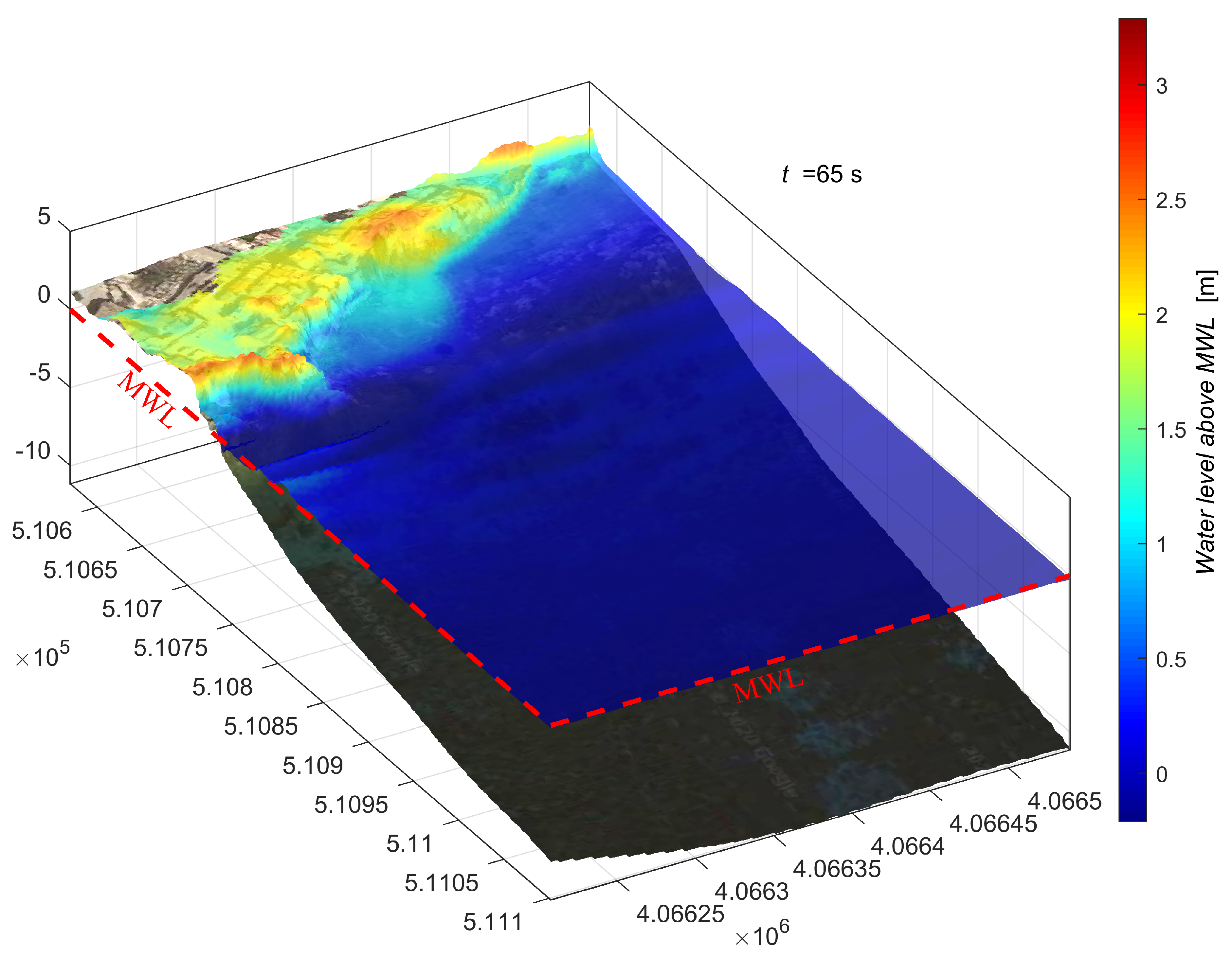
Figure 11 reports the water surface elevation at several time steps. The water elevation was calculated regarding the initial condition (still water level), thus it coincides with the water depth where the points originally were dry. In the subplot (a) of Figure 11, the tsunami propagation at time t = 12 s is shown. In this time the wave is about 300 m far from the coastline and its shape begins to change due to the frequency dispersion. Simultaneously, the wavefront starts to rotate as a result of the change of bathymetry, at the t = 24 s, in Figure 11b, it is clearly distinguishable the refraction process. At t = 36 s Figure 11c, the wave reaches the coast near the most exposed stretch in which there is the main square of the village of Marzamemi. In Figure 11d, t = 48 s, it is described the shoaling of the tsunami and the initial flooding inside the main streets of the village reaching the wave an elevation of 2 m. In this time the northern part of the village is not yet flooded. In the next subplot, (e) t = 54 s, a complete inundation of the main square and the littoral promenade is shown although with small water depth (20–40 cm). At same time step, it is possible to see the wave breaking over the seawall that should protect the habitations and the road infrastructure. The last time step, (f) shows the flooding of the whole studied coastal area. A magnification of the last time step of the simulation is shown in Figure 12 with the x and y coordinates in the local reference system and the water height measured above the MWL. At t = 65 s, the church and the ancient tuna factory, XV century, were flooded.

5. Concluding Remarks

In this paper, preliminary studies regarding the tsunami flooding hazards were presented. The tsunami is an highly nonlinear and dispersive wave and it must be modeled using appropriated numerical model. Indeed, the adopted Boussinesq type of model, in its category of depth integrated, guarantees a balance between the frequency dispersion and non-linearity. Moreover, it was possible, by means of the Delaunay mesh grid, to have very detailed results with a minor computational cost. As a consequence of this, the model better assess the coastal flooding hazard. The numerical model was validated through the analytical solution of Carrier and Greenspan [28] and with the experimental study presented by Roeber et al. [5]. The comparisons with the numerical model show excellent agreements. Finally, it was applied the numerical modeling procedure to a real case in order to perform the propagation of the tsunami and to evaluate its impact on the coast and the subsequent coastal flooding. To assess both the possibility of coastal flooding and their extent, an earthquake, that cause a tsunami, was generated off the Ionian coast (return period c.a. 2000 years).The results of the tsunami propagation show that the extent of the flooded areas is about 100 m inward the shoreline. All roads near the shoreline, including the historic village square, are flooded. The water levels, although not extremely high, could cause dangers mainly in the periods of the year when the population density grows considerably. These results, although preliminary, highlight the extreme fragility of this coastal site. For this reason, further numerical modeling is ongoing, taking into account also the structural response of the buildings inside the village of Marzamemi. This preliminary investigation is the basis for further studies that are already underway, their results will be useful for civil protection agencies in order to project emergency management plans.

Author Contributions

Data curation, C.L.R. and G.M.; Formal analysis, C.L.R. and G.M.; Methodology, C.L.R., G.M., and G.C.; Software, C.L.R. and G.M.; Supervision, G.C.; Geological and geomorphological supervision, G.M.; Hydarulic modelling C.L.R.; Writing—original draft, C.L.R., G.M. and G.C.; Writing—review & editing, C.L.R., G.M. and G.C. All authors have read and agreed to the published version of the manuscript.

Funding

This research was funded by SIMIT THARSY Tsunami Hazard Reduction System C1-3.2-5-INTERREG V-A Italia-Malta.The APC was funded by SIMIT THARSY.

Acknowledgments

We thank our scientific responsible, Goffredo La Loggia, for assistance to tasks development during the project SIMIT-THARSY.

Conflicts of Interest

The authors declare no conflict of interest.

References

  1. Molina, R.; Manno, G.; Lo Re, C.; Anfuso, G.; Ciraolo, G. Storm Energy Flux Characterization along the Mediterranean Coast of Andalusia (Spain). Water 2019, 11, 509. [Google Scholar] [CrossRef] [Green Version]
  2. Molina, R.; Manno, G.; Lo Re, C.; Anfuso, G.; Ciraolo, G. A Methodological Approach to Determine Sound Response Modalities to Coastal Erosion Processes in Mediterranean Andalusia (Spain). J. Mar. Sci. Eng. 2020, 8, 154. [Google Scholar] [CrossRef] [Green Version]
  3. Manno, G.; Lo Re, C.; Ciraolo, G. Uncertainties in shoreline position analysis: The role of run-up and tide in a gentle slope beach. Ocean Sci. 2017, 13, 661–671. [Google Scholar] [CrossRef] [Green Version]
  4. Lo Re, C.; Musumeci, R.E.; Foti, E. A shoreline boundary condition for a highly nonlinear Boussinesq model for breaking waves. Coast. Eng. 2012, 60, 41–52. [Google Scholar] [CrossRef]
  5. Roeber, V.; Cheung, K.F.; Kobayashi, M.H. Shock-capturing Boussinesq-type model for nearshore wave processes. Coast. Eng. 2010, 57, 407–423. [Google Scholar] [CrossRef]
  6. Roeber, V.; Cheung, K.F. Boussinesq-type model for energetic breaking waves in fringing reef environments. Coast. Eng. 2012, 70, 1–20. [Google Scholar] [CrossRef]
  7. Zhang, H.; Zhang, M.; Ji, Y.; Wang, Y.; Xu, T. Numerical study of tsunami wave run-up and land inundation on coastal vegetated beaches. Comput. Geosci. 2019, 132, 9–22. [Google Scholar] [CrossRef]
  8. Marivela, R.; Weiss, R.; Synolakis, C. The Temporal and Spatial Evolution of Momentum, Kinetic Energy and Force in Tsunami Waves during Breaking and Inundation. arXiv 2016, arXiv:1611.04514. [Google Scholar]
  9. Manoj Kumar, G.; Sriram, V.; Didenkulova, I. A hybrid numerical model based on FNPT-NS for the estimation of long wave run-up. Ocean Eng. 2020, 202, 107181. [Google Scholar] [CrossRef]
  10. Wei, Z.; Dalrymple, R.A.; Rustico, E.; Hérault, A.; Bilotta, G. Simulation of Nearshore Tsunami Breaking by Smoothed Particle Hydrodynamics Method. J. Waterway Port Coast. Ocean Eng. 2016, 142, 05016001. [Google Scholar] [CrossRef]
  11. Qin, X.; Motley, M.; LeVeque, R.; Gonzalez, F.; Mueller, K. A comparison of a two-dimensional depth-averaged flow model and a three-dimensional RANS model for predicting tsunami inundation and fluid forces. Nat. Hazards Earth Syst. Sci. 2018, 18, 2489–2506. [Google Scholar] [CrossRef] [Green Version]
  12. Qu, K.; Ren, X.; Kraatz, S. Numerical investigation of tsunami-like wave hydrodynamic characteristics and its comparison with solitary wave. Appl. Ocean Res. 2017, 63, 36–48. [Google Scholar] [CrossRef]
  13. Arico, C.; Lo Re, C. A non-hydrostatic pressure distribution solver for the nonlinear shallow water equations over irregular topography. Adv. Water Resour. 2016, 98, 47–69. [Google Scholar] [CrossRef] [Green Version]
  14. Presti, V.L.; Antonioli, F.; Auriemma, R.; Ronchitelli, A.; Scicchitano, G.; Spampinato, C.; Anzidei, M.; Agizza, S.; Benini, A.; Ferranti, L.; et al. Millstone coastal quarries of the Mediterranean: A new class of sea level indicator. Quat. Int. 2014, 332, 126–142. [Google Scholar] [CrossRef]
  15. Samaras, A.; Karambas, T.V.; Archetti, R. Simulation of tsunami generation, propagation and coastal inundation in the Eastern Mediterranean. Ocean Sci. 2015, 11, 643–655. [Google Scholar] [CrossRef] [Green Version]
  16. Schambach, L.; Grilli, S.T.; Kirby, J.T.; Shi, F. Landslide Tsunami Hazard Along the Upper US East Coast: Effects of Slide Deformation, Bottom Friction, and Frequency Dispersion. Pure Appl. Geophys. 2019, 176, 3059–3098. [Google Scholar] [CrossRef]
  17. Mueller, C.; Micallef, A.; Spatola, D.; Wang, X. The Tsunami Inundation Hazard of the Maltese Islands (Central Mediterranean Sea): A Submarine Landslide and Earthquake Tsunami Scenario Study. Pure Appl. Geophys. 2020, 177, 1617–1638. [Google Scholar] [CrossRef]
  18. Suardana, A.M.A.P.; Sugianto, D.N.; Helmi, M. Study of Characteristics and the Coverage of Tsunami Wave Using 2D Numerical Modeling in the South Coast of Bali, Indonesia. Int. J. Oceans Oceanogr. 2019, 13, 237–250. [Google Scholar]
  19. Papadopoulos, G.A.; Fokaefs, A. Strong tsunamis in the Mediterranean Sea: A re-evaluation. ISET J. Earthq. Technol. 2005, 42, 159–170. [Google Scholar]
  20. DISS Working Group. Database of Individual Seismogenic Sources (DISS). In A Compilation of Potential Sources for Earthquakes Larger than M 5.5 in Italy and Surrounding Areas; Istituto Nazionale di Geofisica e Vulcanologia: Rome, Italy, 2018. [Google Scholar] [CrossRef]
  21. Caputo, R.; Pavlides, S. The Greek Database of Seismogenic Sources (GreDaSS), version 2.0.0: A Compilation of Potential Seismogenic Sources (Mw > 5.5) in the Aegean Region; University of Ferrara: Ferrara, Italy, 2013. [Google Scholar] [CrossRef]
  22. Gutscher, M.A.; Roger, J.; Baptista, M.A.; Miranda, J.M.; Tinti, S. Source of the 1693 Catania earthquake and tsunami (southern Italy): New evidence from tsunami modeling of a locked subduction fault plane. Geophys. Res. Lett. 2006, 33, L08309. [Google Scholar] [CrossRef] [Green Version]
  23. Catalano, R.; Doglioni, C.; Merlini, S. On the mesozoic Ionian basin. Geophys. J. Int. 2001, 144, 49–64. [Google Scholar] [CrossRef] [Green Version]
  24. Papadopoulos, G.A.; Daskalaki, E.; Fokaefs, A.; Giraleas, N. Tsunami hazard in the Eastern Mediterranean sea: Strong earthquakes and tsunamis in the west Hellenic arc and trench system. J. Earthq. Tsunami 2010, 4, 145–179. [Google Scholar] [CrossRef]
  25. LeVeque, R.J. Numerical Methods for Conservation Laws; Birkhäuser Boston: Basel, Switzerland, 2013. [Google Scholar]
  26. Toro, E.F. Riemann Solvers and Numerical Methods for Fluid Dynamics: A Practical Introduction; Springer Science & Business Media: New York, NY, USA, 2013. [Google Scholar]
  27. Stelling, G.S.; Duinmeijer, S.P.A. A staggered conservative scheme for every Froude number in rapidly varied shallow water flows. Int. J. Numer. Methods Fluids 2003, 43, 1329–1354. [Google Scholar] [CrossRef]
  28. Carrier, G.; Greenspan, H. Water waves of finite amplitude on a sloping beach. J. Fluid Mech. 1958, 4, 97–109. [Google Scholar] [CrossRef]
  29. Roeber, V. Boussinesq-Type Model for Nearshore Wave Processes in Fringing Reef Environment. Ph.D. Thesis, University of Hawaii at Manoa, Honolulu, HI, USA, December 2010. [Google Scholar]
  30. Engwirda, D. Locally-Optimal Delaunay-Refinement and Optimisation-Based Mesh Generation. Ph.D. Thesis, The University of Sydney, Sydney, Australia, 2014. [Google Scholar]
  31. Basili, R.; Brizuela, B.; Herrero, A.; Iqbal, S.; Lorito, S.; Maesano, F.E.; Murphy, S.; Perfetti, P.; Romano, F.; Scala, A.; et al. NEAM Tsunami Hazard Model 2018 (NEAMTHM18): Online Data of the Probabilistic Tsunami Hazard Model for the NEAM Region from the TSUMAPS-NEAM Project; Istituto Nazionale di Geofisica e Vulcanologia (INGV): Roma, Italy, 2018. [Google Scholar] [CrossRef]
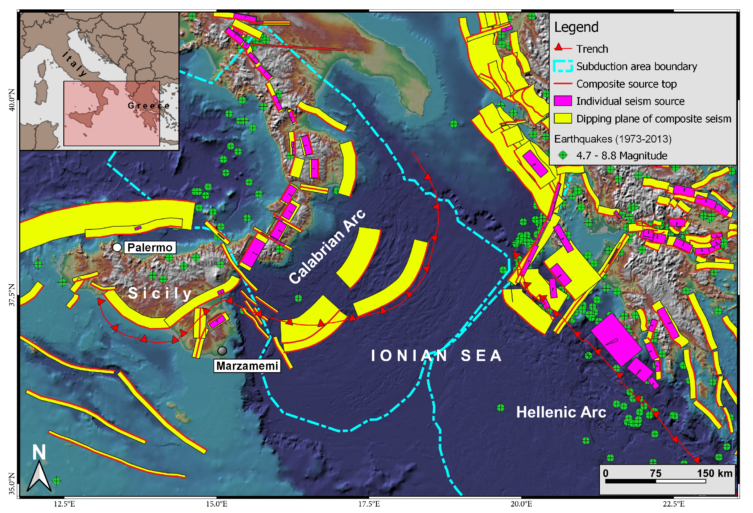
Figure 1. Possible seismic sources in the Ionian Sea. The data-set is taken from the DISS Working Group [20], Caputo and Pavlides [21].
Water 12 01448 g001
Figure 2. The case study area. The red rectangle shows the Marzamemi promontory, the yellow dash-dot line highlights the boundaries of the numerical model.
Water 12 01448 g002
Figure 3. Definition scheme of the adopted variables.
Water 12 01448 g003
Figure 4. (a) Envelope of free surface of sine wave run-up on a planar beach. Comparison between the weakly dispersive model (blue dotted lines) and Carrier and Greenspan [28] analytical solution (continuous red lines). (b) A zoom of the surface elevation near the planar beach at an intermediate time step.
Water 12 01448 g004
Figure 5. Shoreline vertical motion R of sine wave run-up on a planar beach. Comparison between adopted model (blue dotted lines) and the analytical solution by Carrier and Greenspan [28] (continuous red lines).
Water 12 01448 g005
Figure 6. Shoreline velocity of monochromatic wave run-up on a planar beach. Comparison between adopted model (blue dotted lines) and the analytical solution by Carrier and Greenspan [28] (continuous red lines).
Water 12 01448 g006
Figure 7. The numerical domain and the triangular equilateral mesh used in the flat reef run-up test. The red box highit a magnified area of the mesh. The surface elevation correspond to t * = 55.1 .
Water 12 01448 g007
Figure 8. Surface elevations of solitary wave over a flat reef with H / h 0 = 0.5 and 1:5 slope. Solid blue lines are the weakly dispersive model results and the red triangles are measured data. Each subplot shows the results at a dimensionaless time step.
Water 12 01448 g008
Figure 9. Time series of the surface elevation at edge of the reef. The blue line is the numerical model results the red circles are the measurements by [29].
Water 12 01448 g009
Figure 10. The Marzamemi numerical domain. (a) The used triangular mesh, (b) the bathymethry of the studied area, the color bar shows the elevation in meters above mean water level. In the subplots the coordinate origin are E = 510,569 m; N = 4,066,207 m; WGS84-UTM33N reference system.
Water 12 01448 g010
Figure 11. Water surface elevation. The origin of coordinate axis is E = 510,569 m; N = 4,066,207 m; WGS84 UTM33N reference system.
Water 12 01448 g011
Figure 12. Magnification of subplot (f) of Figure 11. The red lines shows the MWL the color bar shows the water level above the MWL.
Water 12 01448 g012