Article

Evaluation of Uncertainty Intervals for Daily, Statistically Derived Streamflow Estimates at Ungaged Basins across the Continental U.S.

1
U.S. Geological Survey, Mounds View, MN 55112, USA
2
U.S. Geological Survey, Lakewood, CO 80225, USA
*
Author to whom correspondence should be addressed.
Water 2020, 12(5), 1390; https://doi.org/10.3390/w12051390
Submission received: 3 April 2020 / Revised: 4 May 2020 / Accepted: 5 May 2020 / Published: 14 May 2020

Abstract

:
Streamflow estimation methods that transfer information from an index gage to an ungauged site are commonly used; however, uncertainty in daily streamflow estimates are often not adequately quantified. In this study, daily streamflow was simulated at 1331 validation streamgauges across the continental United States using four transfer-based streamflow estimation methods. Empirical 95 percent uncertainty intervals were computed for estimated daily streamflows. Uncertainty intervals were evaluated for reliability, sharpness, and overall ability to accurately quantify the uncertainty inherent in the estimated daily streamflow. Uncertainty intervals performed reliably in the Eastern U.S. and Pacific Northwest regions of the country, containing a median of 96 and 99 percent of the observed values respectively. Uncertainty intervals were less reliable in the Great Plains and arid Southwest regions, where uncertainty intervals contained a median of 83 and 94 percent of the observed streamflows respectively. Uncertainty interval performance was correlated with gage density and hydrologic similarity near the validation site, as well as the aridity and baseflow indices at the site.

1. Introduction

Daily streamflow data are required in many water resources applications to characterize the quantity, timing, and frequency of high and low streamflow events at a location of interest. Applications requiring such information are wide ranging and include water availability assessments, dam operations, ecological protection and restoration, and urban land use planning and development [1,2,3,4]. While streamgage measurements are the best source of daily streamflow data, it is not feasible to operate long term continuous streamgages at every location of interest nor at every location that might be of interest in the future. When daily streamflow is needed but a streamgage is not available, streamflow may be estimated using process-based numerical models or statistical, transfer-based methods.
Process- and transfer-based models estimate ungaged streamflow in inherently different ways. Process models attempt to numerically represent the physical linkages of hydrologic processes such as evaporation, precipitation, or infiltration. In contrast, transfer-based models use various numerical transformations or statistical methods to infer the timing and magnitude of daily streamflow at an ungaged site from those at gaged sites. Transfer-based methods are sometimes preferred because of the time and data demands involved in developing and calibrating a process-based numerical model [5]. Both process-based and transfer-based models provide deterministic estimates of streamflow with little characterization of model uncertainty. This study evaluates a method to assess uncertainty in deterministic models and documents the sensitivity of these methods to heterogeneous hydrologic conditions for two common transfer-based streamflow estimation methods.
The drainage area ratio method (DAR) is a straightforward transfer-based method of streamflow estimation in which streamflow at an index gage is scaled by the ratio of the drainage areas of the gaged and unaged site [6]. The DAR method has been shown to be accurate and unbiased in a number of regional studies [7,8,9,10]. Previous attempts to refine DAR methods include the use of an exponential scaling factor [9] or the incorporation of information from multiple index gages [5]. The DAR method is widely used because of its ease of application. However, few applications have considered the uncertainty of streamflow values estimated by the DAR method.
Nonlinear spatial interpolation using flow duration curves (QPPQ) use regional regression equations and interpolation to estimate a continuous flow duration curve at an ungaged site and then distributes the flow durations into a daily time series using streamflow from an index gage [11,12,13,14]. One advantage to this method is its ability to incorporate physiographic information from a basin in addition to the drainage area in order to explain variability in regional streamflow patterns. This method has been applied in many regions of the U.S. [14,15,16,17] under various names and is referred to in this document as the QPPQ method, as first described by Fennesey [11]. While it is possible to quantify the uncertainty in the flow duration curve quantiles when standard methods (e.g., regression-based regionalization) are used, it is unclear how that uncertainty can be translated into the resulting time series of estimated streamflow.
Both the DAR and QPPQ methods are popular and can provide reasonable estimates of streamflow at an ungaged location, but the uncertainty associated with daily streamflow estimates is often not adequately characterized or considered in the applications in which they are used. When described, the accuracy of these methods is typically presented as the Nash–Sutcliffe Efficiency (NSE) [18], average percent error, or other metrics of overall goodness of fit [19]. While these are important measures of overall model accuracy, they do not provide any information about the uncertainty of individual daily streamflow estimates. Understanding the uncertainty of specific estimates may be essential to inform water resource management.
One reason uncertain information is often omitted in streamflow estimation studies is that both process-based and transfer-based methods are less parametric than traditional statistical methods which complicates efforts to characterize uncertainty in any formal way. Consider a tool like ordinary least squares regressions: one can make parametric and nonparametric assumptions that allow for a characterization of parameter and prediction uncertainty. Of course, violating these assumptions limits the utility of uncertainty estimators. The practice of hydrograph simulation is an applied science that lacks such a theoretical underpinning. In the case of process-based methods, which attempt to represent underlying physical processes through mathematics, the study of uncertainty propagation is nascent. With transfer-based methods, it is perhaps possible to characterize some uncertainty (e.g., in regionalized flow duration curves of the QPPQ method), but how uncertainty is transferred across index gages is less well understood.
Bourgin et al. [20] introduced a method of estimating empirical uncertainty intervals for daily streamflow estimates from a rainfall runoff model at an ungaged location. The method uses distributions of error ratios from streamflow simulations at hydrologically similar gaged sites to estimate the uncertainty at an ungaged location. While Bourgin et al. applied the method to outputs from process-based models, the methodology could be similarly applied to transfer-based methods. Farmer and Levin [21] modified the method for use with a QPPQ simulation of daily streamflow in Massachusetts and showed that the method was generally reliable for characterizing the uncertainty in daily streamflow in this application. The performance of this method relies upon the ability to find a sufficient number of index gages that are hydrologically similar to the ungaged location. Streamflows in Massachusetts exhibit a high degree of hydrologic similarity and benefit from a dense network of daily streamflow gages, making it an ideal location for the implementation of these types of transfer-based simulation methods and uncertainty characterization. The method has not been applied in more hydrologically diverse regions such as semi-arid and arid environments which may exhibit less hydrologic similarity between streams. This study applies the empirical uncertainty intervals across the continental United States and assesses the capability of the uncertainty intervals to accurately characterize uncertainty in estimated daily streamflow across a wide range of hydrologic regimes.

2. Materials and Methods

2.1. Study Area

Daily streamflow was estimated through a leave-one-out cross-validation procedure at 1331 gaged locations across the conterminous U.S from the period of 1 October 1980 through 30 September 2013 (Figure 1) to simulate the application of these methods at ungaged locations. The Gages-II data set [22] designates streamgages in basins that are minimally altered by human modification, dams, or water use, as reference gages. All locations were designated as a reference gage in the Gages-II dataset [22], had a period of record of at least 10 complete water years, and had non-zero streamflow for at least 50% of the period of record. The drainage areas of the selected sites ranged from 1.5 to 25,791 km2. Gages used in this study, as well as observed data, metadata, and source code for all streamflow and confidence interval estimations are available in Levin [23].
Gage density—the number of streamgages per unit area—varies considerably across the U.S. Gage density is greatest in the Pacific Northwest mountain region and the Eastern U.S., with median gage densities of 82 and 105 gages per 500,000 km2, respectively. Gages in these regions had a median distance of 17.3 km and 23.4 km, respectively, between them and the next nearest gage. Gage density was lowest in the Great Plains and arid Southwest regions with a median gage density of 46 and 48 gages per 500,000 km2, respectively, and a median minimum distance of 29.0 and 30.8 km between gages, respectively. The Gages-II data set includes basin characteristics for each site compiled from various national scale data sets and include various climate, hydrologic, geologic, land use, and topographic categories [22]. These variables were used to examine potential correlations between basin characteristics and uncertainty interval performance.

2.2. Streamflow Estimation Methods

Daily streamflow was estimated at each of the 1331 validation sites using two statistical, transfer-based methods which require the use of an index gage to determine the timing and magnitude of daily streamflow: the drainage area ratio method (DAR) and nonlinear spatial interpolation using flow duration curves (QPPQ). As the applications presented here are based on previous work [11,14,20,21], the description of methods provided here covers only the necessary fundamentals to understand the methods. Readers interested in the detailed development of each method are referred to the literature cited.
The drainage area ratio is simple to implement, requiring only a time series of index gage streamflows and the drainage areas of both the ungaged and index sites. The DAR method assumes the streamflow per unit area is equivalent at the ungaged and index-gaged basins and computes the daily streamflow at the ungaged basin as:
Q ^ u = Q i ( A u A i )
where Q ^ u and Q i are the daily streamflow at the ungaged and index gage site, respectfully and Au and Ai are the drainage areas of the ungaged and index gaged basins, respectfully.
The application of the QPPQ method explored here uses regionalized regression equations to estimate streamflow quantiles at an ungaged site and an index gage to transform the flow duration curve into a daily time series. The regression-estimated streamflow quantiles are interpolated to produce a continuous flow duration curve. Then, the flow duration curve is parsed into a daily time series by assuming that the exceedance probability streamflow at the ungaged location occurs on the same day as the corresponding exceedance probability streamflow at an index gage. For example, if the streamflow at the index site on the first of January 2009 has an exceedance probability of 67%, then this same exceedance probability will be assumed for the first of January 2009 at the ungaged location. Absolute magnitude is then obtained by interpolating the exceedance probability of streamflow (67%, in this case) along the estimated flow duration curve at the target location.
To apply the QPPQ method at each validation site, an automated process was used to develop regression equations for streamflow at 27 quantiles with exceedance probabilities of 0.02, 0.05, 0.1, 0.2, 0.5, 1, 2, 5, 10, 20, 25, 30, 40, 50, 60, 70, 75, 80, 90, 95, 98, 99, 99.5, 99.8, 99.9, 99.95, and 99.98 percent. Streamflow data and basin characteristics from the Gages-II data set from all reference gages within a 400 km radius of the target site were used to fit the regression equations. Regression equations for the 27 exceedance probabilities were fitted at each validation site using an automated regression fitting and selection process as described by [24]. This method considers a wide range of covariates for each streamflow quantile, building candidate regression based on an exhaustive “best-subsets” procedure. Final regression equations all included the drainage area as an independent variable. Additionally, final regression equations were constrained such that the maximum number of independent variables was the minimum of N/20 (where N is the number of index gages) or 6 [22,24]. The best-subsets procedure builds all candidate models of a specified size (one, two, or three, etc., covariates) and ranks them by performance (here, defined by adjusted-R-squared). As the models are built independently for each quantile, a post-processing procedure is applied to limit the variability of included covariates by quantile. As described by Over et al. [24], consecutive quantiles are lumped into regimes (e.g., low, medium and high flows), and each quantile within a regime is estimated with the same covariates, determining the set of covariates that produces the best average performance across the regime.

2.3. Index Gage Selection Methods

Each streamflow method requires the use of an index gage to transfer the timing of the streamflows into a daily time series. Typically, the selection of an index gage hinges on some belief about hydrologic similarity for the intended application [25,26]. Two methods of index gage selection were used for each streamflow estimation method: nearest neighbor and map correlation. Nearest neighbor (NN) index selection uses the index gage closest in distance to the ungaged site [26], assuming separation distance to be a proxy for hydrologic similarity. Map correlation (MC) index selection hypothesizes that hydrologic similarity can be represented by the correlation of daily time series and that there is a relation between separation distance and correlation [25]. MC uses ordinary kriging to estimate the correlation of the streamflows at the ungaged site to all other nearby index gaged sites and chooses the index gage site with the highest predicted correlation [25]. In cases where the period of record at an index gage did not fully overlap the simulation period, the next-ranked index gage was chosen to estimate flows for the remaining time period.
The combination of two simulation and two index gage selection methods resulted in 4 unique time series of estimated streamflow at each validation site: NN-DAR, MC-DAR, NN-QPPQ, and MC-QPPQ. For each method, a leave-one-out cross-validation procedure was applied. One gaged site was selected to stand in as the target (ungaged) site. For the purposes of simulation, the streamflow record at this site was set aside. Using the records from the remaining gaged sites, the daily streamflow was simulated at the target site following each of the four methods. The gaged flow at the target site was then reintroduced to assess performance, representing an assessment of a completely ungaged site. Each gaged site was taken, in turn, to be the target site to allow for an analysis of performance across a range of hydroclimatic conditions.

2.4. Uncertainty Characterization

Uncertainty in streamflow simulations was estimated by developing uncertainty intervals for each daily streamflow estimate. Uncertainty intervals were constructed using a process developed by Bourgin et al. [20] for a distributed rainfall-runoff model and modified for use in a regional application of the QPPQ method by Farmer and Levin [21]. The process assumes that the distribution of relative errors of estimated streamflows at an ungaged location is similar to the distribution of relative errors of estimated streamflows at a hydrologically similar, gaged location. If this assumption is true, the relative errors of estimated streamflow at nearby gaged sites can be used to estimate the uncertainty at the ungaged site.
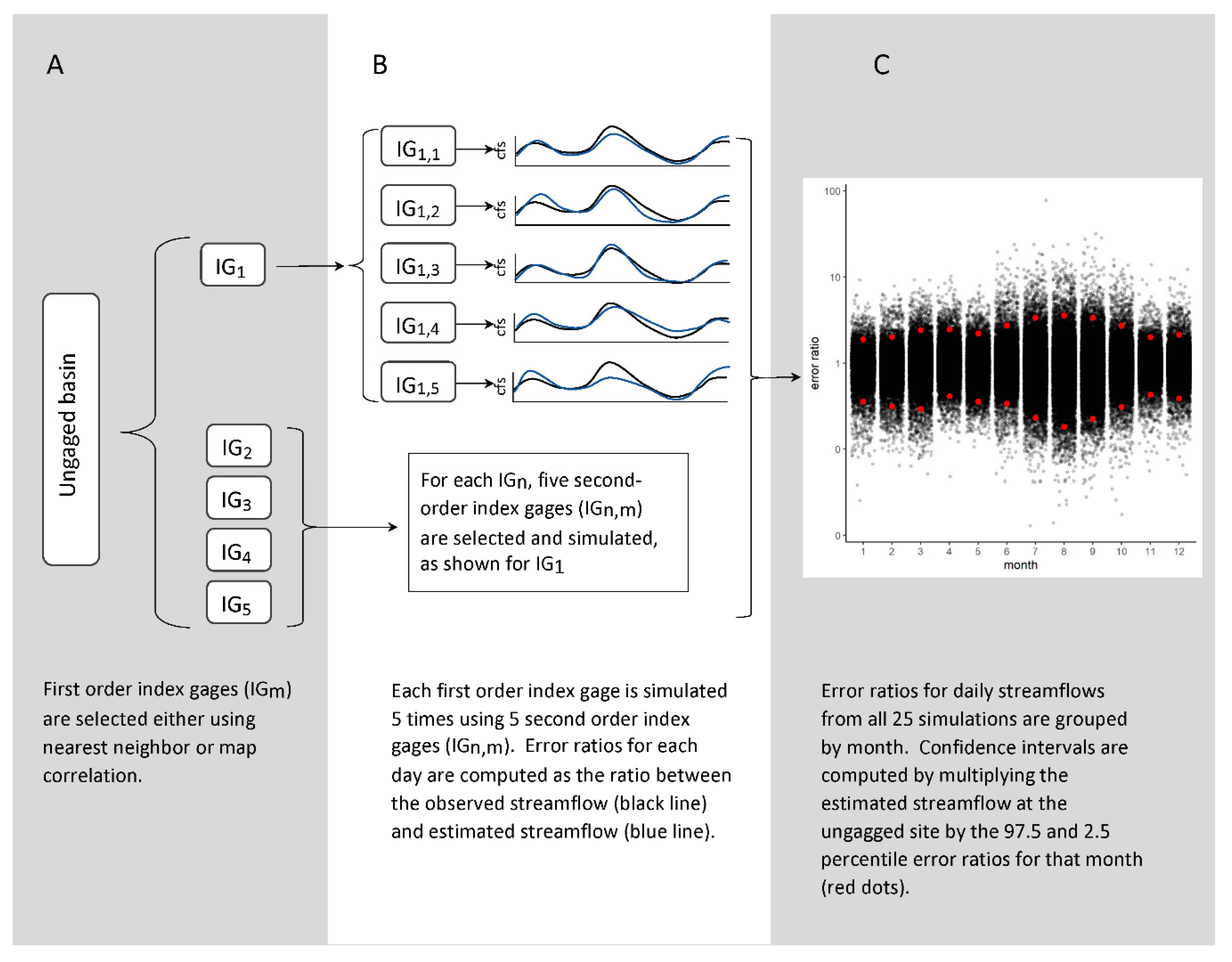
The process to estimate uncertainty intervals for daily streamflow at an ungaged site is summarized in Figure 2 (adapted from Farmer and Levin [21]) and described here. After simulating daily streamflows at the target (ungaged) site, potential index gages are ranked either by distance to the target site (for nearest neighbor simulations) or by the estimated correlation to the target site (for map correlation simulations). The five top-ranked index gages are chosen as first-order index gages (Figure 2A). Each first-order index gage is treated as it if were ungaged and is simulated using the selected simulation method (QPPQ or DAR) five times, using five second-order index gages (Figure 2B). Second order index gages are chosen such that the similarity metric (either distance for NN or predicted correlation for MC) is as close as possible to the similarity metric between the target site and the first-order index gage. For example, if the distance between the target site and the first-order index gage is 10 km, the second order index gages (IGn,m) will be ranked by their distance to the first-order index gage and the five gages with distances nearest to 10 km would be chosen for the simulation. In simulating the daily streamflow at the first-order index gages a leave-two-out procedure was necessary. That is, the gaged streamflow of both the initial target site and the first-order index gage site being considered were set aside for simulation of the first-order index gage. This process results in 5 estimated daily time series for each first-order index gage.
Gaged data at the first-order index gages were used to compute daily error ratios, defined as the ratio of the observed daily streamflow to the simulated daily streamflow, for each of the 25 estimated time series (Figure 2C). In order to facilitate log transformation and prevent error ratios with zero in the denominator, a value of 0.0001 m3/s (0.0049 ft3/s) was added to all daily streamflow data and simulated streamflows were censored at this value. Because the distribution of error ratios may vary according to streamflow magnitude and timing, the streamflows and associated error ratios were grouped by month. In an effort to approximate the 95 percent uncertainty intervals, error ratios with 0.025 and 0.975 non-exceedance probability were computed from the distribution of error ratios for each month. These error ratios were applied multiplicatively to the estimated daily streamflow to produce the upper and lower bounds of the uncertainty interval:
p 2.5 , d × Q ^ u < Q ^ u < p 97.5 , d × Q ^ u
where p2.5,d and p97.5,d are the monthly error ratios with non-exceedance probabilities of 0.025 and 0.975. While Farmer and Levin [21] used monthly error bins, other studies [20,27] binned error ratios by streamflow decile rather than by month. Initial exploration here found that binning by decile had only a marginal effect on the accuracy of uncertainty intervals and often produced erratic interval widths when streamflows in different deciles occur consecutively in the target site daily time series. Monthly binning produced smoother, more continuous uncertainty intervals of daily streamflow, without affecting overall performance. In some cases, target gage simulations used more than one index gage when the primary index gage period of record did not cover the full simulation time period. For these cases, the uncertainty interval process was completed separately for each primary index gage used in the target gage simulation.

2.5. Evaluation of Uncertainty Intervals

Daily uncertainty intervals were evaluated for reliability and sharpness. Reliability refers to the consistency with which the interval is able to bound the observed value. The reliability of daily uncertainty intervals was evaluated using the coverage ratio (CR), defined as the proportion of daily streamflows that fall within the uncertainty interval. The coverage ratio of an interval should be roughly equal to the nominal uncertainty level. Here, we compute 95 percent uncertainty intervals, so the coverage ratio should equal 0.95.
The sharpness of an uncertainty interval refers to the width of an interval around an estimated quantity. The average width (AW) is a common indicator of sharpness:
AW = 1 T t = 1 T Q t u Q t l
where Q t u and Q t l are the upper and lower bounds of the uncertainty interval at time t. Ideally, intervals should be as narrow as possible while still maintaining an appropriate reliability. Intervals that are too wide will have a high coverage ratio but will overestimate the uncertainty of the streamflow estimates and may be of limited use for decision making. Intervals that are too narrow will have low reliability because they will contain fewer observed values than the nominal probability of the interval. Measuring the average width of an interval alone is insufficient, as the optimal width is difficult to quantify.
Previous studies have used the average width index (AWI) to compare the AW of the uncertainty interval to the width of the 95th percentiles of the flow duration curve of the gaged streamflow [20,21]:
AWI = 1 AW AW clim
where AWclim is calculated as the difference between the 97.5th and 2.5th percentile observed streamflow. The AWclim describes the long-term streamflow variability at the site which is described by Bourgin et al. [20] as a climatological prediction. The AWI is an indicator of how well the uncertainty intervals are able to refine uncertainty information across the daily values compared to using a constant value defined by the long-term streamflow variability (AWclim). For example, the AWclim could be used as a static uncertainty interval for every daily estimated streamflow and would produce a coverage ratio of 0.95. However, this static interval lacks any temporal variability and would not be a useful indicator of daily uncertainty. Intervals with AWI > 0, are sharper than intervals developed from long-term streamflow variability, while intervals with a negative AWI lack precision compared to this baseline. Using this index, it is possible to determine whether the predicted uncertainty intervals are sharper than the intervals derived from long-term average conditions. However, as discussed previously, the value of this metric must be understood in the context of the reliability of the interval.
The AWI computed using AWclim compares the width of the uncertainty interval to the natural variability of observed streamflow, which may indicate its usefulness in a given application, but does not address how well the uncertainty interval matches the level of uncertainty in a target site simulation. A target site at which daily streamflow is poorly simulated will need wide uncertainty intervals in order to encompass the large estimation errors. Therefore, a high AWI does not necessarily mean that the uncertainty intervals are wider than necessary or that the method used to produce the uncertainty interval has performed poorly; instead, a high AWI reflects the high uncertainty in the streamflow simulations at the first-order index gages used in computing the uncertainty intervals.
In this study we propose a new indicator, the average width ratio (AWR), to assess the uncertainty interval widths while also accounting for the level of uncertainty in the estimated streamflow time series. The AWR is computed similarly to the AWI but compares the AW of the computed uncertainty intervals to uncertainty intervals computed with the daily error ratios at the target validation site:
AWR = AW AW targ
where AWtarg is the average width of uncertainty intervals constructed using the 97.5th and 2.5th percentile error ratios from the same month at the validation site. An AWR of 10 indicates that the intervals are 10 times as large as those computed from the target simulation and may be wider than necessary to achieve the desired confidence level. An AWR less than 1 indicates the uncertainty intervals are narrower than intervals computed from the target site simulation. Intervals with AWR much lower than 1 will likely have unreliable (less than 0.95) coverage rates. Although an AWR near 1 is ideal, an interval with an AWR of one may not have a coverage ratio of 0.95 because the interval may be shifted higher or lower than those produced using the target site error distributions.
The interval skill (IS) combines both the CR and AW into a single metric to determine the overall ability of the uncertainty interval to both contain the measured value within the interval while also maintaining an appropriate interval sharpness [20,28]. The IS of the uncertainty interval is equal to the AW when the observed value falls within the interval and is given an additional penalty when the observed value falls outside the bounds. To compute the IS, a scoring rule (St) is computed for each daily streamflow:
S t = { Q t u Q t l if   Q t l Q t o b s Q t u Q t u Q t l + 2 1 β ( Q t l Q t o b s ) if   Q t o b s < Q t l Q t u Q t l + 2 1 β ( Q t o b s Q t u ) if   Q t o b s > Q t u
where the scoring rule β is equal to 95 percent. The IS is the average value of St across the entire daily time series. Bourgin et al. [20] introduce the interval skill score (ISS) which compares the IS to the ISclim, defined as the interval skill using the observed streamflow with non-exceedance probabilities of 0.025 and 0.975.
ISS = 1 IS IS clim
Intervals with an ISS greater than 0 demonstrate both a high reliability and precision compared to the natural variability of the flow duration curve, while intervals with a negative ISS do not add any uncertainty information compared to static intervals based on the 97.5th and 2.5th percentiles of the flow duration curve at the target site.
For this study, similar to the AWR, we introduce the interval skill ratio (ISR) as the ratio of the IS of the uncertainty intervals to the IStarg which is defined as the interval score resulting from uncertainty intervals produced by the 97.5 and 2.5 percentile error ratios from the target validation simulation.
ISR = IS IS targ

3. Results and Discussion

3.1. Reliability of Empirical Uncertainty Intervals

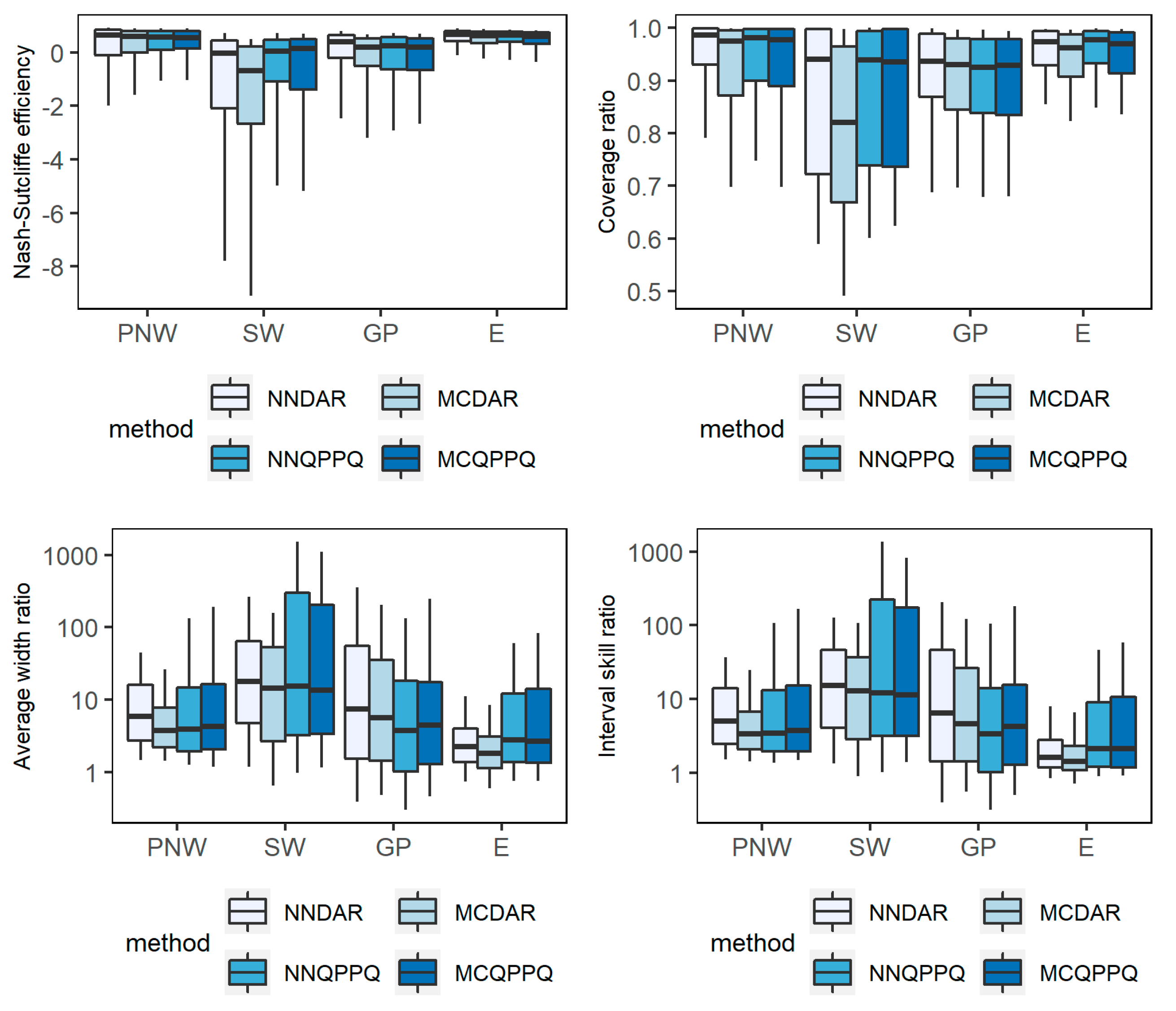
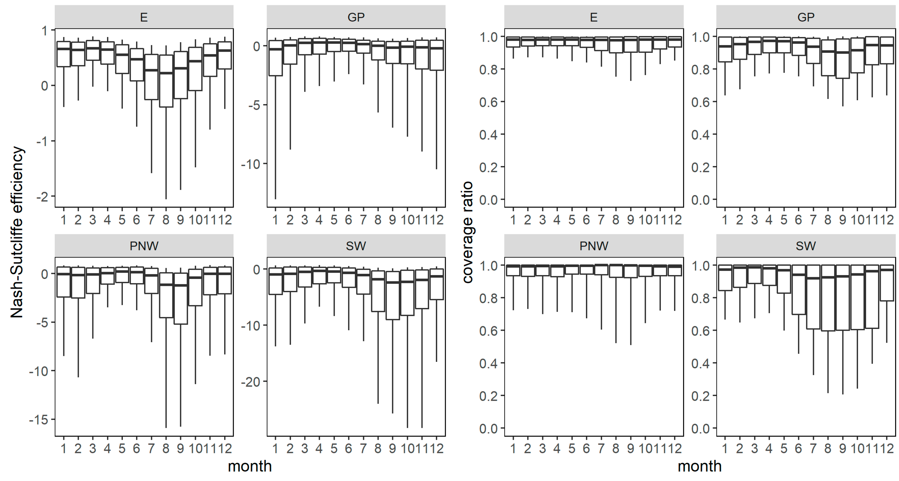
Performance metrics of the validation site simulation and uncertainty intervals developed from all four streamflow methods are shown in Table 1 and Figure 3. Results were grouped into four geographic regions based on level I EPA Eco-regions [29] and similarity of results to facilitate geographic comparisons (Figure 1, Table 1). Overall goodness of fit of the validation site streamflow estimation methods was examined with the NSE [18] (Figure 3, Table 1). The NSE was computed on log-transformed streamflow to reduce oversensitivity to high flows. An NSE of 1.0 indicates that the estimates are identical to the observations; an NSE less than zero indicates that a long-term average value would hold more information than the estimates. Some have suggested that 0.5 be considered an acceptable level for performance in hydrology [30]. Median NSE values for daily streamflows across all validation site simulations were 0.61 and 0.54 for NN- and MC-DAR methods and 0.57 and 0.53 for NN- and MC-QPPQ methods respectively. The median NSE was highest in the Eastern U.S. region, ranging from 0.61 to 0.68, and lowest in the Southwest region, with median values ranging from −0.68 to 0.14 across simulation methods.
Across all sites, median coverage ratios were 0.97 and 0.96 for NN- and MC-DAR methods respectively, and 0.97 for both NN- and MC-QPPQ methods respectively. Median coverage ratios were highest in the Pacific Northwest and mountain region, ranging from 0.97 to 0.99, and in the Eastern U.S. region, ranging from 0.96 to 0.98 (Figure 3). Uncertainty intervals were less reliable in the Great Plains and Southwest regions, particularly for the MCDAR method, which had the lowest median coverage ratio of 0.82. Streamflow simulation and uncertainty interval reliability varied across months in some regions (Figure 4). Month-to-month variability in coverage ratio was minimal in the Eastern U.S. region and moderate in the Pacific Northwest and Great Plains regions. In the Southwest, coverage ratios were less reliable from July through November. Rainfall during these months typically occurs in the form of intense, convective storms that may be spatially fragmented, making it difficult to replicate with statistical methods [31].
The reliability of uncertainty intervals can be affected by bias in the estimated validation streamflow time series. Because the uncertainty intervals are drawn from the pooled errors of 25 separate simulations, the error distributions used to compute the uncertainty intervals are typically distributed fairly evenly around 1 (that is, there are roughly an equal number of over- and under-estimations of first-order donor streamflows). However, at a single target-site simulation, the estimated streamflow time series may contain substantial, systematic bias if the relation between the donor gage and the target stream is poorly characterized by the DAR, or if the flow duration curve is poorly estimated by the regression equations in the QPPQ method. When error ratios from first-order donors are multiplied by biased target-site estimated streamflow values, the uncertainty intervals may also be biased and unreliable. In order to examine the degree to which bias in the validation site estimated streamflow affects the reliability of the uncertainty intervals, the percent bias was computed as:
percent   bias = 100 × ( Q ^ Q o b s ) Q o b s
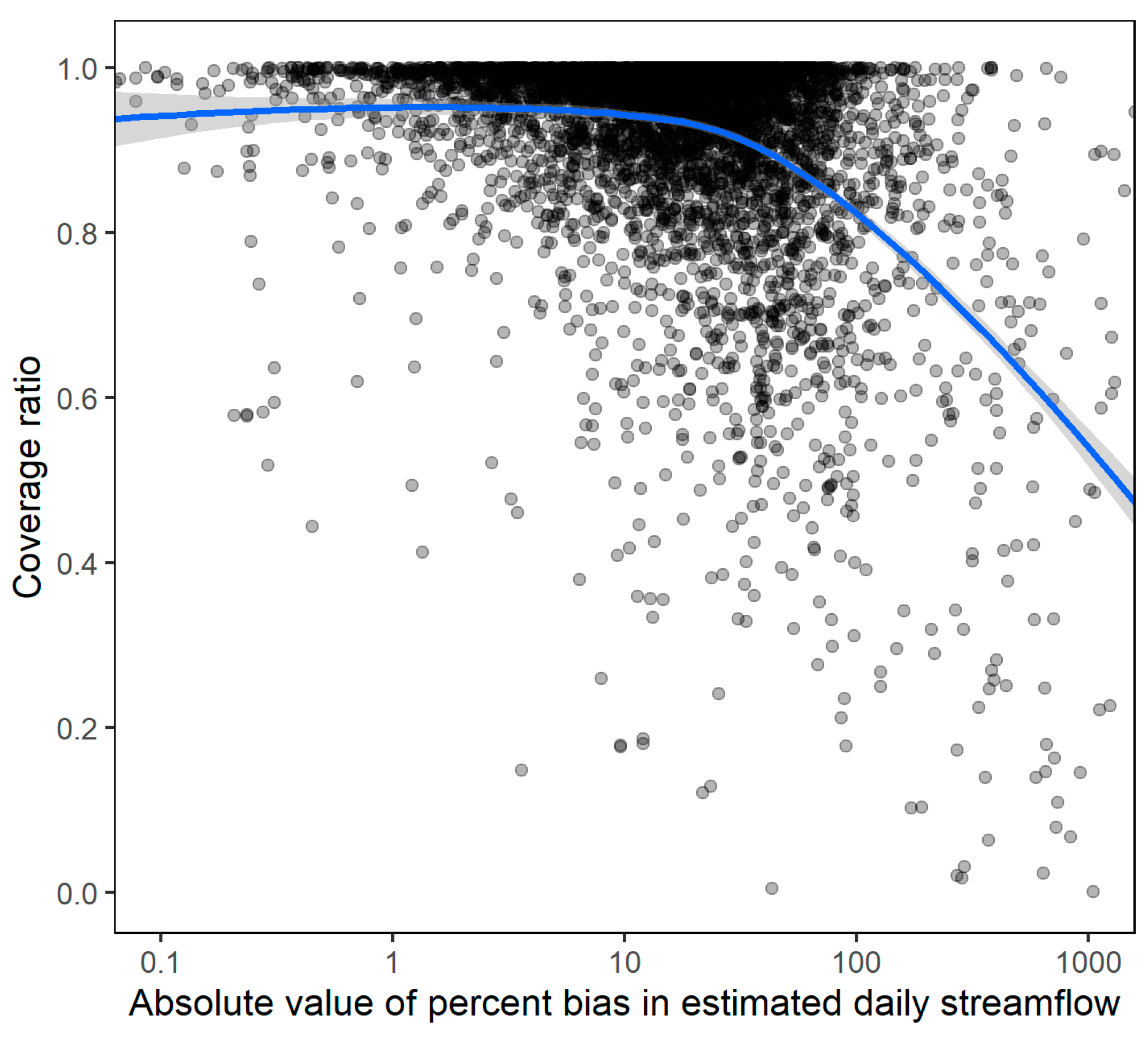
where Q ^ and Q o b s are the estimated and observed daily streamflows. Figure 5 shows that coverage ratios decrease as the percent bias deviates from 0, with average coverage ratios falling below 0.95 when the percent bias deviates from zero by about 10 percent. At a bias greater than ±30 percent, uncertainty intervals may be unreliable, with average coverage ratios below 0.90. The Southwest region had the highest proportion of highly biased validation simulations, with 67 percent of simulations having a percent bias greater than ±30 percent across all four estimation methods. The Great Plains and the Pacific Northwest regions had 45 and 47 percent of simulations with a bias greater than 30 percent, respectively, and the Eastern region had the least biased simulations with only 16 percent of simulations having a bias greater than 30 percent.

3.2. Interval Sharpness

Uncertainty interval widths reflect the regional estimation accuracy; regions with higher accuracy simulations have sharper uncertainty intervals. Uncertainty intervals typically ranged over two or more orders of magnitude compared to the estimated daily streamflow. Intervals were narrowest in the Pacific Northwest and Eastern U.S. regions, which in general had higher accuracy simulations. Median lower bounds in these regions ranged from 0.17 to 0.23 times the estimated streamflow across the four estimation methods, while the median upper bounds ranged from 5.9 to 14.0 times the estimated streamflow. In the Great Plains and Southwest regions, intervals were wider, with median lower bounds ranging from 0.02 to 0.03 and upper bounds ranging from 123 to 261 times the estimated streamflow. Because uncertainty intervals are based on a ratio of streamflows, the relative width of uncertainty intervals (as a percentage of estimated streamflow) were typically widest during low flow periods.
The width of the uncertainty intervals should reflect the level of uncertainty present in the estimated streamflow at the ungaged basin. At a poorly simulated basin, with large errors in daily estimated streamflow, intervals should be wide enough to encompass the magnitude of these estimation errors. In contrast, uncertainty intervals can be narrower while still maintaining an appropriate coverage ratio in well-simulated basins. Therefore, the absolute width of an interval, although useful for application purposes, is not appropriate for assessing the performance of the uncertainty interval. The AWR reflects how well the width of the intervals compares to the actual errors in the validation site simulation. Median AWR values ranged from about 1.8 to 2.7 across the different simulation methods in the Eastern U.S. region, indicating that the intervals in this region are generally of an appropriate width. Median AWR in the Pacific Northwest and Great Plains regions ranged from about 3.7 to 7.4. Interval widths in the Southwest were the largest compared to those produced by the validation site errors, with median AWR values ranging from about 13.5 to 17.8. Intervals in this region are wide compared to the errors within the target site time series.
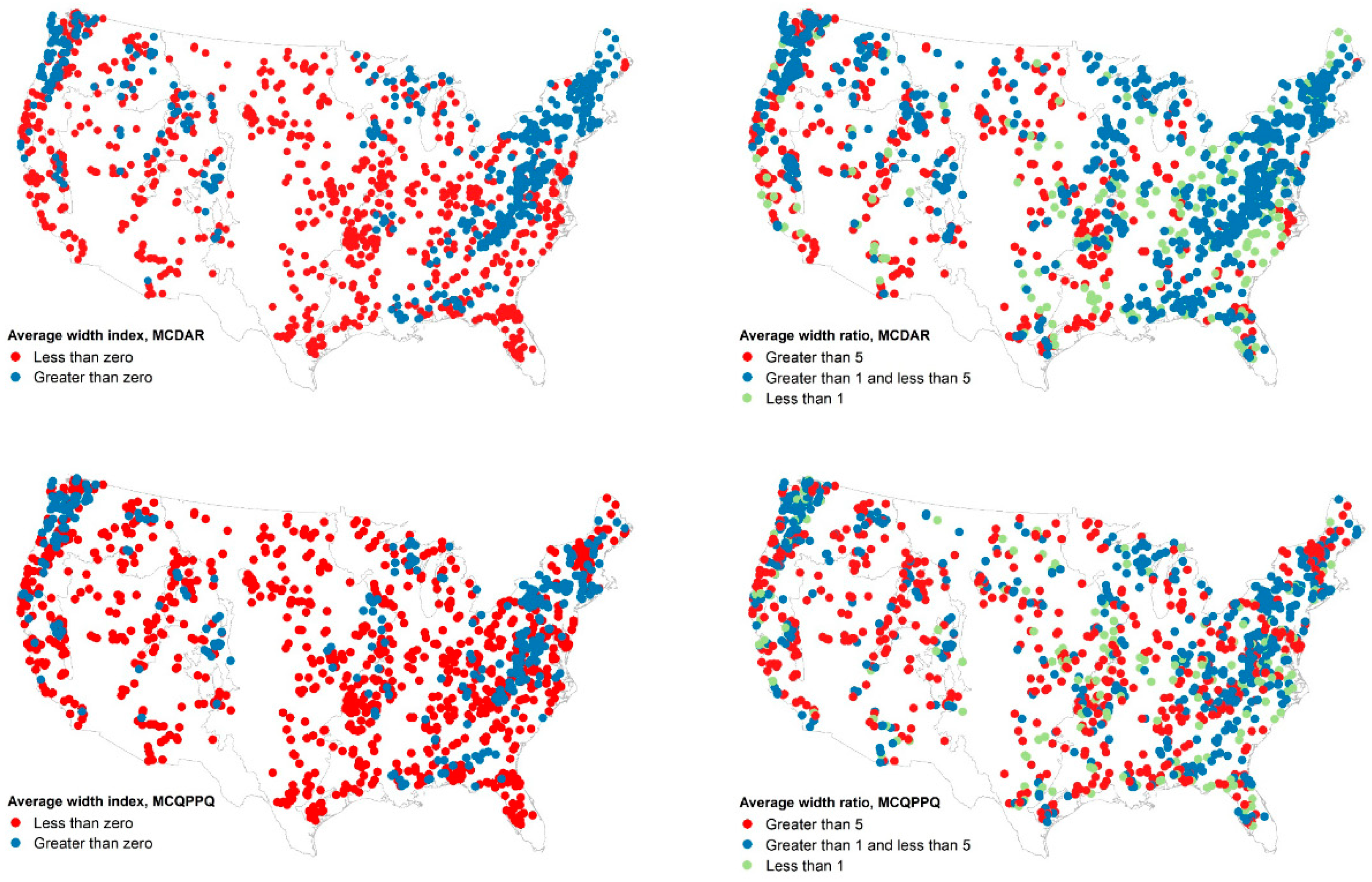
The median AWI was below zero for all methods in the Southwest and Great Plains regions and near zero for all methods in Eastern U.S. and Pacific Northwest regions (Table 1). An AWI below zero indicates that the average width of the uncertainty intervals is wide compared to the overall width of the flow duration curve at the validation site. Figure 6 compares the AWI to the AWR for both MC simulation methods (NN simulations, not shown, were similar to MC simulations). Although the overall spatial patterns of AWI and AWR are similar, there are many locations, particularly in the Eastern U.S. region, where the AWI indicates an overly wide interval (AWI < 0) but where the AWR indicates an appropriate, or even narrow interval (AWR < 5) with respect to the errors at the validation site. Though investigation of physiographic drivers was beyond the scope of this work, results of preliminary analyses indicate that the discrepancies between AWI and AWR tended to align with situations where the region from which donors were drawn crossed some hydrologic barrier (e.g., mountains or shifts in eco-regions) and there was varied performance across this border.
Values for ISR mirrored those of the AWR. Median ISR values in the Eastern U.S. region ranged from about 1.4 to 2.1, reflecting the relatively sharp intervals and high coverage ratios in this region. ISR values were poorest in the Southwest region, with median values ranging from about 11.3 to 15.3 across simulation methods. The large intervals and lower reliability in the Southwest may limit the applicability of the uncertainty intervals in this region. Differences in performance among simulation methods were minor, with the exception of the eastern region, in which the DAR methods produced intervals that were narrower and had higher ISS than the QPPQ methods. Within all regions and methods, there was a high amount of variability in performance, indicating that even in regions with successful overall performance of uncertainty intervals, there are isolated sites which may perform poorly.

3.3. Sensitivity to Regional Factors

The success of the methods used in this paper to characterize uncertainty in DAR and QPPQ methods relies upon the availability of a sufficient number of hydrologically similar donor gages to the ungaged site. Both the hydrologic similarity of a region and the density of streamgages can affect uncertainty interval performance. Streamgage density is important because the procedure to compute uncertainty intervals requires simulations from several hydrologically similar gages. Sparsely gaged areas of the country may not have enough hydrologically similar gaged sites to adequately populate the distribution of relative errors. Hydrologic similarity is important because information regarding the timing and magnitude of streamflow and, for the DAR method, the magnitude of streamflows, is transferred from an index gage and sites that are highly correlated produce more accurate simulations [32]. Additionally, if there are few highly correlated index gages at a particular ungaged location, then the error ratios produced in the uncertainty estimation procedure may not adequately match those of the target site simulation.
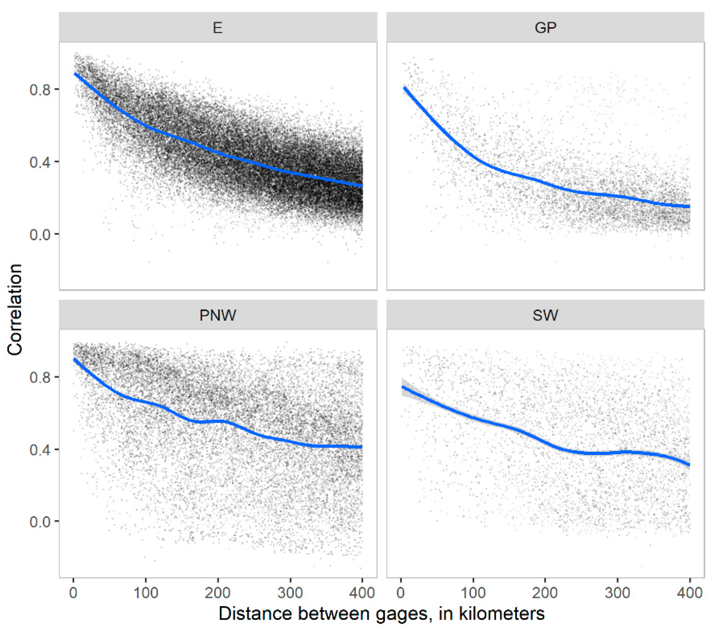
Regional differences in simulation and uncertainty interval performance may be influenced by the relation between distance and correlation between gages (Figure 7). The eastern region is densely gaged, with a median of 105 gages per 500,000 km2. Additionally, the relation between correlation and distance has less variability than other regions. Sites in this region had high NSE and coverage ratios, and also showed less variability in results than in other regions. The relation between distance and gage correlation in the Great Plains is similar to that of the Eastern region, except that the gage density is the lowest of the four regions, with a median gage density of 46 gages per 500,000 km2. Variability in the NSE values and uncertainty interval performance may result from the sparseness of the gage network in this region. The low gage density necessitates using gages from further away, with a potentially lower correlation to the target site in order to perform the uncertainty interval procedure. The Pacific Northwest region has the second highest gage density, with a median of 82 gages per 500,000 km2. However, there is high variability in gage correlation, even at close distances. In this region, although there are typically plenty of potential index gages nearby to choose from, the high level of variability increases the chance that a given simulation will select an index gage with a poor correlation to the target site. The increased heterogeneity in this region may explain the increased variance in the NSE and coverage ratios. Finally, the Southwest region has a low gage density, with a median of 48 gages per 500,000 km2 and also has a high amount of variability in gage correlation, resulting in lower overall performance of validation site simulations and uncertainty intervals.
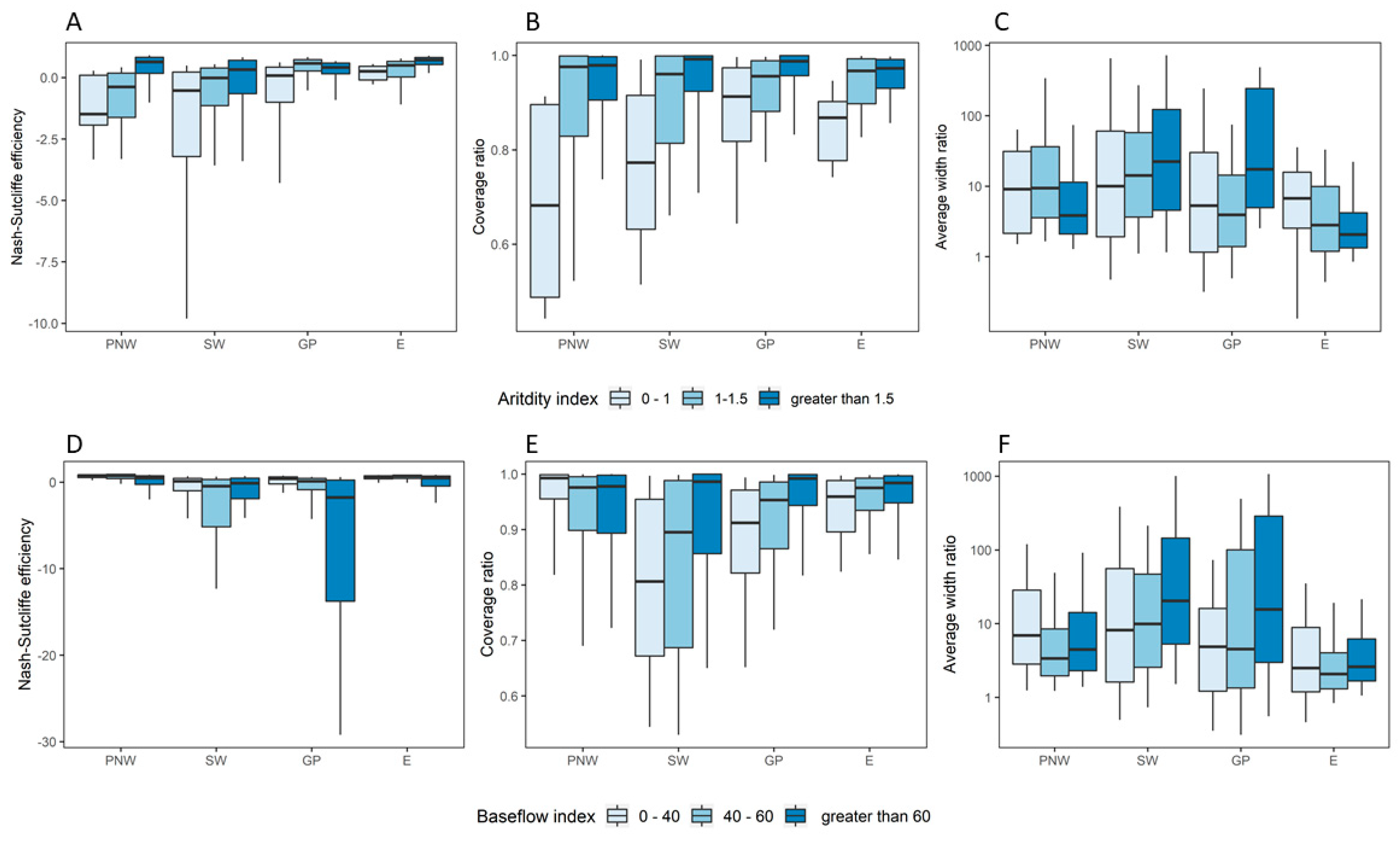
The hydroclimatic regime defines the relative predominance and seasonal patterns of evaporative or precipitation processes within a basin. Hydroclimatic and physical basin characteristics have been used to classify catchments with similar hydrologic signatures and to explain the performance of streamflow estimation. Singh et al. [33] found that across the continental United States, similarity in climate, soil, and land use characteristics were among the dominant basin characteristics that resulted in the best parameter transfer in a calibrated rainfall runoff model. Patil and Stieglitz [32] found that NSE of DAR-based streamflow estimation methods were higher in humid basins. The aridity index [34] was computed as the average annual precipitation/potential evapotranspiration (PET) for all basins. Across regions, lower aridity index (drier) was correlated with poorer NSE and coverage ratios (Figure 8). Uncertainty intervals were generally unreliable, with median coverage ratios below 0.95, in basins where the aridity index was less than one. In these basins, the mean annual PET exceeds annual precipitation. Baseflow index is a measure of the percentage of streamflow that is from baseflow. Within each region, baseflow dominated streams (baseflow index > 60%) generally had lower NSE than runoff-dominated streams but had higher coverage ratios and average width ratios (Figure 8). One potential reason for this result is that baseflow-dominated streams tend to have lower streamflow variability because of the relatively steady contribution of groundwater. If surrounding index gages do not share this high baseflow index, then the target simulation will likely have large errors and a low NSE. Additionally, in areas where the surrounding index gages are poorly simulated, uncertainty intervals will be wide and the low variability of the observed streamflow at the target site will lead to fewer observations outside the uncertainty intervals, leading to high coverage ratios.
While climate, baseflow, gage density, and hydrologic similarity explain some of the variability in the performance of the uncertainty intervals, there is no one basin characteristic that fully explains it. Even in regions with generally good at-site simulation and uncertainty characterization, there are outlying sites where the methods do not perform well. Patil and Steiglitz [32] suggest that while regional performance of streamflow simulation methods may be explained by large scale variability in climate, geology, or other physical features, low performance at a specific site may be attributed to smaller scale climate variability or idiosyncratic hydrologic behavior at the site that is not representative of the surrounding areas.

4. Conclusions

A method to produce empirical uncertainty intervals around daily estimated streamflows for four transfer-based estimation methods was tested across the conterminous United States. Uncertainty intervals at a target site were produced by transferring relative errors of estimated streamflow at hydrologically similar gaged sites for 1331 streamgages. Uncertainty intervals were evaluated using the coverage ratio, average width ratio, and interval skill ratio, which quantify the reliability, sharpness, and overall interval skill, respectively. Coverage ratios performed best in the Eastern U.S. region, with median coverage ratios ranging from 0.96 to 0.98 across four simulation methods. Median average width ratios ranged from 1.8 to 2.7. Uncertainty intervals in the Eastern U.S. region were reliable and the interval widths closely matched the magnitude of error ratios in the estimated streamflow time series at the target site. Intervals in the Pacific Northwest and Great Plains regions had median coverage ratios ranging from 0.92 to 0.99 across methods, and median AWR in these regions ranged from 3.7 to 7.4. Intervals in the Southwest performed the poorest, with median coverage ratios ranging from 0.82 to 0.94 and median AWR values ranging from 13.5 to 17.8. Intervals in this region were very large compared to the magnitude of error ratios present in the estimated streamflow time series. This lack of precision combined with low reliability, may make uncertainty intervals unsuitable for use in this region.
Uncertainty interval performance is associated with the correlation among nearby index gages and gage density. The Eastern region benefits from a very dense gage network combined with a high correlation among nearby gages. This makes it possible to find a highly correlated index gage for the target site simulation and an adequate number of similar index gages for use in the uncertainty interval estimation process. The Pacific Northwest region is very densely gaged, but there is considerable variability in the correlation between nearby gages. Thus, although there are a large number of index gages to choose from, the inclusion of index gages that are poorly correlated to the target site may reduce the NSE at the target site or the performance of the uncertainty intervals. Simulations and uncertainty interval estimation in this region may benefit from more sophisticated screening of potential index gages than was used in this study. The Great Plains and Southwest regions have a lower density of gages and lower overall correlation between gages, resulting in overall poorer and more variable performance of streamflow simulations and uncertainty interval performance in these regions. Within each region, simulation accuracy and uncertainty interval performance showed some sensitivity to the aridity index and the baseflow index. Sites with higher aridity index (wetter conditions) had higher NSE and more reliable intervals and sites. Sites with higher baseflow contributions had lower NSE and as good or better coverage ratios than other validation sites within the same region.

Author Contributions

Conceptualization, S.B.L. and W.H.F.; methodology, S.B.L.; software, S.B.L.; validation, S.B.L.; formal analysis, S.B.L.; investigation, S.B.L.; resources, S.B.L and W.H.F.; data curation, S.B.L.; writing—original draft preparation, S.B.L.; writing—review and editing, S.B.L. and W.H.F.; visualization, S.B.L.; supervision, W.H.F.; project administration, W.H.F.; funding acquisition, W.H.F. All authors have read and agreed to the published version of the manuscript.

Funding

This work was funded by the U.S. Geological Survey’s National Water Census, a part of the Water Availability and Use Science Program

Acknowledgments

The authors acknowledge the support of the Water Budget Estimation and Evaluation project. We also greatly appreciate the contributions of anonymous reviewers that considered early versions of the manuscript. Upon acceptance of this work, a complete archive of the data and models used herein is available in Levin [23]; https://doi.org/10.5066/P9KCLD9W. Any use of trade, firm, or product names is for descriptive purposes only and does not imply endorsement by the U.S. Government.

Conflicts of Interest

The authors declare no conflict of interest.

References

  1. Kennedy, K.; Lutz, K.; Hatfield, C.; Martin, L.; Barker, T.; Kennedy, K.; Palmer, R.; Detwiler, L.; Anleitner, J.; Hickey, J. The Connecticut River Flow Restoration Study: A Watershed-Scale Assessment of the Potential for Flow Restoration Through Dam Re-Operation; The Nature Conservancy, U.S. Army Corps of Engineers, and University of Massachusetts: Northampton, MA, USA, 2018. [Google Scholar]
  2. Poff, N.L.; Richter, B.D.; Arthington, A.H.; Bunn, S.E.; Naiman, R.J.; Kendy, E.; Acreman, M.; Apse, C.; Bledsoe, B.P.; Freeman, M.C.; et al. The ecological limits of hydrologic alteration (ELOHA): A new framework for developing regional environmental flow standards: Ecological limits of hydrologic alteration. Freshw. Biol. 2010, 55, 147–170. [Google Scholar] [CrossRef] [Green Version]
  3. Richter, B.D.; Mathews, R.; Harrison, D.L.; Wigington, R. Ecologically sustainable water management: Managing river flows for ecological integrity. Ecol. Appl. 2003, 13, 206–224. [Google Scholar] [CrossRef]
  4. Weiskel, P.K.; Brandt, S.L.; DeSimone, L.A.; Ostiguy, L.J.; Archfield, S.A. Indicators of Streamflow Alteration, Habitat Fragmentation, Impervious Cover, and Water Quality for Massachusetts Stream Basins; Scientific Investigagions Report 2009-5272; U.S. Geological Survey: Reston, VA, USA, 2009. [Google Scholar]
  5. Shu, C.; Ouarda, T.B.M.J. Improved methods for daily streamflow estimates at ungauged sites. Water Resour. Res. 2012, 48. [Google Scholar] [CrossRef]
  6. Hirsch, R.M. An evaluation of some record reconstruction techniques. Water Resour. Res. 1979, 15, 1781–1790. [Google Scholar] [CrossRef]
  7. Gianfagna, C.C.; Johnson, C.E.; Chandler, D.G.; Hofmann, C. Watershed area ratio accurately predicts daily streamflow in nested catchments in the Catskills, New York. J. Hydrol. Reg. Stud. 2015, 4, 583–594. [Google Scholar] [CrossRef] [Green Version]
  8. Asquith, W.H.; Roussel, M.C.; Vrable, J. Statewide Analysis of the Drainage-Area Ratio Method for 34 Streamflow Percentile Ranges in Texas; Scientific Investigations Report 2006-5286; U.S. Geological Survey: Reston, VA, USA, 2006; p. 34. [Google Scholar]
  9. Emerson, D.G.; Vecchia, A.V.; Dahl, A.L. Evaluation of Drainage Area Ratio Method Used to Estimate Streamflow for the Red River of the North Basin, North Dakota and Minnesota; Scientific Investigations Report; U.S. Geological Survey: Reston, VA, USA, 2005; p. 13. [Google Scholar]
  10. Ries III, K.G.; Friesz, P.J. Methods for Estimating Low-Flow Statistics for Massachusetts Streams; Water-Resources Investigations Report 00-4135; U.S. Geological Survey: Reston, VA, USA, 2000. [Google Scholar]
  11. Fennessey, N.M. A Hydro-Climatological Model of Daily Streamflow for the Northeast United States. Ph.D. Thesis, Tufts University, Medford, MA, USA, 1994. [Google Scholar]
  12. Smakhtin, V.Y. Generation of natural daily flow time-series in regulated rivers using a non-linear spatial interpolation technique. Regul. Rivers Res. Manag. 1999, 15, 311–323. [Google Scholar] [CrossRef]
  13. Mohamoud, Y.M. Prediction of daily flow duration curves and streamflow for ungauged catchments using regional flow duration curves. Hydrol. Sci. J. 2008, 53, 706–724. [Google Scholar] [CrossRef]
  14. Archfield, S.A.; Vogel, R.M.; Steeves, P.A.; Brandt, S.L.; Weiskel, P.K.; Garabedian, S.P. The Massachusetts Sustainable-Yield Estimator: A Decision-Support Tool to Assess Water Availability at Ungaged Stream Locations in Massachusetts; Scientific Investigations Report 2009-5227; U.S. Geological Survey: Reston, VA, USA, 2010. [Google Scholar]
  15. Lorenz, D.L.; Ziegeweid, J.R. Methods to Estimate Historical Daily Streamflow for Ungaged Stream Locations in Minnesota; Scientific Investigations Report 2015-5181; U.S. Geological Survey: Reston, VA, USA, 2016. [Google Scholar]
  16. Gazoorian, C.L. Estimation of Unaltered Daily Mean Streamflow at Ungaged Streams of New York, Excluding Long Island, Water Years 1961–2010; Scientific Investigations Rerpot 2014-5220; U.S. Geological Survey: Reston, VA, USA, 2015; p. 29. [Google Scholar]
  17. Stuckey, M.H.; Koerkle, E.H.; Ulrich, J.E. Estimation of Baseline Daily Mean Streamflows for Ungaged Locations on Pennsylvania Streams, Water Years 1960-2008; Scientific Investigations Report; U.S. Geological Survey: Reston, VA, USA, 2012; p. 68. [Google Scholar]
  18. Nash, J.E.; Sutcliffe, J.V. River flow forecasting through conceptual models part I—A discussion of principles. J. Hydrol. 1970, 10, 282–290. [Google Scholar] [CrossRef]
  19. Fry, L.M.; Hunter, T.S.; Phanikumar, M.S.; Fortin, V.; Gronewold, A.D. Identifying streamgage networks for maximizing the effectiveness of regional water balance modeling: Identifying Gage Networks. Water Resour. Res. 2013, 49, 2689–2700. [Google Scholar] [CrossRef]
  20. Bourgin, F.; Andréassian, V.; Perrin, C.; Oudin, L. Transferring global uncertainty estimates from gauged to ungauged catchments. Hydrol. Earth Syst. Sci. 2015, 19, 2535–2546. [Google Scholar] [CrossRef]
  21. Farmer, W.H.; Levin, S. Characterizing Uncertainty in Daily Streamflow Estimates at Ungauged Locations for the Massachusetts Sustainable Yield Estimator. J. Am. Water Resour. Assoc. 2018, 54, 198–210. [Google Scholar] [CrossRef]
  22. Falcone, J.A.U.S. Geological Survey GAGES-II Time Series Data from Consistent Sources of Land Use, Water Use, Agriculture, Timber Activities, Dam Removals, and Other Historical Anthropogenic Influences; U.S. Geological Survey: Reston, VA, USA, 2017. [Google Scholar]
  23. Levin, S.B. Performance Metrics for 95-Percent Confidence Intervals of Estimated Daily Streamflow Using Four Transfer-Based Simulation Methods Across the Continental U.S.; U.S. Geological Survey Data Release. Available online: https://www.sciencebase.gov/catalog/item/5e861895e4b01d50927fb74a (accessed on 1 May 2020).
  24. Over, T.M.; Farmer, W.H.; Russell, A.M. Refinement of a Regression-Based Method for Prediction of Flow-Duration Curves of Daily Streamflow in the Conterminous United States; Scientific Investigations Report 2018-5072; U.S. Geological Survey: Reston, VA, USA, 2018; p. 44. [Google Scholar]
  25. Archfield, S.A.; Vogel, R.M. Map correlation method: Selection of a reference streamgage to estimate daily streamflow at ungaged catchments. Water Resour. Res. 2010, 46. [Google Scholar] [CrossRef]
  26. Andréassian, V.; Lerat, J.; Le Moine, N.; Perrin, C. Neighbors: Nature’s own hydrological models. J. Hydrol. 2012, 414–415, 49–58. [Google Scholar]
  27. Bock, A.R.; Farmer, W.H.; Hay, L.E. Quantifying uncertainty in simulated streamflow and runoff from a continental-scale monthly water balance model. Adv. Water Resour. 2018, 122, 166–175. [Google Scholar] [CrossRef]
  28. Gneiting, T.; Raftery, A.E. Strictly Proper Scoring Rules, Prediction, and Estimation. J. Am. Stat. Assoc. 2007, 102, 359–378. [Google Scholar] [CrossRef]
  29. US Environmental Protection Agency, Office of Research and Development. Ecoregions of North America. Available online: https://www.epa.gov/eco-research/ecoregions-north-america (accessed on 16 March 2020).
  30. Moriasi, D.N.; Arnold, J.G.; Van Liew, M.W.; Bingner, R.L.; Harmel, R.D.; Veith, T.L. Model Evaluation Guidelines for Systematic Quantification of Accuracy in Watershed Simulations. Trans. ASABE 2007, 50, 885–900. [Google Scholar] [CrossRef]
  31. Adams, D.K.; Comrie, A.C. The North American Monsoon. Bull. Am. Meteorol. Soc. 1997, 78, 2197–2214. [Google Scholar] [CrossRef] [Green Version]
  32. Patil, S.; Stieglitz, M. Controls on hydrologic similarity: Role of nearby gauged catchments for prediction at an ungauged catchment. Hydrol. Earth Syst. Sci. 2012, 16, 551–562. [Google Scholar] [CrossRef] [Green Version]
  33. Singh, R.; Archfield, S.A.; Wagener, T. Identifying dominant controls on hydrologic parameter transfer from gauged to ungauged catchments—A comparative hydrology approach. J. Hydrol. 2014, 517, 985–996. [Google Scholar] [CrossRef]
  34. Middleton, N.; Thomas, D. World Atlas of Desertification; UNEP: Nairobi, Kenya, 1997; ISBN 0340691662. [Google Scholar]
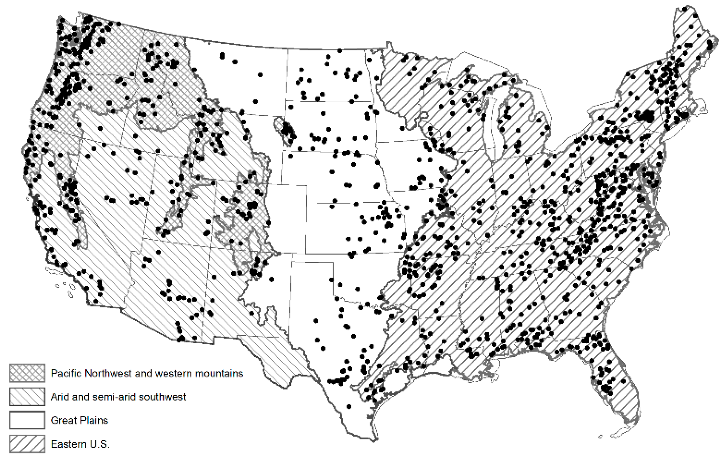
Figure 1. Locations of 1331 U.S. Geological Survey streamgages used as validation sites, and regions used for grouping study results.
Water 12 01390 g001
Figure 2. Schematic diagram of the process used to compute uncertainty intervals for daily streamflows. First order index gages are selected (A) and simulated as if they were ungaged using 5 second -order index gages (B). Daily error ratios are grouped by month (C). Confidence intervals are computed by multiplying the daily estimated streamflow at the ungaged site by the 97.5 and 2.5 percentile error ratios of the appropriate month.
Water 12 01390 g002
Figure 3. Distribution of streamflow simulation and uncertainty intervals performance for 1331 validation streamgage sites in four regions: Pacific Northwest and mountains (PNW), Southwest (SW), Great Plains (GP), and Eastern U.S. (E). Boxplot whiskers extend to the 10th and 90th percentiles of the distribution, box ends represent the 25th and 75th percentiles, and the horizontal line represents the median.
Water 12 01390 g003
Figure 4. Monthly Nash–Sutcliffe efficiency of daily streamflow simulations and coverage ratio of 95 percent uncertainty intervals in four regions in the study area: Eastern U.S. (E), Great Plains (GP), Pacific Northwest and mountains (PNW), and Southwest (SW). Boxplot whiskers extend to the 10th and 90th percentiles of the distribution, box ends represent the 25th and 75th percentiles, and the horizontal line represents the median.
Water 12 01390 g004
Figure 5. Absolute value of the percentage bias of daily streamflow time series and the coverage ratio associated with 95 percent uncertainty intervals of the streamflow time series. Blue line is a smoothed conditional mean.
Water 12 01390 g005
Figure 6. Average width index (AWI) and average width ratio (AWR) for 95 percent uncertainty intervals at 1331 validation sites using MCDAR and MCQPPQ simulation methods.
Water 12 01390 g006
Figure 7. Distance between streamgages and correlation in daily streamflow for four regions in the study area: Eastern U.S. (E), Great Plains (GP), Pacific Northwest and mountains (PNW), and Southwest (SW). Blue line is a smoothed conditional mean.
Water 12 01390 g007
Figure 8. Nash–Sutcliffe efficiency of daily streamflow estimates and coverage ratio and average width index (AWI) of 95 percent uncertainty intervals, grouped by aridity index (AC) and baseflow index (DE) at 1331 validation sites in four regions of the study area: Pacific Northwest and mountains (PNW), Southwest (SW), Great Plains (GP), and Eastern U.S. (E). Boxplot whiskers extend to the 10th and 90th percentiles of the distribution, box ends represent the 25th and 75th percentiles, and the horizontal line represents the median.
Water 12 01390 g008
Table 1. Quantiles of performance metrics for simulation and uncertainty intervals of daily streamflow four simulation methods in four regions: Pacific Northwest and mountains (PNW), Southwest (SW), Great Plains (GP), and Eastern U.S. (E). Simulation methods include drainage area ratio using nearest neighbor index gage selection (NNDAR) and map correlation selection methods (MCDAR) and nonlinear spatial interpolation using flow duration curves (QPPQ) using nearest neighbor index gage selection (NNQPPQ) and map correlation index gage selection (MCQPPQ).
MetricRegionNumber of SitesQuantiles of Metrics for NNDARQuantiles of Metrics for MCDAR
1%5%25%50%75%95%99%1%5%25%50%75%95%99%
NSEPNW319−10−4.2−0.140.650.850.940.98−10−3.5−0.010.590.800.940.97
SW123−44−16−2.2−0.020.460.820.91−63−21−2.7−0.680.230.720.82
GP161−25−8.7−0.190.400.660.840.86−81−11−0.520.210.530.780.85
E728−7.8−0.990.430.680.810.930.97−5.9−1.10.340.630.770.900.94
CRPNW3190.440.640.930.991.01.01.00.100.490.870.971.01.01.0
SW1230.150.460.720.941.01.01.00.110.350.670.820.961.01.0
GP1610.250.580.870.940.991.01.00.110.600.850.930.981.01.0
E7280.640.790.930.970.991.01.00.570.750.910.960.991.01.0
AWRPNW3190.160.912.75.8169317600.321.12.23.77.8107626
SW1230.180.684.7186552820800.050.252.714544496850
GP1610.020.231.17.45555831100.020.241.45.63578117,100
E7280.080.331.42.24.0251860.070.201.11.83.118113
ISRPNW3190.301.22.45.1146514700.631.22.063.36.782559
SW1230.310.834.0154731719300.060.382.813383045070
GP1610.020.231.46.54648419500.020.241.44.6264922840
E7280.080.361.21.62.8191040.070.231.11.42.31451
AWIPNW319−434−40−5.8−1.10.250.640.75−287−59−1.6−0.220.400.690.79
SW123−1590−714−75−18−5.70.070.36−9000−1480−62−13−1.70.340.69
GP161−3380−819−121−24−6.6−1.10.43−21,800−1510−103−28−6.7−0.280.63
E728−104−35−2.4−0.120.30.550.64−99−35−2.1−0.020.390.620.70
ISSPNW319−340−27−3.5−0.450.390.700.78−211−36−1.40.060.490.740.79
SW123−1100−204−27−9.2−2.50.230.51−3280−388−23−5.3−1.10.350.62
GP161−1960−413−46−8.8−1.90.130.53−3830−607−32−10−1.90.280.66
E728−48−14−0.810.300.550.690.75−49−16−0.770.280.560.720.77
NSEPNW319−9.1−2.60.080.570.800.920.95−9.3−3.10.150.560.810.910.96
SW123−18−9.5−1.20.060.490.830.87−16−9.6−1.50.140.490.800.84
GP161−47−7.2−0.630.260.570.820.86−29−7.6−0.660.200.530.760.84
E728−4.0−0.970.400.640.780.890.93−3.9−1.20.330.610.750.870.92
CRPNW3190.380.620.900.981.01.01.00.260.540.890.981.01.01.0
SW1230.340.510.730.940.991.01.00.450.570.730.941.01.01.0
GP1610.390.640.840.920.981.01.00.420.600.840.930.981.01.0
E7280.410.790.930.980.991.01.00.380.750.910.970.991.01.0
AWRPNW3190.450.881.93.91578853800.420.822.034.217140037,600
SW1230.220.383.115373320027,4000.170.463.2314220326032,800
GP1610.060.151.03.71873926,9000.030.301.34.518109022,400
E7280.110.411.342.7122179660.150.451.32.714247815
ISRPNW3190.931.22.03.41464738200.931.22.03.715117029,000
SW1230.230.443.112228189026,5000.200.493.111186187026,100
GP1610.090.201.03.41463723,7000.040.321.234.3158925750
E7280.120.511.22.19.01288090.200.611.22.111192612
AWIPNW319−1540−482−4.8−0.550.350.670.75−13,100−826−6.3−0.690.350.690.79
SW123−29,200−3360−414−22−3.80.290.51−15,000−3800−371−30−5.80.090.63
GP161−45,700−2260−88−16−3.9−0.220.60−42,000−2060−127−27−4.70.150.70
E728−635−138−9.6−0.960.220.570.67−621−216−13−1.10.180.580.66
ISSPNW319−1090−281−3.3−0.130.450.710.76−8670−508−4.2−0.320.430.700.77
SW123−23,800−1500−151−9.0−1.60.610.70−12,000−1270−134−17−1.70.430.60
GP161−20,900−576−31−5.6−0.840.430.56−9300−824−45−9.9−1.20.400.55
E728−316−73−4.8−0.170.490.690.75−286−111−6.3−0.250.440.680.75