Article

Application of Random Forest and ICON Models Combined with Weather Forecasts to Predict Soil Temperature and Water Content in a Greenhouse

1
Department of Bioenvironmental Systems Engineering, National Taiwan University, Taipei 10617, Taiwan
2
Department of Horticulture and Landscape Architecture, National Taiwan University, Taipei 10617, Taiwan
*
Author to whom correspondence should be addressed.
Water 2020, 12(4), 1176; https://doi.org/10.3390/w12041176
Submission received: 20 March 2020 / Revised: 14 April 2020 / Accepted: 16 April 2020 / Published: 20 April 2020
(This article belongs to the Section Hydrology)

Abstract

:
Climate change might potentially cause extreme weather events to become more frequent and intense. It could also enhance water scarcity and reduce food security. More efficient water management techniques are thus required to ensure a stable food supply and quality. Maintaining proper soil water content and soil temperature is necessary for efficient water management in agricultural practices. The usage of water and fertilizers can be significantly improved with a precise water content prediction tool. In this study, we proposed a new framework that combines weather forecast data, numerical models, and machine learning methods to simulate and predict the soil temperature and volumetric water content in a greenhouse. To test the framework, we performed greenhouse experiments with cherry tomatoes. The numerical models and machine learning methods we selected were Newton’s law of cooling, HYDRUS-1D, the random forest model, and the ICON (inferring connections of networks) model. The measured air temperature, soil temperature, and volumetric water content during the cultivation period were used for model calibration and validation. We compared the performances of the models for soil temperature and volumetric water content predictions. The results showed that the random forest model performed a more accurate prediction than other methods under the limited information provided from greenhouse experiments. This approach provides a framework that can potentially learn best water management practices from experienced farmers and provide intelligent information for smart greenhouse management.

1. Introduction

Given the vulnerability of agricultural production to extreme weather events whose intensity and frequency will increase with climate change, proactively managing agricultural risks to sustain production is becoming increasingly important [1]. To ensure a stable food supply and quality, intensive farming has been used since the mid-1980s to monitor the food production chain and manage its supply and quality. Precision agriculture can optimize crop/fruit production while maintaining environmental quality to achieve a safe food supply [2]. Precision agriculture includes a range of technologies, including enhanced sensors, information systems, and mechanical equipment. This approach primarily optimizes production efficiency by considering and managing uncertainty and variability within agricultural systems [3]. Compared with a field cultivation system, precision agriculture is relatively easy to achieve in a greenhouse system because it can control environmental factors more effectively.
Greenhouse systems can ensure the quality of crops by saving water, controlling the temperature and reducing the use of pesticides [4]. Placing the monitoring instruments in a greenhouse can also enhance management effectiveness [5]. Moreover, for plants, root development will affect future growth [6]. Soil temperature and water content are closely related to the root systems of plants. Water content can provide protection for plant root systems and reduce changes in soil temperature caused by changes in air temperature between day and night [7]. However, previous studies have noted that even if a greenhouse system compared to outdoors can control many environmental factors, there are still many uncontrollable conditions and interactions [8]. These factors cause difficulties in maintaining soil temperature and water content for efficient water management and plant root protection in agricultural practices. To achieve this aim, the management of optimized soil temperature and water content in a greenhouse system still needs to be improved. Therefore, it is necessary to develop a framework for intelligent prediction.
To understand the relationship between soil temperature and water content, the interactions between water content and heat in soil have been explored [9,10,11]. Later, HYDRUS-1D was developed as a simulation software that combined thermal diffusion and the Richards’ equation [12]. However, the soil parameters required for simulation must be measured by various complex and time-consuming experiments, thus, data-based mathematical models have recently emerged. Machine learning techniques have become a popular data-based mathematical model in recent years. Machine learning is a method used to teach machines how to handle data more efficiently when it is difficult to interpret patterns or extract information from data [13,14]. Without knowing the actual physical mechanisms involved, using a data-based mathematical model to train data can produce predictions of unknown generation criteria [13]. Machine learning techniques have been used to simulate large-scale soil water content [15,16] and have been compared with numerical methods in the simulation differences of soil water content [17]. However, machine learning has not been used to predict the change trends of soil water content from temperature. Through the inseparable relationship between soil water content and soil temperature [9,12], we can apply machine learning to predict the change of water content over time. Moreover, compared with machine learning, dynamic topology provides an ICON (inferring connections of networks) model to simulate the trend of time series data, uses the existing data to build the system, and determines the relationship between various factors in the system [18]. The ICON model was proposed by Wang et al., 2018 with the aim to extract complex interactions in natural systems in which multiple factors affect each other dynamically. ICON is also a data-driven approach of dynamic interactions for determining the network topology of oscillators with different coupling functions, periodicities, degree nodes, and time scales through solving nonlinear estimation problems as a linear inverse problem [18]. This model can depict the dynamic interactions of a large complex system with noisy data in various fields. Both ICON and machine learning techniques can make predictions without first obtaining physical parameters, which is highly suitable for the dynamic interactions of complex impact factors.
Previous studies focused on simulations but failed to provide future predictions [15,16,17]. In a greenhouse where the temperature cannot be controlled, the indoor temperature is related to the outdoor temperature and weather. Through this relationship, it is possible to use the weather forecast data to predict the soil temperature and water content in a greenhouse [4,19]. Therefore, the objective of this study is to provide a framework for predicting soil temperature and water content based on a weather forecast with limited measured information. In this study, we also compared the prediction performance of different types of models. We used the monitoring instruments and sensors to collect long-term time-series data for model calibration and validation. The soil temperature and water content were simulated and predicted by combining the weather forecast data. Our findings can improve the usage of water, accurately assess water requirements under various temperature effects, and further develop water content and temperature alarms for greenhouse management.
The greenhouse environment and the characteristics of the materials are described in Section 2. We also detail the methodology of the analyses’ data processes. In Section 3, the related applied physics theories and numerical models are introduced. Section 4 is dedicated to the results of the temporal distribution of air and soil temperatures, and the volumetric water content (VWC) for cherry tomato growth. Moreover, we discuss the simulation results and the performances from the models and predict the future soil temperature and water content by combining the weather forecast data. The conclusion is presented in Section 5.

2. Materials and Methods

2.1. Greenhouse Setup

Our experiments were performed in a greenhouse (24 meters long, 9.6 meters wide, and 5.5 meters high) with a pad and fan system at NTU (National Taiwan University, Taipei, Taiwan). We used the HOBO U23 Pro v2 Temperature/Relative Humidity Data-logger (Onset Computer Corp., Bourne, MA, USA; accuracy: temperature ± 0.2 °C, relative humidity ± 2.5%; range: temperature −40 to 70 °C, relative humidity 0 to 100%) to collect air temperature and relative humidity in the greenhouse during the experiments. At the same time, the monitoring instruments and sensors were installed. These instruments included 5TE sensors (Decagon Devices, Inc., WA, USA; accuracy: VWC ± 0.03 m3 m−3, soil temperature ± 1 °C; range: VWC 0 to 1 m3 m−3, soil temperature −40 to 50 °C), temperature probes (T-type Thermocouple, Nzing Co., Taiwan; accuracy: temperature ± 1 °C; range: −200 to 200 °C), HFT-3 heat flux transducers (Campbell Scientific, Inc., UT, USA; accuracy: better than ± 5% of reading; range: −100 to 100 W m−2; thermal conductivity 1.22 W m−1 K−1), 2100F tensiometers and Model 5301 current transducers (Soilmoisture Equipment Corp., CA, USA; accuracy: matric potential ± 1% span; range: 2 bar pressure difference), T5 pressure transducer tensiometers (UMS GmbH, München, Germany; accuracy: matric potential ± 0.5 kPa; range: −85 to 100 kPa), and the CR1000 data-logger (Campbell Scientific, Inc., UT, USA) for real-time and long-term monitoring of soil water content, soil temperature, soil heat flow, electrical conductivity, and soil matric potential (suction) in the greenhouse. Moreover, before installing the sensors, an inspection process had been completed to ensure that each sensor satisfied the manufacturer’s measurement specifications. The experimental instrument diagram of the greenhouse is shown in Figure 1.
We prepared three separate rectangular baskets (labeled No. 12, No. 13, and No. 14) that were filled with culture substrate about 20 cm deep for the experiments. They were placed in the middle of the greenhouse with a 100 cm spacing. The size of each basket was 60 cm long, 42 cm wide, and 23 cm high. The entire surface of the culture substrate was mulched with a silver and black plastic mulch film to reduce evaporation of soil water and avoid the fluctuations of temperature in shallow soil, which resulted in a more uniform soil water content, contributed to plant root development, and promoted faster growth [20]. Within the root zone, we buried the aforementioned sensors in the middle of the culture substrate profile layer (about 10 cm deep) at 6–9 cm from the plant. Additionally, in basket No. 13, the soil temperature probes were placed in the upper, middle, and lower portions of the culture substrate profile at a 10 cm distance from each other. Then, the surface, the middle, and the bottom temperatures of the culture substrate were measured. Likewise, the heat flux transducers were placed on the surface surrounding the shallow and middle portions of the culture substrate profile, and the middle portion was 10 cm below the surface. We immediately and quickly collected the sensors’ monitoring data via data-logger at 112 days after transplanting (DAT) the tomatoes. The monitoring data was a time series and was recorded in the data-logger at every minute.

2.2. Crop Description and Planting

Tomatoes are one of the most common global greenhouse crops. The number of days a tomato plant grows depends on the variety and other environmental factors, such as air temperature, light conditions, soil conditions, and nutrients. The average duration to reach maturity is 65 to 100 days, depending on the variety, ripeness, and maturity [19]. The air temperature suitable for tomato growth is usually between 18.3 and 32.2 °C, and the soil temperature is between 16 and 29.5 °C [19]. Although some studies have discussed the suitable range of soil water content for tomato growth, there is still a lack of literature that clearly indicates predictions and precise control of soil water content during the tomato growth period [21]. Overall, the soil water content is one of the factors affecting the yield and quality of tomato fruits [21,22].
The soil most suitable for tomatoes is deep and rich in organic matter and well-drained materials. The growth of tomato plants is related to many factors, including variety, light, temperature, soil water, fertilizer management, and cultivation techniques. In our greenhouse, cherry tomatoes (Solanum lycopersicum cv. Rosada) were transplanted in baskets No. 12, No. 13, and No. 14 on September 20th, 2018. This approach was used to ensure that each tomato did not affect each other’s growth, and especially to avoid competition over available water in the root zone. Each basket was evenly separated into four compartments by plastic sheets, and each compartment contained only one tomato plant. Each basket was installed with instruments and sensors in one compartment to monitor one tomato plant.

2.3. Culture Substrate Characteristics

The culture substrate is Sunshine® #5 Natural & Organic Mix (Sun Gro Horticulture Distribution Inc., MA, USA). The mix’s appearance is fibrous, and the color is light brown to dark brown. Its relative density is between 100 and 400 g/L. The composition of the culture substrate contains dolomitic limestone, fine perlite, fine sphagnum peat moss, and silicon additive. It has the characteristics of fine particle size, low drainage, high water retention, and a higher soil air permeability than general soils. The pH is between 3.5 and 7.5 [23].
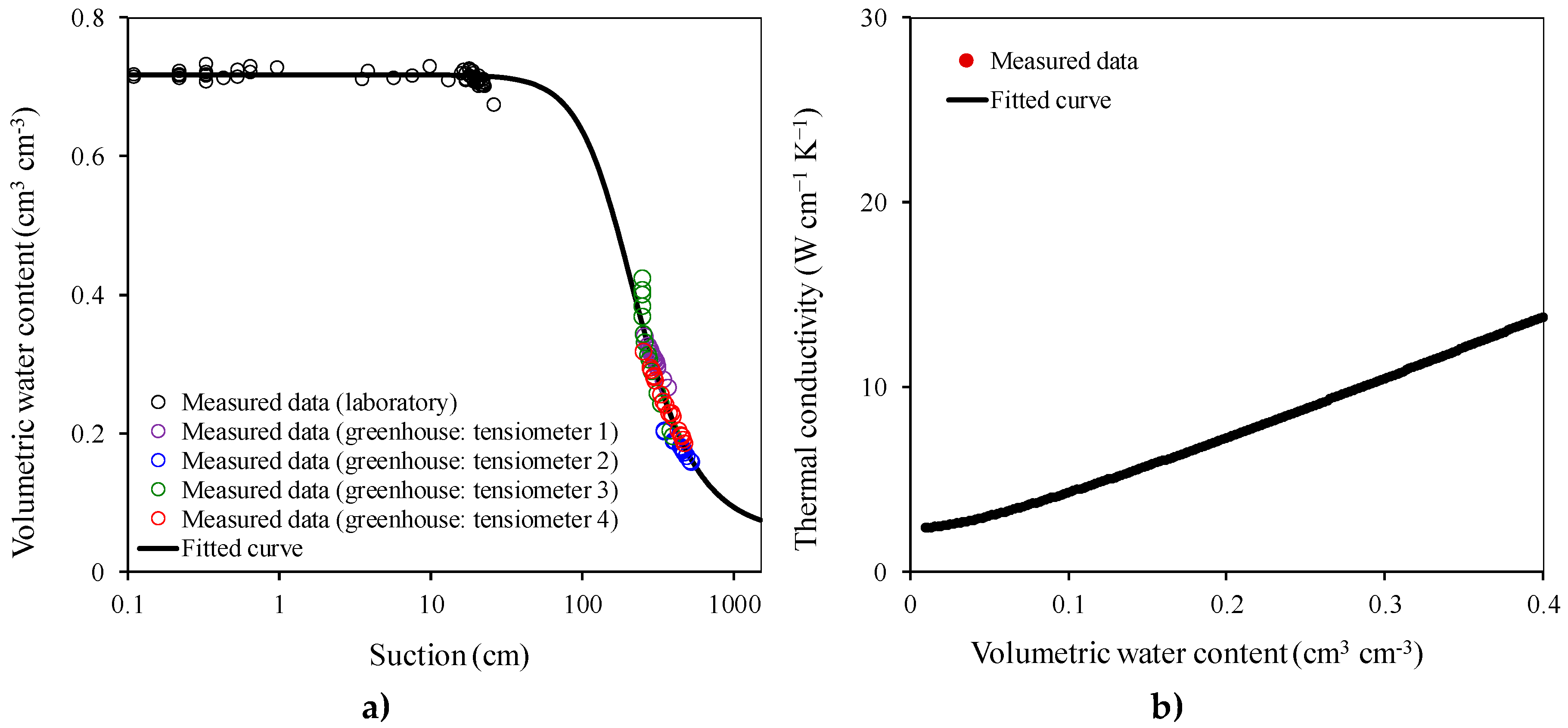
We used 2100F tensiometers and 5TE sensors to directly measure the soil water characteristic curve of the culture substrate in the greenhouse during the cultivation period. Figure 2a shows the result of soil water characteristics curve of the culture substrate during the drainage stage. The black circles in Figure 2a indicate the results that are measured in the laboratory under saturated conditions, and the other color circles (purple, blue, green, and red circles) are the results measured in the greenhouse under unsaturated conditions during the tomato growth period. In the greenhouse, water was drained through the holes in the bottom of the baskets, making it difficult for the culture substrate to achieve saturation. We used a container to fill the culture substrate and inject water to achieve a saturated situation in the laboratory. The black curve was fitted by van Genuchten’s model (Equation (5)) with the parameters α = 0.006 cm−1, n = 2.62, m = 0.62, θ s = 0.72 cm3 cm−3, and θ r = 0.05 cm3 cm−3. This curve illustrates the soil water retention characteristics of the culture substrate. A zero matric potential indicates that the soil is saturated. The culture substrate has a high saturated water content of 0.72 cm3 cm−3, which means that it retains more water than ordinary soil in the saturated situation.
The saturated hydraulic conductivity ( K s ) of culture substrate was determined based on Darcy’s law via the constant-head experiment. The experiment was carried out using glass filter columns (inner diameter = 2.6 cm; length = 30 cm). A Mariotte’s bottle was connected through a silicone tube and a valve to the column to control the hydraulic head. The bottle was placed on an analytical balance (Practum 3102-1S, Sartorius AG, Göttingen, Germany). We converted the measured weight change into flux and calculated K s from the known hydraulic head. The measured saturated hydraulic conductivity of the culture substrate was K s = 57.02 cm day−1.
Furthermore, we used two heat flux transducers to measure the thermal conductivity of the culture substrate. Based on Fourier’s law, the thermal conductivity was obtained from the measured heat flux and the temperature gradient. Figure 2b shows the change of thermal conductivity of the culture substrate with volumetric water content. The fitted curve was fitted by the thermal conductivity equation of Chung and Horton, 1987, λ 0 ( θ ) = b 1 + b 2 θ + b 3 θ 0.5 , with the parameters b 1 = 2.78 W cm−1 K−1, b 2 = 40.34 W cm−1 K−1, and b 3 = −8.15 W cm−1 K−1.

2.4. Processing and Analyzing Data

These soil temperature and volumetric water content data were collected every minute by the data-logger (CR1000) and averaged into hourly data. The air temperature per 5 minutes in the greenhouse was also averaged into hourly data. The outliers were directly removed before averaging. After conversion to the hourly average data, the first 2000 h of data were used as a training set (20 September 2018 to 12 December 2018), and the subsequent 200 h of data were used as a test set (12 December 2018 to 20 December 2018). Finally, we selected an additional 48 h of data (29 December 2018 to 30 December 2018) combined with the weather forecast for prediction analysis. Moreover, the parameters required for the physical models were obtained through various experiments.

3. Physical and Numerical Models

3.1. Physical Models

3.1.1. Newton’s Law of Cooling

In soil heat transport, we used a simple physical model for comparison with data-based or data-driven mathematical models in this study. We assumed a uniform temperature in the soil. Using Newton’s law of cooling [24], the soil temperature can be described by:
d T s d t = k ( T s T a )
where T s (°C) is the soil temperature, T a (°C) is the air temperature in the greenhouse, k [T−1] is a cooling constant, and t [T] is time.
We used the training set to fit the k of each basket with the least square method and validated k by using the test set. The simulated soil temperature value was calculated from the shift terms of Equation (1), T s ( ξ + 1 ) = k ( T s ( ξ ) T a ( ξ ) ) ( t ( ξ + 1 ) t ( ξ ) ) + T s ( ξ ) , where ξ = 1 ,   2 depending on the segmented time. The inputs and outputs of the equation are shown in Table 1.

3.1.2. HYDRUS-1D

HYDRUS-1D has been widely applied to simulate the one-dimensional movement of water and heat in soil [12,25]. It simulates soil heat transport by using the soil heat conduction equation [12], which includes heat convection terms caused by liquid water:
C p T s t = z [ λ ( θ ) T s z ] C w q L T s z C w S T s
where θ (L3 L3) (e.g., m3 m3) is the soil volumetric water content, C w and C p (ML1 T2 K1) (e.g., J m3 K1) are the volumetric heat capacities of water and moist soil, respectively, q L (L T1) (e.g., m s1) is the flux density of liquid water, S (L3 L3 T10 (e.g., m3 m3 s1) is a sink term, z (L) is vertical distance, and λ ( θ ) (ML T3 K1) (e.g., Wm1 K1) is the apparent soil thermal conductivity. λ ( θ ) can be estimated from:
λ ( θ ) = λ 0 ( θ ) + β T C w | q L |
where β T [L] is the thermal dispersivity, and the thermal conductivity ( λ 0 ) can be set in HYDRUS-1D using either the Campbell model [26] or Chung and Horton model [27]. In this study, we used the Chung and Horton model to estimate λ 0 of the culture substrate from the measured data for soil heat flux and temperature in the greenhouse, and the result is shown in Figure 2b.
In HYDRUS-1D, the soil water movement is solved using the Richards’ equation for uniform water flow [12]:
θ t = z [ K ( h z + cos β ) ] S
where h (L) is the matric potential, K (L T1) is the unsaturated hydraulic conductivity, and β is an angle between the flow direction and the vertical axis, where β = 0° for vertical flow. The soil water retention model [28] and soil hydraulic conductivity model [29] are presented as:
θ ( h ) = { θ r + θ s θ r [ 1 + | α h | n ] m h < 0 θ s h 0
K = K s S e L [ 1 ( 1 S e 1 m ) m ] 2
where K s (L T1) is the saturated hydraulic conductivity, S e is the effective saturation, S e = ( θ θ r ) / ( θ s θ r ) , θ s and θ r (L3 L3) are the residual and saturated water content, respectively, and L , α , n , and m are four independent parameters.
As shown in Equations (2) and (4), soil water movement and soil heat transport are described by physical models. We used the HYDRUS-1D model in the direct mode with the measured/empirical parameters, including α , n , m , θ s , θ r , L , K s , Δ z , b 1 , b 2 , b 3 , β , β T , S , C p , C w , q L , and the soil temperature data for upper and lower boundaries (as shown in Table 1), to simulate and predict the soil temperature and volumetric water content.

3.2. Random Forest

In machine learning, the ensemble learning method combined with decision trees comprises the famous random forest model [30]. Breiman, 1996 [31] conducted the bagging method, which is divided into the random selection, classifier training, and majority vote steps, to randomly select subsets by randomizing the training data sets. Breiman, 2001 [30] proposed a random forest model by establishing decision trees that minimized the variance for each subset. The random forest model via the bagging method can effectively improve accuracy and build a mathematical regression model of training data to predict or make decisions without realizing the real physical mechanism. More detailed information on the random forest model can be found in Breiman, 2001 [30].
The use of the random forest model includes two parts: random forest modeling and a simulation or prediction based on the random forest classifier from the modeling. A random forest regression model is an ensemble classifier composed of a set of decision tree classifiers [30]. We applied the bagging method to establish a set of trained classifiers and then classified new data points by taking a vote, which could be weighted on their prediction or decision [32]. By voting and randomly selecting and thus establishing powerful decision trees controlling correlations, the random forest model can thoroughly cover the trained set. The random forest classifier is then verified or calibrated by using the test set.
In this study, we used the scikit-learn package [33] in the Python language to establish the random forest regression model with the training set of 2000 h. There are three adjustable parameters that affect modeling and must be set in advance: the number of decision trees (n_estimators), the maximum depth of each tree (max_depth), and the minimum number of samples required to split an internal node (min_samples_split). We fixed the number of trees to 100 as a compromise between accuracy and efficiency. The maximum depth of trees was set to unlimited, which meant that the nodes would expand until all leaves contained less than min_samples_split samples. The third parameter was set to 2 (min_samples_split = 2), which controlled a subset that was the minimum number of samples for each split.
For simulating and predicting soil temperature, the current air temperature data, the air temperature at the previous time point (1 h earlier), and the soil temperature at the previous time point (1 h earlier) from the training set acted as the input layer and the current soil temperature data was the output layer. For soil volumetric water content, the current air and soil temperature, the air and soil temperature at the previous time point (1 h earlier), the volumetric water content at the previous time point (1 h earlier), and the volumetric water content at the previous two-time points (2 h earlier) acted as the input layer, while the current volumetric water content was the output layer. These inputs and outputs of the random forest model are shown in Table 1. The layers were calculated by using the hidden layer established by the regression tree. Then, the test set was used to verify the random forest classifier. We modeled the prediction method of soil temperature and volumetric water content for tomato growth by the random forest model with the training and test set. Furthermore, this prediction method was used to predict soil temperature and volumetric water content from weather forecast data.

3.3. Inferring Connections of Networks (ICON)

ICON assumes that there are dynamic interactions between units within a complex network. Each unit in the network follows the dynamical law, including the effects of self-dynamics and those from other units [18]:
x ˙ i ( t ) = f ( x i ) + j = 1 j i N K i j ( x i , x j ) ,     i = 1 , , N
where x i ( t ) is the vector of state of unit i at time t , f represents baseline dynamics, K i j is a coupling function between unit i and j , and N is the number of units. Both f and K i j are time series functions, specifically, which can be constituted by orthonormal bases of the individual truncated series [18]. Thus, Equation (7) becomes:
x ˙ i ( t ) = k = 1 M a k Q k ( x i ) + j = 1 j i N k = 1 r l = 1 r b i j k l P k ( x i ) P l ( x j ) ,     i = 1 , , N
where a k and b i j k l are the scalar coefficients, { Q k ( x i ) } k = 1 and { P k ( x i ) } k = 1 constitute orthonormal bases of the respective function spaces containing f and K i j , M is the number of data points in the time series, and r value is the largest order of the Fourier series. By using the orthonormal basis representation of Equation (8), the complex nonlinear topological estimation of each unit i can be converted into a typical linear inverse problem:
min   y ( i ) A ( i ) z ( i )
where y ( i ) is the data vector, A ( i ) is a matrix composed of the orthonormal bases, and z ( i ) is the coefficient vector.
In this study, we established an ICON framework without presumptions on the various impact factors to describe the complex interactions, which may be a nonlinear dynamical relationship consisting of air temperature, soil temperature, volumetric water content, and plants at different temporal scales. Then, the dynamic interactions between units and units were expressed as:
{ x ˙ 1 ( t ) = f ( x 1 ) + K 12 ( x 1 , x 2 ) + K 13 ( x 1 , x 3 ) x ˙ 2 ( t ) = f ( x 2 ) + K 21 ( x 2 , x 1 ) + K 23 ( x 2 , x 3 ) x ˙ 3 ( t ) = f ( x 3 ) + K 31 ( x 3 , x 1 ) + K 32 ( x 3 , x 2 )
We applied the Fourier series to the orthogonal basis of the coupling function of the ICON. Then, Equation (8) is rewritten as:
x ˙ i ( t ) = k = 1 M [ a i k sin ( k x i ) + b i k cos ( k x i ) ] + j = 1 j i N k = 1 r ξ i j k   [ sin ( k x i ) sin ( k x j ) ] + η i j k   [ cos ( k x i ) cos ( k x j ) ] ,     i = 1 , , N
where a i k , b i k , ξ i j k , and η i j k are the coefficients of the Fourier series. In the simulation stage, where N = 3, x 1 , x 2 , and x 3 are the soil temperature, air temperature, and volumetric water content, respectively. In the prediction stage, which is combined with the weather forecast, N = 4, and x 4 is the outdoor air temperature of the weather forecast. A ( i ) and z ( i ) are expressed as:
A ( i ) = [ L 1 ( i ) | | L m ( i ) | G 1 ( i ) | | G m ( i ) | S 1 ( i ) | | S r ( i ) | C 1 ( i ) | | C r ( i ) | ]
z ( i ) = ( z L 1 ( i ) , , z L m ( i ) , z G 1 ( i ) , , z G m ( i ) , z S 1 ( i ) , , z S r ( i ) , z C 1 ( i ) , , z C r ( i ) )
where:
L k ( i ) = [ sin ( k x i ( t 1 ) ) sin ( k x i ( t M ) ) ] ,   G k ( i ) = [ cos ( k x i ( t 1 ) ) cos ( k x i ( t M ) ) ] , S k ( i ) = [ sin ( k x i ( t 1 ) ) sin ( k x 1 ( t 1 ) ) sin ( k x i ( t 1 ) ) sin ( k x N ( t 1 ) ) sin ( k x i ( t 1 ) ) sin ( k x 1 ( t 1 ) ) sin ( k x i ( t M ) ) sin ( k x N ( t M ) ) ] , C k ( i ) = [ cos ( k x i ( t 1 ) ) cos ( k x 1 ( t 1 ) ) cos ( k x i ( t 1 ) ) cos ( k x N ( t 1 ) ) cos ( k x i ( t 1 ) ) cos ( k x 1 ( t 1 ) ) cos ( k x i ( t M ) ) cos ( k x N ( t M ) ) ] .
The training set, where M = 2000, was used to build x i ( t 1 ) to x i ( t M ) and fit the optimum r in our ICON model. The inputs and outputs of the ICON model are shown in Table 1. The test set was used to verify the simulation results from the built ICON model. Because the ICON model was based on the dynamic interactions between factors that affected each other, the simulation for the soil temperature and volumetric water content will be discussed individually in Section 4.3. In the prediction stage, the weather forecast data were added as a unit, and then the ICON model was rebuilt. Finally, we predicted the air temperature, soil temperature, and volumetric water content based on the 1–48 h future weather forecast.

4. Results and Discussion

4.1. Temperature

4.1.1. Temporal Distributions of Air Temperature ( T a ) and Soil Temperature ( T s )

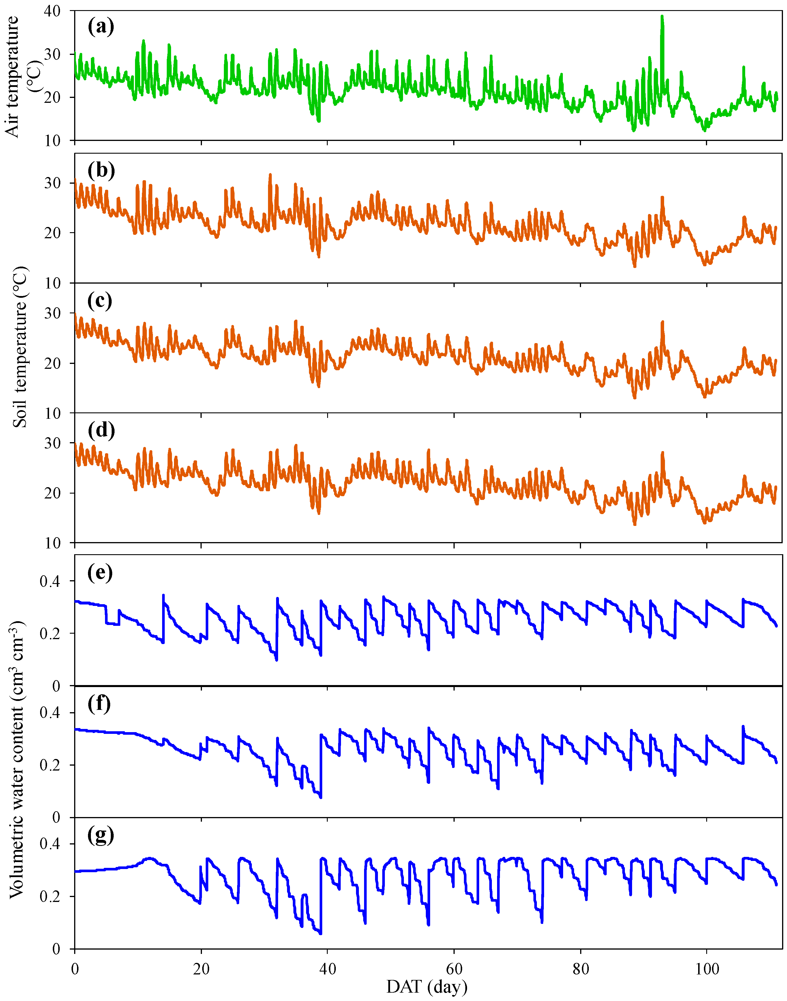
Figure 3a shows the temporal distribution of measured air temperature in the greenhouse during the cultivation period. The observation period of Figure 3a was from September 20, 2018 to January 9, 2019, and the days after transplanting totaled 112. The average air temperature was 25 °C during the cultivation period. The air temperature showed a tendency of daily temperature oscillation. The maximum air temperature observed was 38.8 °C, which occurred at noon on 93rd DAT, and the minimum temperature was 12.1 °C, which occurred at night on 100th DAT. The air temperatures of the greenhouse are easily affected by outdoor temperatures. In this study, these measured air temperatures were used as input data for simulating and predicting soil temperatures and volumetric water contents.
Figure 3b–d shows the temporal distribution of measured soil temperatures of the three culture substrates (basket No. 12, No. 13, and No. 14) in the greenhouse during the cultivation period. Similar trends were observed between these three culture substrates. The soil temperatures were between 13 °C and 31.7 °C, and the average soil temperature was 21.5 °C. The maximum soil temperature of the three culture substrates occurred on the 31st DAT, and the air temperature also reached a relatively high temperature of 30.1 °C. Moreover, the minimum soil temperature occurred on the 89th DAT, and the air temperature was a relatively low temperature of 12.3 °C. The maximum or minimum soil and air temperatures occurred on similar days. This indicates a clear relationship between the soil and the air temperatures [34]. We established the relationship between the air and soil temperature by using Newton’s law of cooling, HYDRUS-1D with measured/empirical parameters, the random forest model with training data, and the ICON model, respectively.

4.1.2. Simulation and Verification of Soil Temperature

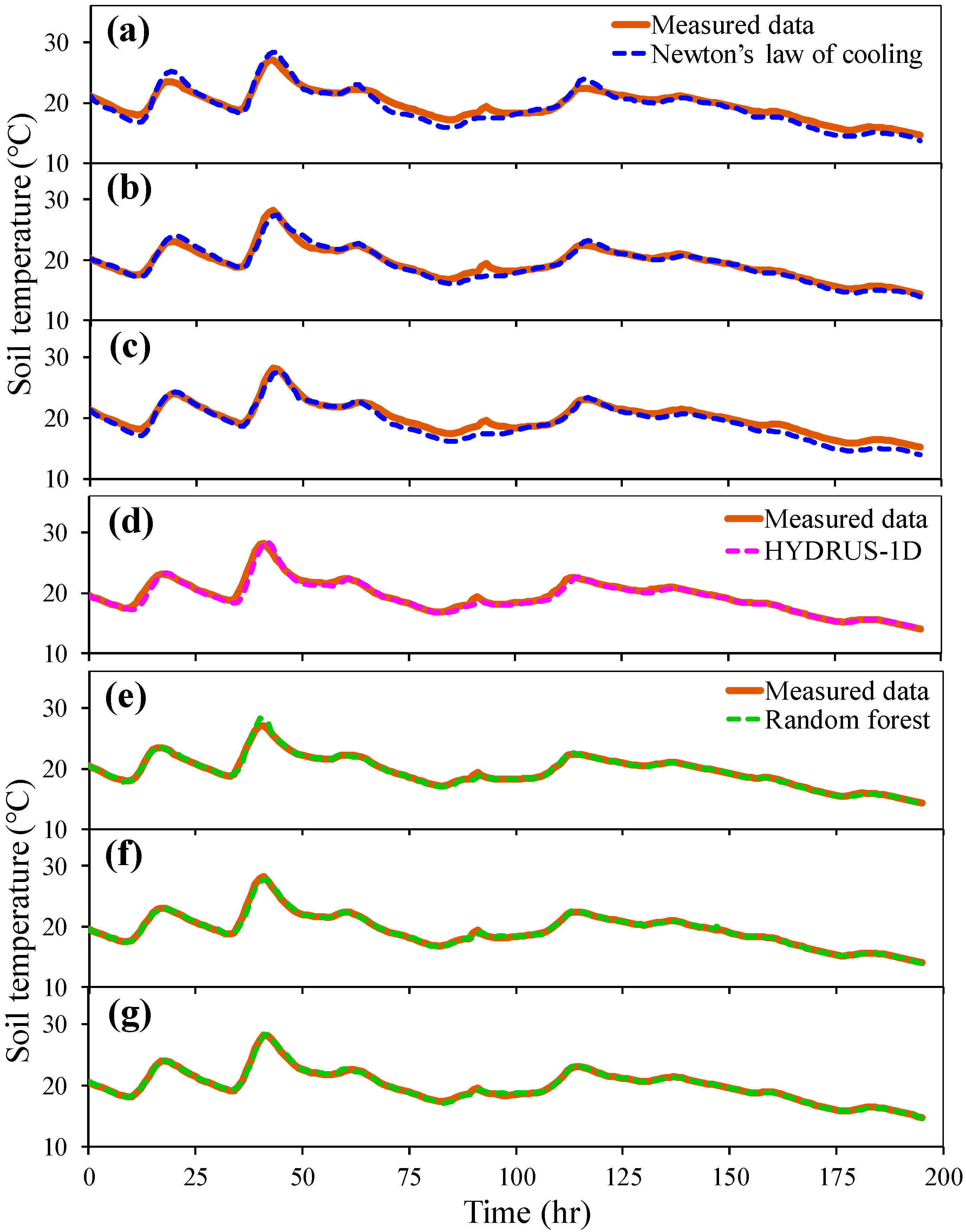
Figure 4a–c shows the soil temperature simulation by Equation (1) with k = −0.306 h−1, k = −0.214 h−1, and k = −0.221 h−1 for baskets No. 12, No. 13, and No. 14, respectively. The air and soil in the greenhouse were regarded as two individuals that transferred heat interactively, and we assumed that the temperature of soil was represented by the central temperature at the soil profile and did not change with depth. In Figure 4a–c, the orange lines are the test set of the measured soil temperature. The values observed in different baskets were slightly different, presumably because of the different volumetric water contents and the spatial distribution of the baskets. Nonetheless, the trends for the soil temperatures between the three baskets were the same. The blue dashed lines were simulated by Newton’s law of cooling (Equation (1)) with k . The simulation results were roughly consistent with the measured values, but there was still a slight difference in that the peaks deviated by approximately 1 h. The peak deviation of 1 h comes from the differentiation of the input data. The advantage of Newton’s law of cooling is that it uses a single parameter to describe the relationship between air temperature and soil temperature; however, it cannot accurately represent the influence of other factors on the heat transfer, such as water content, soil structure, or soil particle arrangement.
We also used HYDRUS-1D and the measured/empirical parameters to simulate soil temperatures and compare them with the measured data. Since measured data for soil temperature in the upper and lower boundaries were only available in basket No. 13, it will be the only basket discussed for the simulation by HYDRUS-1D in this section. Figure 4d shows the soil temperature simulation by HYDRUS-1D with the measured/empirical parameters. The magenta dashed line was simulated by HYDRUS-1D. The result of the simulation was more accurate than that of Newton’s law of cooling. Specifically, in the interval of 80 h to 100 h, the deviation was smaller than Newton’s law of cooling. When all the required parameters of the HYDRUS-1D model can be provided, the physical model should become efficient enough to predict soil temperature and water content without having to collect long-term monitoring data. Moreover, the setup of the HYDRUS-1D model can also be easily transferred or extrapolated to represent other farms with different environmental conditions. In fact, without considering the effect of crops, the prediction from HYDRUS-1D was already close to the observation initially. However, the HYDRUS-1D simulation results still had a peak deviation of 1 h. Using HYDRUS-1D requires many measured parameters that must be prepared in advance, which means that we would need further experimental analysis and additional instruments or measurements to obtain parameters. Moreover, the complicated interaction between crops and the soil temperature and water content is not fully considered in most of the physical models.
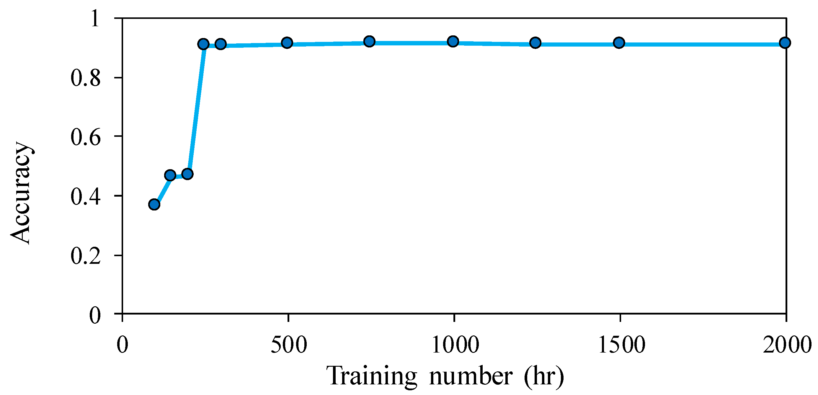
For the random forest model, we first tested the relationship between the number of trainings and simulation accuracy, as shown in Figure 5. The accuracy is calculated by dividing the correct number of the random forest model into the total number of trainings. The accuracy exceeded 0.9 with more than 250 training numbers in our case. More accurate simulations can be achieved when the training numbers cover all possible scenarios (e.g., irrigation events), although this accuracy depends on the training numbers themselves [13]. To cover all the scenarios during the cultivation period and compare them with the other models, we used the same 2000-h training set to establish the random forest regression model. Figure 4e–g shows the simulation results (green dashed lines) of soil temperature by the random forest model. The result is a useful description for the measured data (orange lines). Compared with Figure 4b,d, the simulation result (Figure 4f) of the random forest model is more accurate, and the peak deviation is negligible. The random forest model can automatically learn the relationship between the air and soil temperatures through these training data, including the time lag; thus, the simulated soil temperature can be in close accordance with the measured value, which is different from the aforementioned physical models. However, the weakness of the machine learning technique is that it is impossible to simulate or predict the soil temperature directly from the air temperature without training data. A large amount of training data is required to support the model’s simulations or predictions [13].
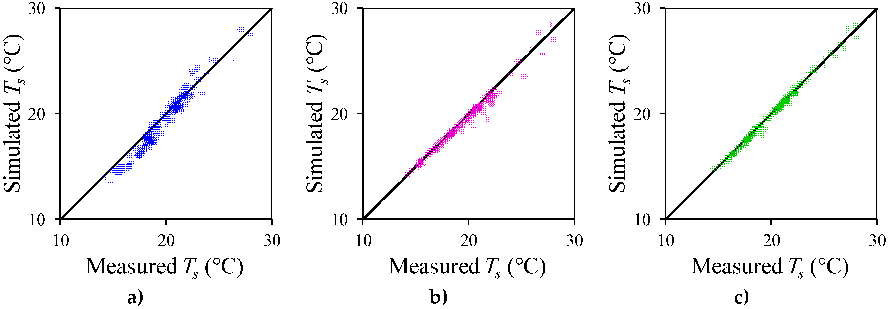
Figure 6 shows a comparison of the measured and the simulated soil temperature as determined by Newton’s law of cooling, HYDRUS-1D, and the random forest model. The circles in Figure 6c overlap on the straight line better than Figure 6a,b, to verify that the random forest model simulations are more accurate than those determined by Newton’s law of cooling and HYDRUS-1D. The root mean square error (RMSE) and Nash-Sutcliffe model efficiency coefficient (NSE) between the measured soil temperature and the simulated soil temperature was also calculated to compare the simulation performances of these models. The RMSEs of soil temperatures for Newton’s law of cooling, HYDRUS-1D, and the random forest model were 0.763 ± 0.133 °C, 0.469 °C, and 0.201 ± 0.020 °C, respectively. The NSEs of soil temperatures as per Newton’s law of cooling, HYDRUS-1D, and the random forest model were 0.905 ± 0.033 °C, 0.970 °C, and 0.994 ± 0.001 °C, respectively. The results are shown in Table 2.

4.2. Volumetric Water Content

4.2.1. Volumetric Water Content During the Cultivation Period

Figure 3e–g shows the temporal distribution of measured soil volumetric water contents in three baskets during the cultivation period, which was measured from September 20, 2018 to January 9, 2019 (DAT = 112 days). These three baskets did not undergo water-saving treatments but were manually irrigated with the same frequency. In Figure 3e, the measured data was abnormal during the DAT period of 6 to 7 due to a problem with the moisture sensor in basket No. 12, and the sensor was immediately rechecked and relocated.

4.2.2. Simulation and Verification of Volumetric Water Content

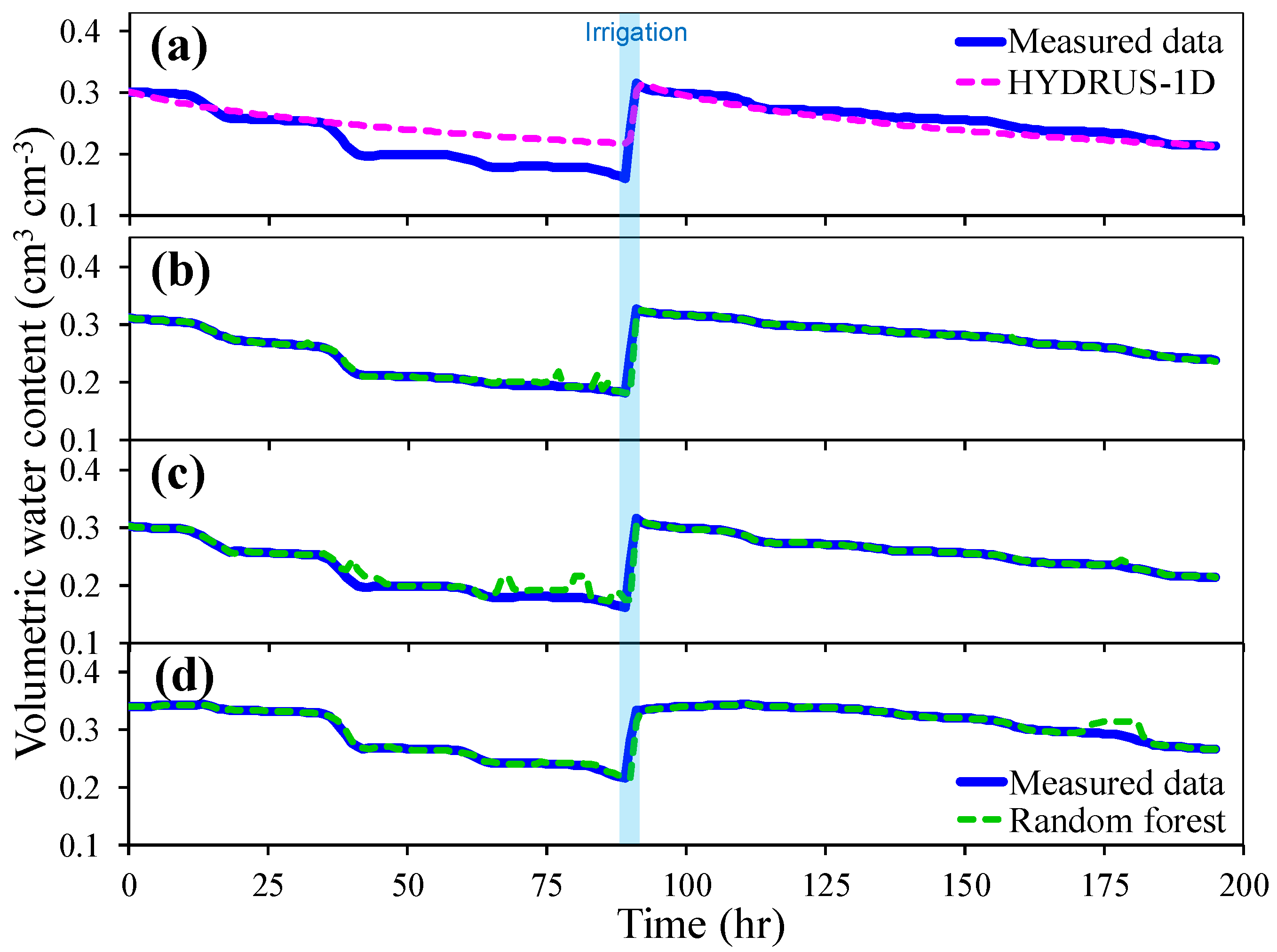
Figure 7a shows the simulation result of soil volumetric water content by HYDRUS-1D with the measured/empirical parameters in basket No. 13. The blue line was the test set of the measured volumetric water content, and the magenta dashed line was simulated by HYDRUS-1D. At the 89th hour of the irrigation event, the sudden increase in the simulated water content was due to the boundary conditions containing the information about the changes in matric potential. Overall, the simulation result after 89 h was closer to the measured values than before 89 h, and the measured volumetric water contents before 89 h were much lower than the simulated values. Due to the effect of high temperature from the 38th to the 41st hour (air temperature = 28.5–30.8 °C, soil temperature = 25.2–28.3 °C), the accelerated evapotranspiration caused the soil water content to decrease rapidly, which deviated from the ideal simulation by the model, and the water content did not increase until the irrigation event at the 89th hour. Moreover, the measured volumetric water contents (blue line) had a significant one-step declining trend with time. Due to the rotation between day and night, plant evapotranspiration was more pronounced during the day, causing a steeper slope; at night, photosynthesis stopped, thus, water consumption decreased and the decline in the volumetric water content curve was gentler. This situation cannot be simulated by HYDRUS-1D. As a result, any influencing factors will reflect the observed soil temperature and soil water content, which increases the difficulty of the model’s ability to simulate soil temperature and soil water content.
Figure 7b–d shows the simulation results of soil volumetric water content by the random forest model in the three baskets. The blue lines are the test set of the measured volumetric water content. The green dashed lines were simulated by the random forest model. The simulation accuracy of the random forest model was higher than that of HYDRUS-1D. Specifically, the increase in volumetric water content caused by irrigation events during the training stage was included in the training set. These events were learned by the random forest model with the input features, especially for the changes in the volumetric water content of the previous time point (1 h earlier) and the volumetric water content at the previous two-time points (2 h earlier). Therefore, the simulated values (green dashed lines) show a sudden increase in the figure (e.g., Figure 7b 70–89 h; 7c 35–89 h; and 7d 170–180 h). This means that the random forest model has the potential to suggest irrigation needs when the volumetric water content continues to decrease.
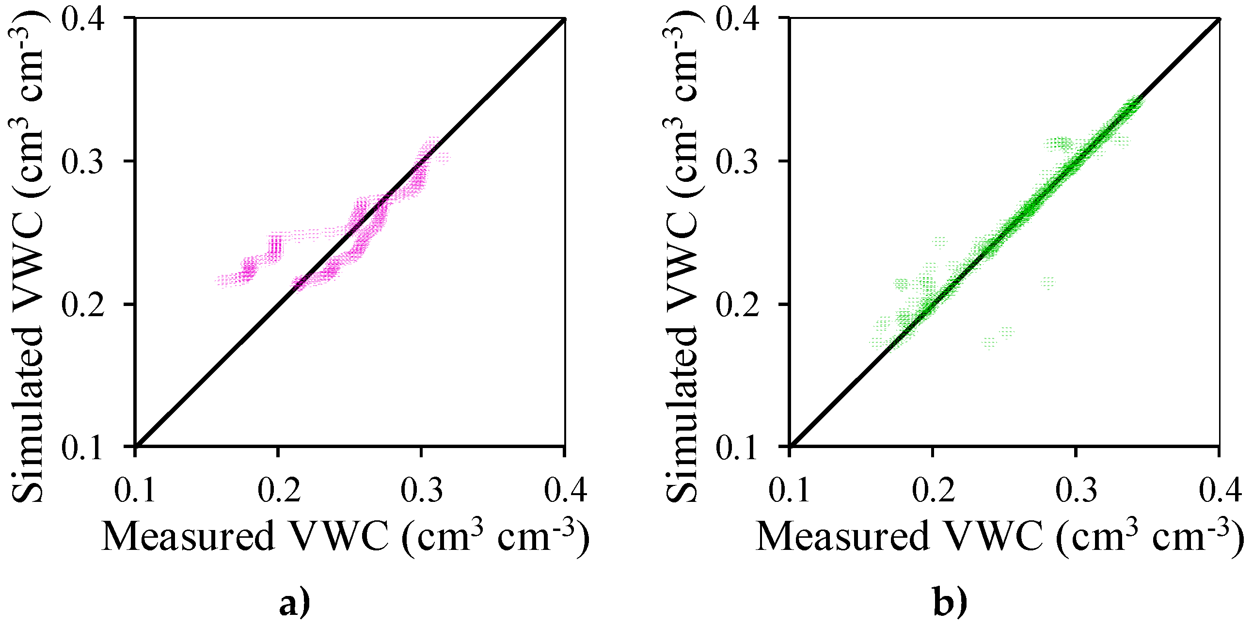
Figure 8 shows the comparison of the measured and simulated soil volumetric water content by HYDRUS-1D and the random forest model. Compared with Figure 8a, the green circles of the random forest model in Figure 8b overlap better on the straight line. Moreover, Table 2 shows that the RMSEs of soil volumetric water content for HYDRUS-1D and the random forest model are 0.024 cm3 cm−3 and 0.008 ± 0.001 cm3 cm−3, along with the NSEs of 0.626 cm3 cm−3 and 0.961 ± 0.014 cm3 cm−3, respectively. The simulation performance of the random forest model on the soil volumetric water content is more accurate than that of HYDRUS-1D.

4.3. ICON Simulation Based on Interactions Between Air Temperature, Soil Temperature, and Volumetric Water Content

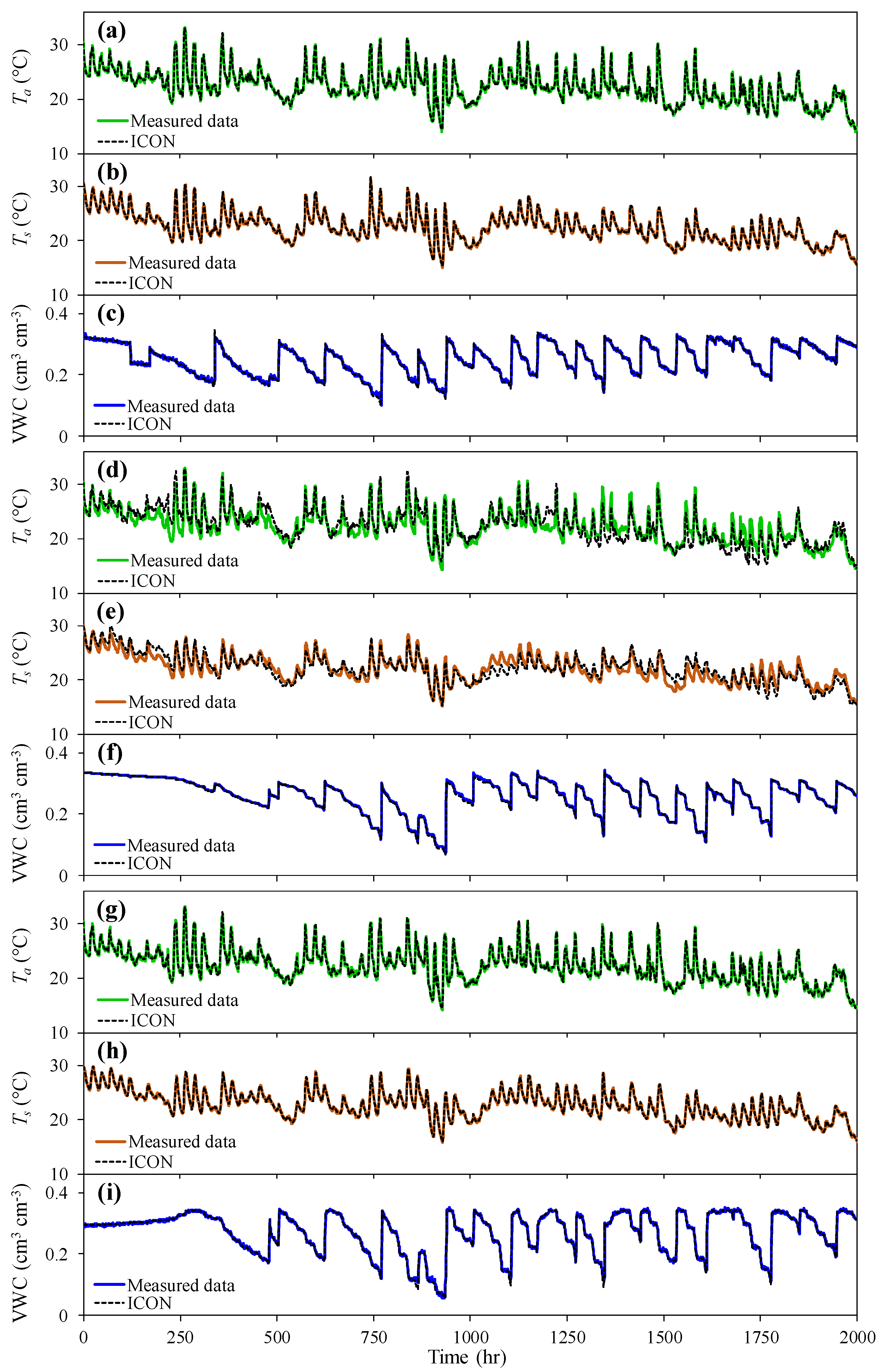
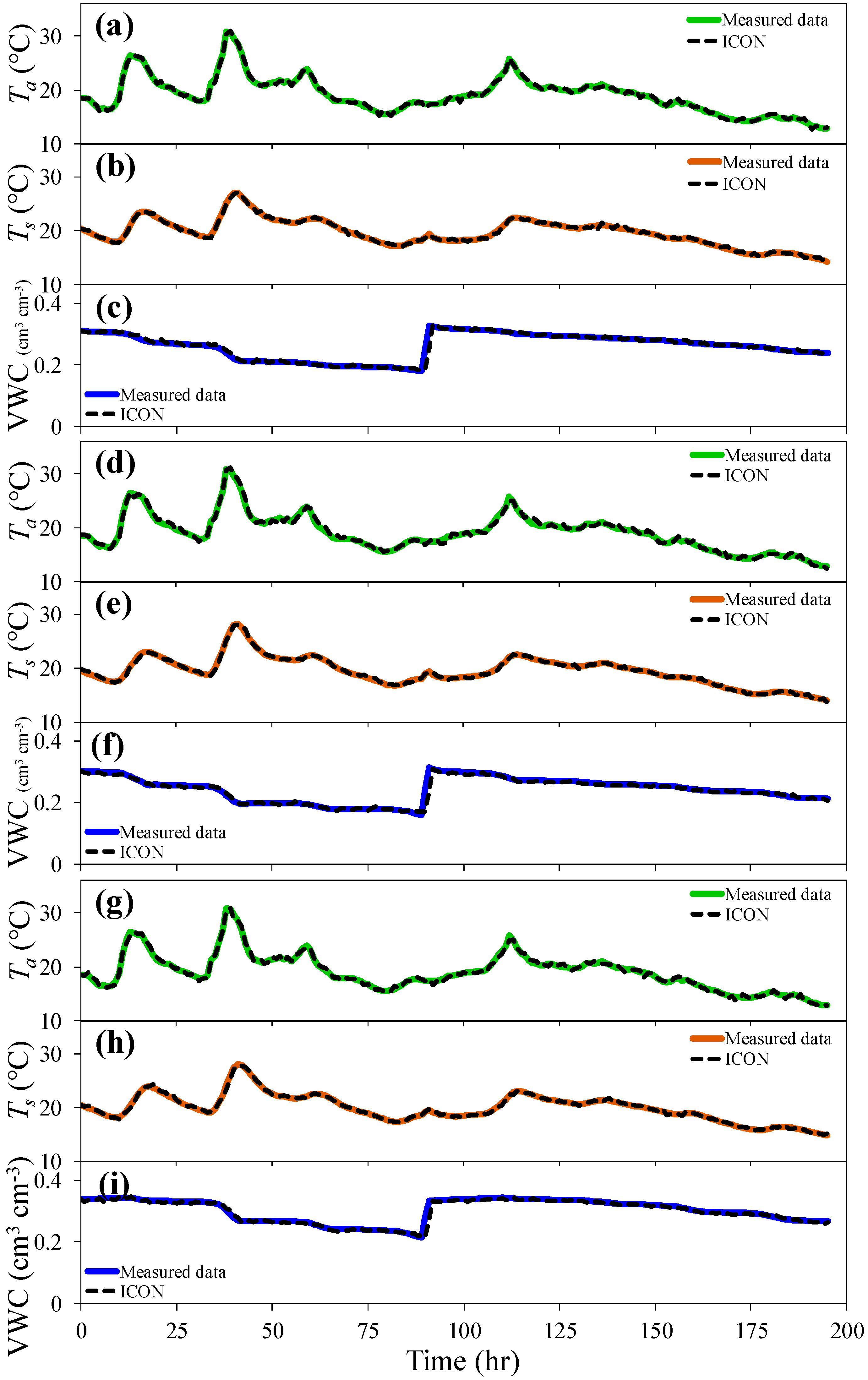
Figure 9 shows the establishment of the ICON model for baskets No. 12, No. 13, and No. 14 via the interactions between the soil temperature, air temperature, and volumetric water content, which affect each other dynamically. The green, orange, and blue lines are the measured data of the training set. The fitted curves (black dashed lines) with the largest orders of Fourier series were as follows: r = 333, 285, and 318 for the soil temperature, r = 333, 282, and 325 for the air temperature, and r = 37, 48, and 31 for the volumetric water contents in baskets No. 12, No. 13, and No. 14, respectively. Larger r values more accurately depict real dynamic interactions [18]. Depending on the complexity of the patterns in the training set, the r values of air temperature and soil temperature were much larger than that of the volumetric water content.
Figure 10a–i shows that the simulation results (black dashed lines) of the ICON model, which was established by the aforementioned fitting, compared with the test set (green, orange, and blue lines) of the measured soil temperature, air temperature, and volumetric water content. Among these three factors, the volumetric water content has the most accurate simulation result, and the soil temperature and air temperature are also in accordance. Although the simulation results have some small fluctuations, especially in the simulation result of air temperature, these small fluctuations fortunately do not affect the simulation trend.
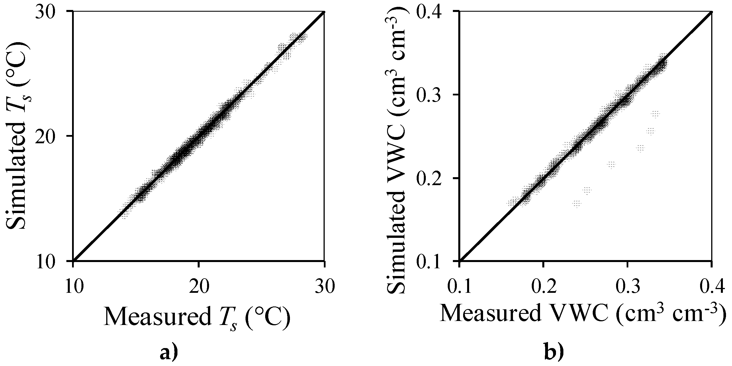
Figure 11 shows the comparison of the measured and the simulated values by the ICON model for soil temperature and volumetric water content. The RMSE of soil temperature for the ICON model is 0.206 ± 0.006 °C, and the NSE is 0.994 ± 0.001 °C (as shown in Table 2). The simulation performance of the ICON model for soil temperature is more accurate than that for Newton’s law of cooling (RMSE = 0.763 ± 0.133 °C, NSE = 0.905 ± 0.033 °C) and HYDRUS-1D (RMSE = 0.469 °C, NSE = 0.970 °C); similar to the random forest model (RMSE = 0.201 ± 0.020 °C, NSE = 0.994 ± 0.001 °C). The RMSE of the volumetric water content for the ICON model is 0.008 ± 0.001 cm3 cm−3, and the NSE is 0.962 ± 0.004 cm3 cm−3. The simulation performance of the ICON model for volumetric water content is more accurate than HYDRUS-1D (RMSE = 0.024 cm3 cm−3, NSE = 0.626 cm3 cm−3) and similar to the random forest model (RMSE = 0.008 ± 0.001 cm3 cm−3, NSE = 0.961 ± 0.014 cm3 cm−3).
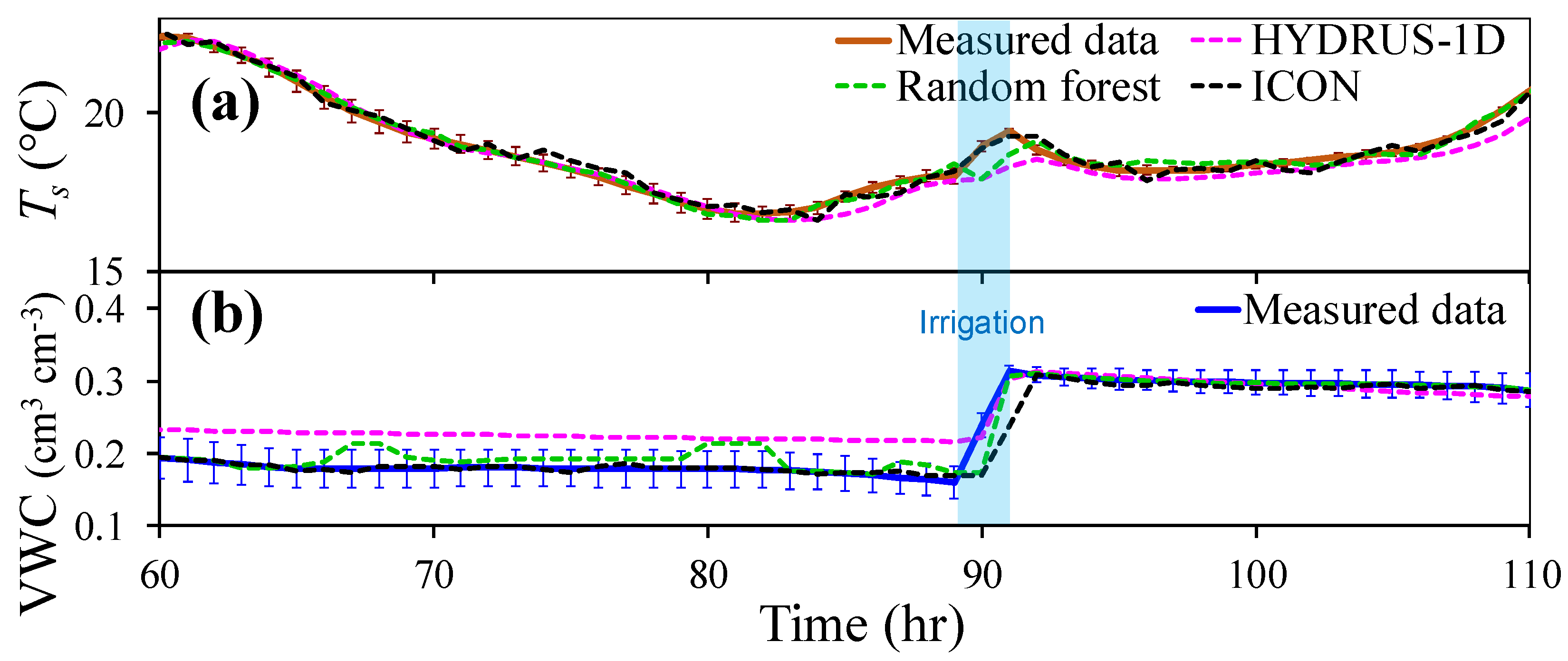
Figure 12 shows the simulation performance of the HYDRUS-1D, random forest model, and ICON model on the measured data with error bars, which represent the standard deviation of the measured data. There was an irrigation event at the 89th hour, as represented in the figure via blue highlights. The simulation results of the random forest model and ICON model for the soil temperature were consistent with the measured values (as shown in Figure 12a). However, during the irrigation event, only the ICON model was observed to respond to the changes in soil temperature that were caused by irrigation. In Figure 12b, both the random forest model and ICON model showed good simulation performance for volumetric water content and were consistent with the measured values. Contrastingly, the prediction of VWC from HYDRUS-1D before the 90th hour was higher than the measured data since HYDRUS-1D was not able to simulate the strong evapotranspiration due to high air temperatures.

4.4. Prediction of Soil Temperature and Volumetric Water Content from the Air Temperature of the Weather Forecast

In this study, we proposed a framework to predict the soil temperature and volumetric water content in a non-temperature-controlled greenhouse via applying HYDRUS-1D, the random forest model, and the ICON model with the weather forecast data. The combined forecast data were used in these prediction models to obtain the changes in soil temperature and volumetric water content over time. The source of weather forecast data (from the Central Weather Bureau, Taipei, Taiwan) is a rolling forecast of hourly outdoor air temperature for the future 48 h, thus, the prediction stage was limited to 1–48 h.
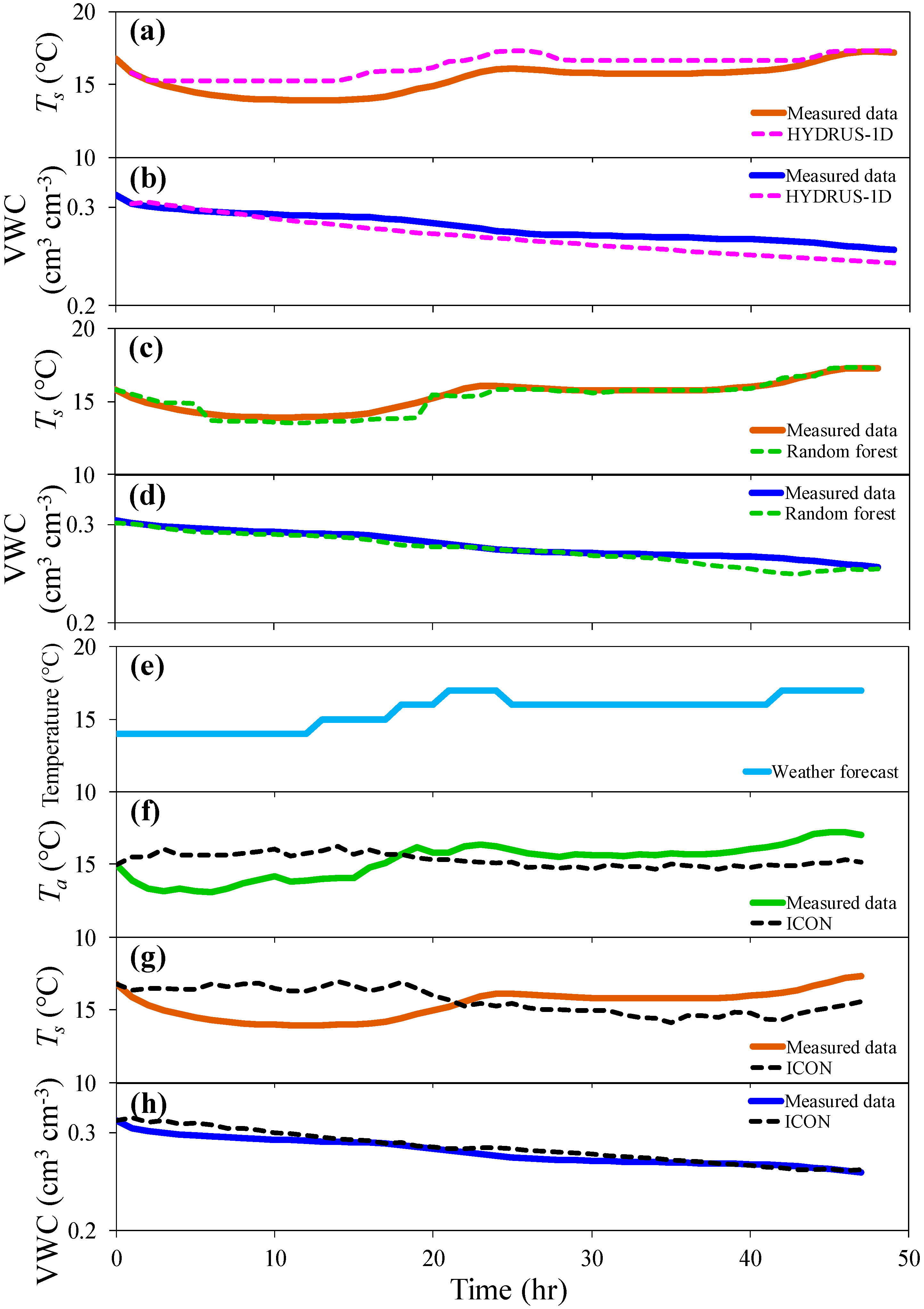
Since the physical equations in HYDRUS-1D were not related to the forecasted outdoor air temperature, we performed a linear regression on 2667 forecasted outdoor air temperatures to establish a conversion equation, T a c o n v e r t = 0.91 T f o r e c a s t + 1.20 (R2 = 0.80), for the indoor air temperature. In addition, the soil temperatures of the upper and lower boundaries required for the model were converted by the linear regression equations, T s u p p e r = 0.83 T a c o n v e r t + 3.18 (R2 = 0.86) and T s l o w e r = 0.75 T a c o n v e r t + 5.19 (R2 = 0.84), with the aforementioned converted indoor air temperature from the soil temperature data. Table 3 lists the inputs and outputs of the conversion. Figure 13a,b shows the prediction results (magenta dashed lines) from the outdoor air temperature data of the weather forecast by HYDRUS-1D with the measured parameters in basket No. 13. The green, orange, and blue lines are the measured data of 48 h. Overall, the prediction results overestimated the soil temperature and underestimated the volumetric water content, but the predictions were generally in accordance with actual trends. The results deviated from the measured values because of restrictions on the model parameters. The RMSEs of the predicted soil temperature and volumetric water content were 1.006 °C and 0.011 cm3 cm−3, respectively, and the NSEs were −0.020 °C and 0.342 cm3 cm−3. The results are shown in Table 4.
For machine learning, during the prediction stage, we directly applied the random forest model to train the indoor air temperature with the forecasted outdoor air temperature. The 24-h time, forecasted outdoor air temperature, and ultraviolet index (UVI) were used as the input layer, and the indoor air temperature data was the output layer (as shown in Table 3). After the training processes, we established a conversion relationship between the weather forecast data and indoor air temperature. When the converted indoor air temperature, T a c o n v e r t , was available, we applied the established random forest model to predict the soil temperature and volumetric water content. Figure 13c,d shows the prediction results (green dashed lines) from the random forest model via training data with the converted indoor air temperature from the forecasted outdoor air temperature in basket No. 13. The prediction results are in accordance with the actual measurement data, and the prediction performance of the random forest model is more accurate than HYDRUS-1D. The RMSEs of soil temperature and volumetric water content predicted by the random forest model were 0.333 °C and 0.006 cm3 cm−3, respectively, and the NSEs were 0.889 °C and 0.795 cm3 cm−3. The results are shown in Table 4.
Finally, we collected the outdoor air temperatures of weather forecasts as an influencing factor and attached them to the ICON model. The ICON model was re-established for tomato planting with the training set via the interactions between four factors, which were soil temperature, indoor air temperature, volumetric water content, and forecasted outdoor air temperature; these factors affected each other dynamically. The largest orders of Fourier series were fitted as follows: r = 250 for the soil temperature, r = 250 for the air temperature, and r = 49 for the volumetric water content. Figure 13e–h shows the prediction results (black dashed lines) from the forecasted outdoor air temperature of as an input factor by the re-established ICON model in basket No. 13. The RMSEs of the predicted soil temperature and volumetric water content were 1.701 °C and 0.006 cm3 cm−3, respectively, and the NSEs were −2.813 °C and 0.850 cm3 cm−3 (as shown in Table 4). The prediction result of the volumetric water content was consistent with the actual measurement data and showed an accurate prediction result. Unfortunately, the partial predictions of soil temperature were inferior to the physical models and random forest model. Regardless, the advantage of the ICON model is that it can extract the dynamic interactions of a large complex system with multiple factors that affect each other dynamically. The reason for the somewhat inaccurate prediction results for soil temperature may be because we used only four factors for the short-term (48 h) prediction, which may have limited the performance of this model.

5. Conclusions

We proposed a novel framework that applied physical models, machine learning methods, and dynamic topology to simulate and predict soil temperature and volumetric water content in a greenhouse in combination with weather forecast data. We used Newton’s law of cooling, HYDRUS-1D, the random forest model, and the ICON model, to simulate and verify the measured soil temperature. HYDRUS-1D, the random forest model, and the ICON model were used to simulate and verify the measured volumetric water content. Moreover, the simulation performances of these models were compared with RMSE. The random forest model was more accurate than the other methods with limited information provided from the greenhouse experiments; this approach also has the potential to suggest irrigation regimes. Additionally, the random forest model and ICON model can use historical data to effectively simulate soil temperature and volumetric water content without physical parameters.
Our study demonstrated the capability of the proposed framework with HYDRUS-1D, the random forest model, and the ICON model to predict soil temperature and volumetric water content based on a future weather forecast of 1–48 h. With limited information, predictions on soil temperature and volumetric water content by the random forest model were more accurate than the other models. Using the three models from our proposed framework should help farmers in choosing a suitable model for their agricultural practices.
Our proposed models can assess the water requirements for agricultural practices and develop water content and temperature alarms for greenhouse management. Moreover, our approach can collect soil and water information of the best practices determined by experienced farmers. By setting the collected data as a training set, our prediction framework can not only learn best management practices from experienced farmers, but it can also provide intelligent information for smart greenhouse management.

Author Contributions

Conceptualization, Y.-Z.T. and S.-Y.H.; Data curation, Y.-Z.T., K.-S.H., and S.-Y.H.; Formal analysis, Y.-Z.T. and K.-S.H.; Funding acquisition, H.-L.Y., K.-T.H., M.-C.H., and S.-Y.H.; Investigation, Y.-Z.T., K.-S.H., H.-Y.W., and S.-I.L.; Methodology, Y.-Z.T., K.-S.H., and S.-Y.H.; Project administration, S.-Y.H.; Resources, H.-Y.W., S.-I.L., K.-T.H., M.-C.H., and S.-Y.H.; Software, K.-S.H.; Supervision, H.-L.Y. and S.-Y.H.; Validation, Y.-Z.T. and S.-Y.H.; Visualization, Y.-Z.T.; Writing—original draft, Y.-Z.T.; Writing—review and editing, Y.-Z.T. and S.-Y.H. All authors have read and agreed to the published version of the manuscript.

Funding

This research was funded by the National Taiwan University (NTU-CC-107L892607) and Ministry of Science and Technology, Taiwan (106-2628-M-002-009-MY3).

Acknowledgments

The authors would like to thank Yu-Pin Lin and Hsiao-Feng Lo from National Taiwan University for the experimental design and thoughtful discussions. This research was funded by National Taiwan University, R.O.C. (Grant No., NTU-CC-107L892607) and the Ministry of Science and Technology, Taiwan, R.O.C. (MOST; Grant No., 106-2628-M-002-009-MY3). Additionally, the authors thank the editors and anonymous referees for their thoughtful comments and suggestions. We gratefully acknowledge the contribution of Yu-Che Lin, a student of National Taiwan University, for assisting in planting tomatoes. The data presented in this study are available through the corresponding author (Shao-Yiu Hsu) upon request ([email protected]).

Conflicts of Interest

The authors declare no conflict of interest.

References

  1. Shannon, H.D.; Motha, R.P. Managing weather and climate risks to agriculture in North America, Central America and the Caribbean. Weather Clim. Extrem. 2015, 10, 50–56. [Google Scholar] [CrossRef] [Green Version]
  2. Gebbers, R.; Adamchuk, V.I. Precision agriculture and food security. Science 2010, 327, 828–831. [Google Scholar] [CrossRef] [PubMed]
  3. Zhang, N.Q.; Wang, M.H.; Wang, N. Precision agriculture—A worldwide overview. Comput. Electron. Agric. 2002, 36, 113–132. [Google Scholar] [CrossRef]
  4. Duarte-Galvan, C.; Torres-Pacheco, I.; Guevara-Gonzalez, R.G.; Romero-Troncoso, R.J.; Contreras-Medina, L.M.; Rios-Alcaraz, M.A.; Mian-Amaraz, J.R. Review. Advantages and disadvantages of control theories applied in greenhouse climate control systems. Span. J. Agric. Res. 2012, 10, 926–938. [Google Scholar] [CrossRef] [Green Version]
  5. Ehret, D.L.; Lau, A.; Bittman, S.; Lin, W.; Shelford, T. Automated monitoring of greenhouse crops. Agronomie 2001, 21, 403–414. [Google Scholar] [CrossRef]
  6. Hodge, A.; Berta, G.; Doussan, C.; Merchan, F.; Crespi, M. Plant root growth, architecture and function. Plant. Soil 2009, 321, 153–187. [Google Scholar] [CrossRef]
  7. Al-Kayssi, A.W.; Al-Karaghouli, A.A.; Hasson, A.M.; Beker, S.A. Influence of soil moisture content on soil temperature and heat storage under greenhouse conditions. J. Agric. Eng. Res. 1990, 45, 241–252. [Google Scholar] [CrossRef]
  8. Hu, H.; Xu, L.; Wei, R.; Zhu, B. Multi-objective control optimization for greenhouse environment using evolutionary algorithms. Sensors 2011, 11, 5792–5807. [Google Scholar] [CrossRef] [Green Version]
  9. Philip, J.R. Evaporation, and Moisture and Heat Fields in the Soil. J. Meteorol. 1957, 14, 354–366. [Google Scholar] [CrossRef] [Green Version]
  10. Nassar, I.N.; Horton, R. Simultaneous transfer of heat, water, and solute in porous media: I. Theoretical development. Soil Sci. Soc. Am. J. 1992, 56, 1350–1356. [Google Scholar] [CrossRef]
  11. Saito, H.; Šimůnek, J.; Mohanty, B. Numerical analyses of coupled water, vapor and heat transport in the vadose zone. Vadose Zone J. 2006, 5, 784–800. [Google Scholar] [CrossRef] [Green Version]
  12. Šimůnek, J.; Šejna, M.; Saito, H.; Sakai, M.; van Genuchten, M.T. The HYDRUS-1D Software Package for Simulating the One-Dimensional Movement of Water, Heat, and Multiple Solutes in Variably-Saturated Media; University of California Riverside: Riverside, CA, USA, 2009; p. 296. [Google Scholar]
  13. Mohri, M.; Rostamizadeh, A.; Talwalkar, A. Foundations of Machine Learning; The MIT Press: Cambridge, MA, USA, 2012; p. 480. [Google Scholar]
  14. Alzubi, J.; Nayyar, A.; Kumar, A. Machine Learning from Theory to Algorithms: An Overview. J. Phys. Conf. Series 2018, 1142. [Google Scholar] [CrossRef]
  15. Ahmad, S.; Kalra, A.; Stephen, H. Estimating soil moisture using remote sensing data: A machine learning approach. Adv. Water Resour 2010, 33, 69–80. [Google Scholar] [CrossRef]
  16. Oroza, C.A.; Bales, R.C.; Stacy, E.M.; Zheng, Z.; Glaser, S.D. Long-Term Variability of Soil Moisture in the Southern Sierra: Measurement and Prediction. Vadose Zone J. 2018, 17. [Google Scholar] [CrossRef]
  17. Karandish, F.; Šimůnek, J. A comparison of numerical and machine-learning modeling of soil water content with limited input data. J. Hydrol. 2016, 543, 892–909. [Google Scholar] [CrossRef] [Green Version]
  18. Wang, S.; Herzog, E.D.; Kiss, I.Z.; Schwartz, W.J.; Bloch, G.; Sebek, M.; Granados-Fuentes, D.; Wang, L.; Li, J.S. Inferring dynamic topology for decoding spatiotemporal structures in complex heterogeneous networks. Proc. Natl. Acad. Sci. USA 2018, 115, 9300–9305. [Google Scholar] [CrossRef] [Green Version]
  19. Shamshiri, R.R.; Jones, J.W.; Thorp, K.R.; Ahmad, D.; Man, H.C.; Taheri, S. Review of optimum temperature, humidity, and vapour pressure deficit for microclimate evaluation and control in greenhouse cultivation of tomato: A review. Int. Agrophys. 2018, 32, 287–302. [Google Scholar] [CrossRef]
  20. Moreno, M.M.; Moreno, A. Effect of different biodegradable and polyethylene mulches on soil properties and production in a tomato crop. Sci. Hortic. Amst. 2008, 116, 256–263. [Google Scholar] [CrossRef]
  21. Li, Y.; Xue, X.; Guo, W.; Wang, L.; Duan, M.; Chen, H.; Chen, F. Soil moisture and nitrate-nitrogen dynamics and economic yield in the greenhouse cultivation of tomato and cucumber under negative pressure irrigation in the North China Plain. Sci. Rep. 2019, 9, 4439. [Google Scholar] [CrossRef]
  22. Chen, R.Q.; Kang, S.Z.; Hao, X.M.; Li, F.S.; Du, T.S.; Qiu, R.J.; Chen, J.L. Variations in tomato yield and quality in relation to soil properties and evapotranspiration under greenhouse condition. Sci. Hortic. Amst. 2015, 197, 318–328. [Google Scholar] [CrossRef]
  23. Sun Gro Horticulture Distribution Inc. Safety Data Sheet: Sunshine® Professional Peat Moss and Peat-Based Mixes. 2015. Available online: http://www.sungro.com/professional-product/sunshine-5-natural-organic (accessed on 28 August 2018).
  24. Besson, U. The History of the Cooling Law: When the Search for Simplicity can be an Obstacle. Sci. Educ. 2010, 21, 1085–1110. [Google Scholar] [CrossRef]
  25. Šimůnek, J.; van Genuchten, M.T.; Šejna, M. Recent developments and applications of the HYDRUS computer software packages. Vadose Zone J. 2016, 15, 1–25. [Google Scholar] [CrossRef] [Green Version]
  26. Campbell, G.S. Soil Physics With BASIC: Transport. Models for Soil-Plant. Systems; Elsevier: Amsterdam, The Netherlands, 1985; p. 150. [Google Scholar]
  27. Chung, S.O.; Horton, R. Soil Heat and Water-Flow with a Partial Surface Mulch. Water Resour. Res. 1987, 23, 2175–2186. [Google Scholar] [CrossRef] [Green Version]
  28. van Genuchten, M.T. A closed-form equation for predicting the hydraulic conductivity of unsaturated soils. Soil Sci. Soc. Am. J. 1980, 44, 892–898. [Google Scholar] [CrossRef] [Green Version]
  29. Mualem, Y. A new model for predicting the hydraulic conductivity of unsaturated porous media. Water Resour Res. 1976, 12, 513–522. [Google Scholar] [CrossRef] [Green Version]
  30. Breiman, L. Random forests. Mach. Learn. 2001, 45, 5–32. [Google Scholar] [CrossRef] [Green Version]
  31. Breiman, L. Bagging predictors. Mach. Learn. 1996, 24, 123–140. [Google Scholar] [CrossRef] [Green Version]
  32. Dietterich, T.G. Ensemble Methods in Machine Learning. In Multiple Classifier Systems, MCS 2000; Kittler, J., Roli, F., Eds.; Springer: Berlin/Heidelberg, Germany; Cagliari, Italy, 2000; pp. 1–15. [Google Scholar]
  33. Pedregosa, F.; Varoquaux, G.; Gramfort, A.; Michel, V.; Thirion, B.; Grisel, O.; Blondel, M.; Prettenhofer, P.; Weiss, R.; Dubourg, V.; et al. Scikit-learn: Machine Learning in Python. J. Mach. Learn. Res. 2011, 12, 2825–2830. [Google Scholar]
  34. Perreault, S.; Chokmani, K.; Nolin, M.C.; Bourgeois, G. Validation of a soil temperature and moisture model in southern Quebec, Canada. Soil Sci. Soc. Am. J. 2013, 77, 606–617. [Google Scholar] [CrossRef]
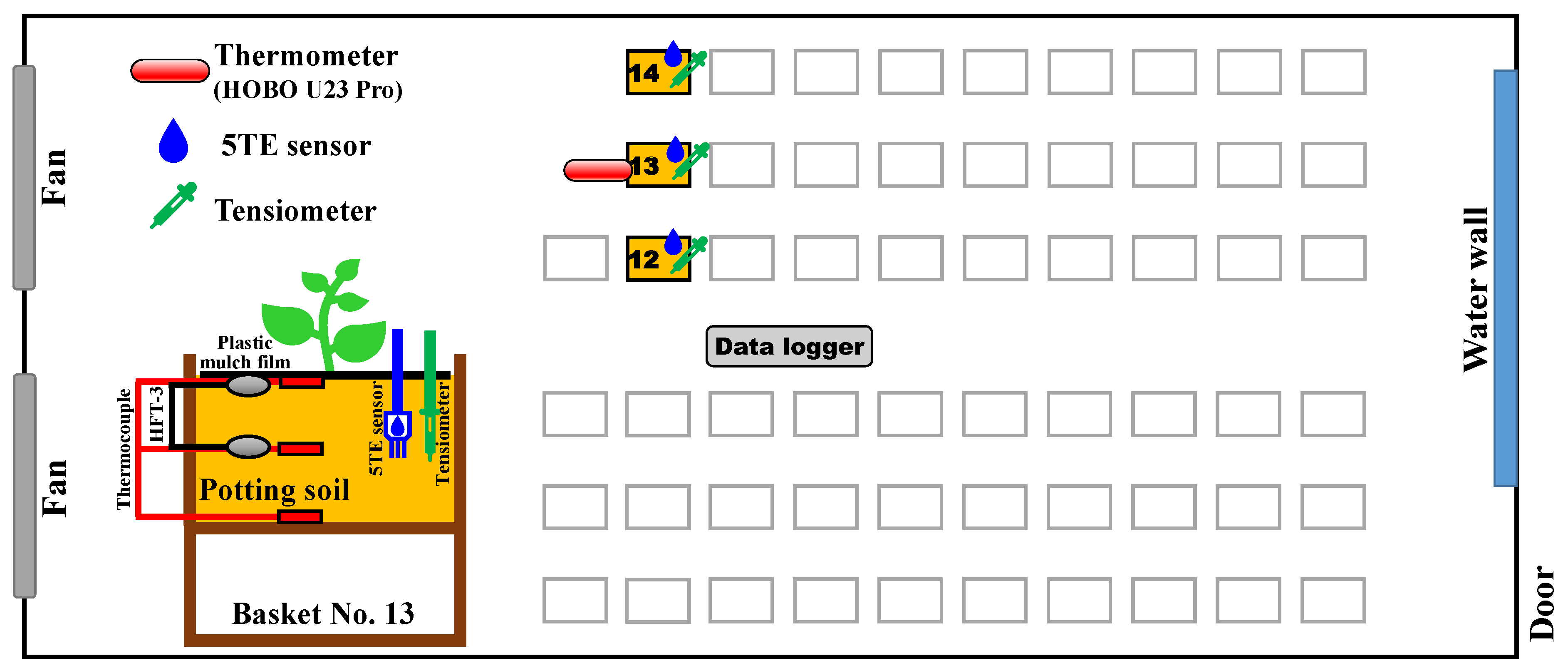
Figure 1. Experimental instrument diagram of the greenhouse. The long-term cherry tomatoes experiment was performed in baskets No. 12, No. 13, and No.14.
Water 12 01176 g001
Figure 2. (a) Soil water characteristics curve of the culture substrate (Sunshine® #5 Natural & Organic Mix) during the drainage stage; (b) Relationship between thermal conductivity and volumetric water content of the culture substrate.
Water 12 01176 g002
Figure 3. Temporal distributions of measured (a) air temperature, (bd) soil temperature, and (eg) volumetric water content for baskets (b,e) No. 12, (c,f) No. 13, and (d,g) No. 14 in the greenhouse during the cultivation period (20 September 2018 to 9 January 2019). The DAT of the X-axis represents the days after transplanting.
Water 12 01176 g003
Figure 4. Soil temperature simulation of Newton’s law of cooling for baskets (a) No. 12 k = −0.306 h−1, (b) No. 13 k = −0.214 h−1, and (c) No. 14 k = −0.221 h−1. Soil temperature simulation by HYDRUS-1D with the measured/empirical parameters in basket (d) No. 13. Soil temperature simulation of the random forest model for baskets (e) No. 12, (f) No. 13, and (g) No. 14. The orange lines are the test set of the measured soil temperature.
Water 12 01176 g004
Figure 5. Simulation accuracy of the random forest model with various training numbers in our study. The accuracy was calculated by dividing the correct number of random forest model into the total number of trainings. The accuracy exceeded 0.9 with more than 250 training numbers.
Water 12 01176 g005
Figure 6. Comparison of the measured and the simulated soil temperature by (a) Newton’s law of cooling, (b) HYDRUS-1D, and (c) the random forest model. The straight slash is a 1:1 line.
Water 12 01176 g006
Figure 7. Soil volumetric water content simulation by HYDRUS-1D with the measured/empirical parameters in basket (a) No. 13. Soil volumetric water content simulation of the random forest model for baskets (b) No. 12, (c) No. 13, and (d) No. 14. The blue lines are the test set of the measured soil volumetric water content.
Water 12 01176 g007
Figure 8. Comparison of the measured and the simulated soil volumetric water content by (a) HYDRUS-1D and (b) the random forest model.
Water 12 01176 g008
Figure 9. The interaction factors used to establish the ICON model with the training set: (a,d,g) air temperature ( T a ), (b,e,h) soil temperature ( T s ), and (c,f,i) volumetric water content (VWC) in baskets (ac) No. 12, (df) No. 13, and (gi) No. 14.
Water 12 01176 g009
Figure 10. Simulation results of the ICON model in baskets (ac) No. 12, (df) No. 13, and (gi) No. 14 for (a,d,g) air temperature ( T a ), (b,e,h) soil temperature ( T s ), and (c,f,i) volumetric water content (VWC).
Water 12 01176 g010
Figure 11. Comparison of the measured and the simulated values by the ICON model for (a) soil temperature and (b) volumetric water content.
Water 12 01176 g011
Figure 12. Simulation performance of models (HYDRUS-1D, random forest model, and ICON model) as compared to the measured data with error bars for (a) soil temperature and (b) volumetric water content. Error bars represent the standard deviation of the measured data.
Water 12 01176 g012
Figure 13. Prediction results from the outdoor air temperature of the weather forecast by (a,b) HYDRUS-1D with the measured parameters, (c,d) the random forest model via the training data, and (eh) ICON model re-established with four factors in basket No. 13 for (a,c,g) soil temperature and (b,d,h) volumetric water content.
Water 12 01176 g013
Table 1. Inputs and outputs of the studied models.
ModelsParametersInputsOutputs
Newton’s law of cooling k = 0.247 ± 0.042 hr−1For temperature: T s ( ξ ) , T a ( ξ ) ,
Δ t = t ( ξ + 1 ) t ( ξ )
I.C.: T s 0 , T a 0
T s ( ξ + 1 )
HYDRUS-1D α = 0.006 cm−1,
n = 2.62 ,
m = 0.62 ,
θ s = 0.72 cm3 cm3,
θ r = 0.05 cm3 cm3,
L = 0.5 ,
K s = 57.02 cm day−1,
Δ z = 10 cm,
b 1 = 2.78 W cm-1 K1,
b 2 = 40.34 W cm1 K1,
b 3 = 8.15 W cm1 K1,
β = 0 ° ,
β T = 5 cm,
S = 0 cm3 cm3 s1,
C p = 1.43 J cm3 K1,
C w = 4.18 J cm3 K1
For temperature: T s ( ξ ) , θ ( ξ ) ,
Δ t = t ( ξ + 1 ) t ( ξ )
I.C.: T s 0 , θ 0
B.C.: soil temperature and matric potential for upper and lower boundaries
T s ( ξ + 1 )
For volumetric water content (VWC):
θ ( ξ ) ,
Δ t = t ( ξ + 1 ) t ( ξ )
I.C.: θ 0
B.C.: matric potential for upper and lower boundaries
θ ( ξ + 1 )
Random forestn_estimators = 100,
max_depth = unlimited,
min_samples_split = 2
For temperature: T a ( ξ ) , T a ( ξ + 1 ) , T s ( ξ )
I.C.: T s 0 , T a 0
T s ( ξ + 1 )
For VWC: T a ( ξ ) ,   T a ( ξ + 1 ) , T s ( ξ ) ,   T s ( ξ + 1 ) , θ ( ξ ) , θ ( ξ 1 )
I.C.: T s 0 , T a 0 , θ 0 , θ 1
θ ( ξ + 1 )
Inferring connections of networks (ICON) M = 2000 ,
N = 3 (simulation) or 4 (prediction),
r = 312 ± 20.1 (for T s ); 313 ± 22.4 (for T a ); 38.7 ± 7.0 (for VWC)
For temperature and VWC: T s ( ξ ) , T a ( ξ ) , θ ( ξ ) ,
forecasted outdoor air temperature as the fourth input factor for prediction stage
I.C.: T s 0 , T a 0 , θ 0
T s ( ξ + 1 ) ,
T a ( ξ + 1 ) ,
θ ( ξ + 1 )
: Initial conditions; : Boundary conditions.
Table 2. Root mean square errors (RMSEs) and Nash-Sutcliffe model efficiency coefficients (NSEs) of the model simulations.
ModelsRMSENSE
Soil Temperature (°C)VWC (cm3 cm−3)Soil Temperature (°C)VWC (cm3 cm−3)
Newton’s law of cooling0.763 ± 0.133-0.905 ± 0.033-
HYDRUS-1D0.4690.0240.9700.626
Random forest0.201 ± 0.0200.008 ± 0.0010.994 ± 0.0010.961 ± 0.014
ICON0.206 ± 0.0060.008 ± 0.0010.994 ± 0.0010.962 ± 0.004
Table 3. Inputs and outputs for converting the forecasted outdoor air temperature to the indoor air temperature for the studied models.
ModelsInputsOutputs
HYDRUS-1DFor air temperature: (linear regression)
forecasted outdoor air temperature: T f o r e c a s t
converted indoor air temperature: T a c o n v e r t
For soil temperature: (linear regression)
T a c o n v e r t
soil temperature of upper and lower boundaries: T s u p p e r and T s l o w e r
Random forestFor air temperature and VWC:
forecasted outdoor air temperature,
24-h time,
ultraviolet index (UVI)
T a c o n v e r t
ICONThe forecasted outdoor air temperature as the fourth input factor
Table 4. RMSEs and NSEs of model predictions.
ModelsRMSENSE
Soil Temperature (°C)VWC (cm3 cm−3)Soil Temperature (°C)VWC (cm3 cm−3)
HYDRUS-1D1.0060.011−0.0200.342
Random forest0.3330.0060.8890.795
ICON1.7010.006−2.8130.850