Abstract
While winter storms are generally common in western Europe, the rarer summer storms may result in more pronounced impacts on lake physics. Using long-term, high frequency datasets of weather and lake thermal structure from the west of Ireland (2005 to 2017), we quantified the effects of storms on the physical conditions in a monomictic, deep lake close to the Atlantic Ocean. We analysed a total of 227 storms during the stratified (May to September, n = 51) and non-stratified (November to March, n = 176) periods. In winter, as might be expected, changes were distributed over the entire water column, whereas in summer, when the lake was stratified, storms only impacted the smaller volume above the thermocline. During an average summer (May–September) storm, the lake number dropped by an order of magnitude, the thermocline deepened by an average of 2.8 m, water column stability decreased by an average of 60.4 j m−2 and the epilimnion temperature decreased by a factor of five compared to the average change in winter (0.5 °C vs. 0.1 °C). Projected increases in summer storm frequency will have important implications for lake physics and biological pathways.
1. Introduction
In our currently warming climate [1], storms are projected to become more common [2] and to increase in strength [3] in many regions, including the Atlantic seaboard of Europe [4]. It is therefore essential to quantify the impact of storms on all natural ecosystems, but especially on lakes which are highly responsive to changes in local weather [5,6]. Storms can affect the flow of energy (heat) in and out of lakes through associated increases in wind speed, lower air temperatures, lower incoming shortwave radiation and increased precipitation. Wind speed is an important component in the transport of momentum, heat and atmospheric moisture [7]. Higher wind speeds increase turbulent mixing within lakes which lowers water column stability and deepens or removes thermoclines [8]. The exchange of heat between lakes and the atmosphere in turn affects a wide range of processes within lakes, including thermal structure, water column stability, thermocline depth [9], nutrient cycling [10], phytoplankton growth [11,12,13] and water turbidity [13,14].
The effect of storms on physical parameters in lakes can be relatively short lived, from days [15], to weeks [13], and can last until autumn turn over [6] or indeed result in multi-annual effects [5]. The same storm can affect different lakes in different ways [16], indicating that lake-based characteristics influence these impacts. These might relate to the characteristics of a storm itself such as wind speed and rainfall, or to characteristics of the lake and its location, such as lake volume, lake area and surrounding topography. Conditions leading up to a storm event may also be significant in predicting the impact. Perga et al., for example, showed that antecedent weather conditions were important in determining storm impact on lake turbidity in alpine lakes [17].
Untangling this web of drivers of storm impacts on lakes can only be achieved by investigating a large number of storms of varying strength and duration, occurring at times when internal parameters within the lake, such as thermocline depth, water temperature and water column stability, are also changing. It requires a long time series of high frequency data on water column temperature profiles, data archives that are scarce in Europe and globally [18]. Single storm events have been investigated before [6,13,15,16,19], some studies have investigated several storms occurring over months or few years [5,17,20,21], but to our knowledge no studies to date have looked at large numbers of storm events over many years in one lake.
In the present study, we investigated the effect of storms on physical conditions in Lough Feeagh, Co. Mayo, Ireland (Figure 1), during fully mixed conditions in winter and in the stratified period in summer. We quantified the changes in a range of lake physical parameters including energy flow (heat fluxes), temperature change, water column stability and thermocline depth. In total, we analysed the impact of 227 storm events on the lake between 2005 and 2017. We hypothesised that the effects on lake physics would be more pronounced with increasing wind speed, longer storm duration and higher rainfall. We also expected that storms with a trajectory along the long axis of the lake would have a larger impact compared to storms that where the main wind direction was perpendicular to the long axis, because Lough Feeagh is a long narrow single basin. Because of the location of Feeagh in western Ireland, close to the Gulf stream, we also hypothesised that storms that came from the ocean would bring air that was warm relative to the lake surface in winter, and vice versa in summer. This added potential for heating of the lake during winter storms, while summer storms were expected to cool down the lake.
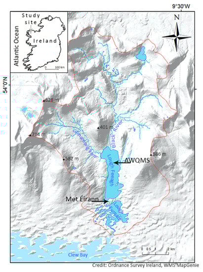
Figure 1.
Location of Lough Feeagh on the west coast of Ireland and the data collection stations. The Automatic Water Quality Monitoring Station (AWQMS) and the Met Éireann station are marked with arrows. The Glenamong river and the Black River enter the lake in the north end.
2. Materials and Methods
2.1. Site Description
The investigation was conducted in the relatively deep (maximum depth 46 m), medium-sized (surface area 3.95 km2) Lough Feeagh, located on the west coast of Ireland (53.94 °N, −9.57 °W). It is the largest lake in the coastal Burrishoole catchment [22]. Lough Feeagh is bathtub shaped (length ~4 km and width ~1 km) and lies along a north–south axis, with the two main inflows, the Glenamong and Black rivers, entering the lake at the northern end. At the southern end of the lake, the Mill Race and Salmon Leap rivers drain into the brackish coastal lagoon Lough Furnace, which drains into Clew Bay and eventually the Atlantic Ocean (Figure 1). High frequency monitoring data were collected from the Feeagh Automatic Water Quality Monitoring Station (AWQMS) which is deployed on a raft moored at the deepest point on Lough Feeagh.
The catchment is dominated by blanket peat and contains only dispersed houses. The main land uses are commercial non-native coniferous forestry, which covers 23% of the catchment, and extensive sheep grazing [23]. The catchment (outlined with red in Figure 1 is 100 km2, catchment for Lough Feeagh is 84 km2) is well defined by the surrounding Nephin Beg mountain range which towers up to 580 m on either side of the elongated lake, but at the northern and southern ends the lake lies exposed to the wind (Figure 1).
The mean annual precipitation was 1652 mm year−1 between 2005 and 2017 at the Newport meteorological station (Met Éireann, unpublished data). Precipitation occurs throughout the year but is generally highest in autumn and winter. The Irish west coast is exposed to the dominant south west (SW) wind direction. Average monthly wind speeds are high at 5.0 m s−1 (range of monthly mean wind speed: 4.5–5.6 m s−1; measured on the AWQMS 2004–2017). The climate is temperate with both mild winters (January mean air temperature 2004–2017: 6.5 °C) and mild summers (July mean air temperature: 14.6 °C; measured on the AWQMS 2004–2017) owing to the influence of the Gulf Stream which transports water of relatively constant temperatures along Ireland’s western coasts.
Lough Feeagh has an average pH of 6.7 and low alkalinity [5,23,24]. It is dystrophic and has medium to high concentrations of coloured dissolved organic matter resulting in brown lake water with low transparency (average Secchi depth 1.6 m). Mean annual total phosphorus (TP) was 6.1 µg L−1 (2017) and total nitrogen (TN) was 430 μg L−1 [25], which is consistent with oligotrophic conditions [26]. Lough Feeagh is almost devoid of submerged vegetation and phytoplankton growth is limited, with chlorophyll a rarely exceeding 3 µg L−1 [6]. The average water residence time in Lough Feeagh is 164 days [5], but residence time is reduced during periods of high precipitation [6]. Lough Feeagh is monomictic, usually stratifying in late spring and remaining stratified until autumn turnover from which time it remains fully mixed until next spring (Figure 2.).
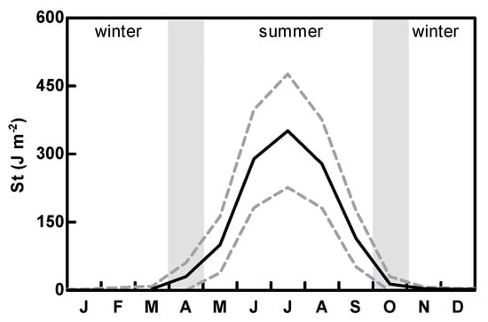
Figure 2.
Schmidt stability (St) in Lough Feeagh in a standard year (based on mean values for 2005–2017). Black line (St) indicates the mean, and dashed lines are ±1 standard deviation. Winter (fully mixed) and summer (stratified) periods are shown. The grey background shows April and October which were omitted from the analysis.
2.2. Meteorological and Lake Datasets
The AWQMS on Lough Feeagh was equipped with a cup anemometer (A100L2-WR, Vector Instruments, Rhyl, United Kingdom), a quantum sensor for PAR light (LI-190-SA, Li-Cor, Lincoln, NE, USA), a platinum resistance thermometer for measuring air temperature (SKH 2012, Skye instruments, Llandrindod Wells, United Kingdom), submerged platinum resistance thermometers (PRTs) at depths of 2.5, 5, 8, 11, 14, 16, 18, 20, 22, 27, 32 and 42 m (PT100 1/10DIN, Lab Facility, Bognor Regis, United Kingdom) and a multi-parameter sonde (Quanta or DS5X, Hydrolab Corporation, Austin, TX, USA) fitted with a temperature sensor deployed at a depth of 0.9 m. All data were recorded locally and transmitted to a computer at the Marine Institute on the shore of Lough Feeagh for storage. The logging interval was every 2 min, except for 2008 and 2009, when the data were logged at 5 min intervals. For the current study, all data were converted to 1 min intervals by linear interpolation. From 2014 to 2017, an additional temperature sensor (TidbiT v2, UTBI-001, Onset Computers, Bourne, MA, USA) was installed at 0.2 m depth, and the data from this sensor were used to check for signals of near-surface stratification. No significant difference was found between temperatures measured at 0.2 and 0.9 m, and so the 0.9 m temperature from the multi parameter sonde was assumed to be a reasonable approximation of surface temperature.
Precipitation, air temperature, relative humidity, wind speed and wind direction at one-minute intervals were retrieved from the Met Éireann automatic weather station (Newport) which is located on the southern shore of Lough Feeagh (Figure 1). The wind speed data from the Met Éireann station (Uland) had very few gaps (1.2% of all data points were missing). The wind speed recorded on the AWQMS (UAWQMS) was assumed to be more representative for conditions on the lake but had more gaps (16.2% of all data points were missing). Therefore, we established the relationship between the two sets of wind speed measurements (UAWQMS, and Uland) for periods when both stations operated, which allowed us to convert wind speeds measured at the Met Éireann station to those measured at the AWQMS and use this to fill gaps in the AWQMS data. The coefficient of determination (r2) for the linear regression was high at 0.76. However, a closer inspection of the data revealed that the relationship between wind speeds on the AWQMS and the land station was nonlinear. Maximum wind speeds were higher but average wind speeds were lower at the Met Éireann station compared to the AWQMS, and a simple height correction [27] for measurements at different altitudes (2.4 m on the AWQMS and 10.0 m over land) was not sufficient to adjust Uland measurements to UAWQMS. Examination of the relationship showed that between wind speeds of 0.00 and 5.95 m s−1 a linear relationship was appropriate (UAWQMS = Uland* 1.1499), and for wind speeds higher than 5.95 m s−1 a 2nd order polynomial was applied (UAWQMS = −0.0145 × Uland2 + 1.027836 × Uland + 1.239455). Corrected wind speed data from the Met Éireann station were then used to fill gaps in the dataset from the AWQMS and the resulting dataset had very few gaps (0.3% of all data points). In addition to local meteorological data, Lamb weather types (LWT) [28], adjusted to Ireland [29], were used. The LWTs are a synoptic climatology tool used for analysing seasonal and annual differences in climate across the British isles [29,30]. With adjustments to centre LWTs over Ireland [29], we used LWTs to describe large scale meteorological flow patterns over Ireland since that might affect storm intensity or impact of individual storms.
In order to calculate the volume-weighted lake temperature, temperature data from the PRTs were related to discrete layers of the total lake volume. Water volume was calculated from a bathymetric table (Marine Institute unpubl. data). The lake was divided into layers which went from the midpoint between two temperature sensors to midway between the next two sensors. Two exceptions were the first layer which went from the lake surface to the midpoint between the first two sensors and the last layer which went from the midpoint between the last two sensors and the lake bottom. Each layer was assumed to have a reversed conical frustum shape. The heights and the areas of each end of the cones were known from the bathymetrical table and so the volume of each layer could be calculated. Since the division into layers was based on where the sensors were placed, each layer contained a thermistor which made it possible to relate each sensor to a known volume of the lake and calculate a volume-weighted average temperature for the lake.
2.3. Lake Physics
Input parameters required for calculations of lake physical parameters (wind speeds (m s−1), water column temperatures (°C), air temperatures (°C), incoming shortwave energy (W m−2) and relative humidity (%)) were averaged to each hour (n = 113952) then Schmidt stability [31], Lake Number [32], u* (or ustar, the water friction velocity due to wind stress [33]) and thermocline depth [33] were calculated using the MatLab© version of Lake Analyser (LA) [33]. Lake Number and u* were recorded as the averages for 3 days before storms, the averages during storms and the averages for 3 days after storms. Lake Number was used to evaluate when stratification was weak relative to wind stress [32,34]. Values lower than 1 are indicative of strong internal seiching and hypolimnetic mixing and the potential for upwelling [19,34].
Schmidt stability is defined as the amount of work required to transform the observed density gradient in the water column into a fully mixed water column with no net gain or loss of heat, thus Schmidt stability serves as a measure of how strong the stratification of the water column is [31,35].
The MatLab© version of Lake Heat Flux Analyzer (LHFA) [7] was used to calculate surface heat fluxes, net incoming short-wave radiation (Qsin), sensible heat flux (Qh), latent heat flux (Qe), incoming long-wave radiation (Qlin), outgoing long-wave radiation (Qlout) and the coefficients associated with the transfer of heat, drag and moisture. Diel values (n = 4748) were calculated subsequently from the hourly output from LA and LHFA. Advective heat fluxes Qadv, the exchange of heat by river inflow and outflow [36], were calculated according to Livingstone and Imboden [37]:
CP is the specific heat of water, is the density of water, Fout is the outflow of water, Tin is the inflow temperature, TW is the lake surface water temperature and AO is the lake surface area. The total heat flux (Qtot) was then calculated as:
Qtot = Qsin + Qlin − Qlout − Qh − Qe − Qadv.
2.4. Storm Detection
The wind energy input, P10 (, [9]), can be used to quantify the input of turbulent energy from the wind into a lake. C10 is the drag coefficient, ρair is the density of air and W10 is the wind speed at 10 m above the water, which are all outputs of the Lake Analyser program [33]. Since P10 is a measure of energy input into the lake it would be intuitive to use this term to detect storms. However, while the cubed term for wind speed in the P10 calculation enhanced peaks in the dataset, it resulted in a very erratic dataset and a much poorer detection of the beginning and end of the storm events thus failing to estimate the correct durations for the storms even when smoothing was applied. Following visual inspection of the storms detected using P10, we decided instead to use smoothed wind speed data as the measure to detect storms. Storms were identified using peak detection in MatLab© on the wind speed dataset (1 min frequency) smoothed by a four-hour running average. Every peak higher than 97.5% of the wind speeds in the smoothed dataset (top 2.5% percentile) were considered to be a storm. The top 2.5% in the smoothed dataset corresponded to wind speeds of >10.6 m s−1.
Using a percentile of wind speeds meant that the wind speed required to qualify as a storm was site specific. Lough Feeagh, due to its location on the Atlantic coast has comparatively high wind speeds. As a comparison, Perga et al. [17] used the top 3% percentile daily wind speed when analysing storm events in Lake Muzelle in the French Alps, which corresponded to a wind speed threshold of just 3.0 m s−1. The average wind speed on Lough Feeagh during the entire 13-year study period was 5.0 m s−1.
To find the duration of each storm, a storm was considered to have started when wind speeds exceeded the average wind speed (2005–2017) for the last time before a peak, and storms were considered to have ended the first time the wind speed dropped below average wind speed again. If the period between storm start and storm end contained more than one peak, only the highest peak was recorded and stored as the peak time for that storm event. This method is different from the mean daily wind speed approach [5,13,17] in which the average diel wind speed is calculated for each day during the study period, and days with average wind speed in a selected top percentile are assumed to include storms. Using that method, a storm that peaks around midnight and lasts only for a few hours in the day before and after its peak might be missed if the wind speeds before and after the storm were relatively low. Our method has four advantages: (i) it does not miss storms that peak around midnight, (ii) it detects relatively short-lived storm events with a calm period before and after, (iii) it considers long storms that may last several days as one event and (iv) it quantifies the duration of storms in hourly rather than diel resolution. This allows quantification of the impact of storms relative to the duration of storms in addition to average or maximum wind speeds.
Storms were grouped into those occurring either during stratified conditions (May–September) or during mixed conditions (November–March). Data for April and October were not used as the conditions were too variable between years for reasonable inter-annual comparisons (Figure 2). Storms that took place early in a year where the lake stratified late, or late in a year where the lake mixed early were also filtered out for our study. Storms that took place during stratified conditions (May–September) are hereafter named summer storms and storms that took place during the fully mixed period (November–March) are called winter storms.
Once storms were identified, key parameters for each storm event were extracted from the hourly data (Table 1). Average diel heat fluxes were collected for three days before the storm, during the storm and for three days after the storm. Diel averages were chosen since there are pronounced diel amplitudes in heat fluxes. So, in order to reasonably compare days against each other, full diel cycles had to be used. This method has the same caveat as described above, that for the first and last day of a storm event it might only have been stormy for a part of the day. If a storm happened within three days after the previous storm, the overlapping heat flux data prior to the second storm, and after the first storm were discarded to prevent these data from being recorded multiple times.

Table 1.
Characteristics of winter and summer storms. Averages given with standard error in parentheses.
Wind directions were recorded both as the average wind direction and the dominant wind direction during each storm. Average wind direction was the average during each storm, calculated using circular statistics, so that the average between two wind directions of 5° and 355° was 0/360° (straight north) rather than 180° (straight south), using the CircStat toolbox for MatLab [38]. For the dominant wind direction, measured wind directions for the duration of the storm were divided into 16 bins of 22.5 degrees each. The interval with the most counts was taken as the direction that the wind came from for the longest time during each storm and recorded as the dominant wind direction.
Fetch is the distance that wind travel over the lake uninterrupted by land [26]. Lough Feeagh is not circular (Figure 1), therefore fetch changed according to wind direction. We manually calculated fetch as the longest measured distance from shore to shore at the given wind direction in 5° intervals from 0° to 360°, and linear interpolation was used between the intervals.
2.5. Statistical Methods
Principal component analysis (PCA) was applied to all explanatory and response variables to visualise which variables were positively and negatively correlated with each other, if there was collinearity, and to get an overview of the data. We used the built-in PCA function “prcomp” in R ver. 3.6.0 [39].
General additive modelling (GAM) with a cubic smoothing regression spline and cross validation was used to determine the relationships between four metrics of change in the lake from pre-storm to post-storm conditions during summer storms. These were: (1) change in Schmidt stability, (2) change in surface water temperature; (3) change in the whole lake temperature; (4) change in the depth of the thermocline. The independent variables were: storm duration, average wind speed, average wind direction, average wind gust speed, thermocline depth at start of storm, fetch and average air temperature. The data analysis was carried out using the mgcv [40] and nlme [41] packages in R [39]. The sequence of the analysis was guided by the protocol of Zuur et al. [42]. The independent variables were first checked for any collinearity and no variables with a correlation coefficient of greater than 0.5 were included in the same model. Residuals of the model were checked for any breach of the assumption of equal variance using the gam.check function in mgcv. The final model was checked for any breach of the assumption of independence by plotting autocorrelation functions of the model residuals.
T-tests were used to compare datasets against each other for differences in mean values. Welch’s T-test was used in cases when variations were unequal between datasets. T-tests were performed in GraphPad Prism 5 (GraphPad Software Inc. San Diego, CA, USA).
3. Results
3.1. Wind Direction and Storm Characteristics
A total of 227 storms (mean 17.5 storms year−1, S.E = 1.55) were identified in the thirteen years of the study period, 51 during summer (mean 3.9 storms year−1, S.E = 0.46) and 176 during winter (mean 13.5 storms year−1, S.E = 1.50). The maximum number of storms in any one year was 29 (7 summer and 22 winter storms) in 2007. Summer storms occurred in all years between 2005 and 2017, range was between 1 (2011) and 7 (2007).
The wind direction over the total study period was predominantly in directions from southerly through to westerly (Figure 3 and Table A1). Breaking down the dominant wind directions during storms showed that 86% of the summer storms and 77% of the winter storms had a westerly component and around half of all the storms had a southerly component (Figure 3 and Table A1). Less than 40% of the storms had a northerly component and easterly winds were uncommon during storms. On average during all storms, the wind direction was 237° in winter and 248° in summer, which in both cases translate into west south-westerly wind. There was, however, a difference between summer and winter storms, with summer storms having a lower westerly component, while winter storms had a lower south-westerly component (Figure 3 and Table A1).
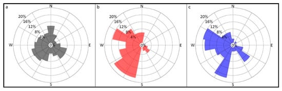
Figure 3.
Wind roses. Grey rose (a) show the entire dataset, one-minute data from 2005 to 2017 (n = 6,837,120). Red rose (b) shows the dominant wind directions during summer storms (n = 51). Blue rose (c) shows the dominant wind directions during winter storms (n = 176).
The Lamb weather types (LWTs) for Ireland for the study period showed a pattern consistent with that derived from the wind direction data, with a majority of westerly (38%–44%) and southerly (19%) types (Figure 4). During summer storms, cyclonic LWTs had approximately the same frequency as southerly LWTs, while days assigned to northerly types accounted for 15% and days with anti-cyclonic patterns for about half of that (7%). Easterly LWTs did not occur at all during summer storms. For winter storms, cyclonic LWTs decreased and anticyclonic types increased (both were about 12%), while northerly types decreased to 10% and there was only a small number of days with easterly LWTs (Figure 4, white columns).
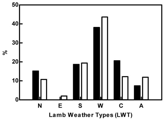
Figure 4.
Percentage contribution of Lamb weather types. LWTs centred over Ireland during storms in summer (black columns) and winter (white columns). northerly (N), easterly (E), southerly (S), westerly (W), cyclonic (C) and anti-cyclonic (A) for the period 2005–2017.
Both average wind speed (p < 0.001) and maximum speed (p < 0.001) were significantly higher during winter storms (8.6 and 16.6 m s−1) compared to summer storms (8.2 and 15.0 m s−1) (two-sample unpaired t-test). However, although the average winter storm was numerically longer (54 h, S.E. = 2.5) than the average summer storms (46 h, S.E. = 3.0), the difference was not significant. The shortest summer storms lasted for 15 h, while the longest lasted just under 4 days (92 h). The shortest winter storm lasted just 9 h while the longest lasted nearly 8 days (186 h). We detected no significant trend of change in duration (gam, R2 adj. = 0.006; edf. = 1, p = 0.122) or average wind speed (gam, R2 adj. = 0.010; edf. = 1, p = 0.073) of storms over the 13-year study period.
3.2. Changes in Water Column during Storms
The storms varied in duration and intensity and in the amount of precipitation (Figure 5). The shortest summer storm, July 2010 (Figure 5, panels a1–a3), for example, had high wind speeds, 16.2 m s−1, but it lasted only 15 h. This storm had an abrupt impact on Schmidt stability, which dropped immediately, but the impact was short lived and water column stability was restored within 24 h. The July storm of 2011 (Figure 5, panels b1–b3) lasted longer, 73 h, and it resulted in a profoundly lowered Schmidt stability. Although Schmidt stability slowly started increasing again immediately after the storm, the lake did not regain the pre-storm levels of stability again that summer. The storm of June 2012 (Figure 5, panels c1–c3) was a medium duration storm (40 h) and it had the highest rain fall of the example summer storms (47.7 mm). The immediate impact on Schmidt stability of the 2012 storm was comparable to that of the long duration storm of 2011, but after one month, the water column regained its stability. In the 2010 storm, the thermocline depth at the start of the storm was at 19 m while at the start of the 2011 and 2012 storms the depths of the thermocline were only 10.5 and 7.5 m respectively.
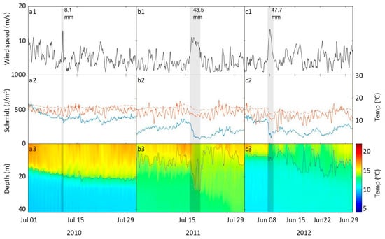
Figure 5.
Examples of summer storms. Storm July 2010 (a1–a3), storm July 2011 (b1–b3), and storm June 2012 (c1–c3). Black line in top panels (a1–c1) are 4h average wind speed in m s-1. Blue lines in panels (a2–c2) are Schmidt stability (J m−2), red lines in panels (a2–c2) are air temperatures (°C), dashed lines are surface water temperatures and the full lines are the air temperatures. Isopleth plots in panels (a3–c3) are the temperature profile in the lake and the grey lines shows the location of the thermocline. Vertical greyed areas indicate the storm durations, next to each storm is the amount of rainfall for the storm duration (mm).
For comparison, two examples of winter storms are shown in Figure A1. Storm Imogen was a winter storm that occurred in early February 2016 and, with a duration of over four days (102 h), it lasted longer than any of the summer storms. Storm Imogen had maximum wind speeds of 16.5 m s−1 and delivered 96 mm of rain. However, the impact on the water column was negligible as the water column was well mixed even before the storm. In fact, Schmidt stability increased very slightly from 2.64 to 3.49 J m−2 during Storm Imogen. The unnamed storm in late February of same year (Figure A1) lasted 58 h, about half the duration of Storm Imogen, but had higher wind speeds, up to 20.6 m s−1. Similar to storm Imogen, this storm had very little impact in the water column.
The direction of the difference between surface water temperature and air temperature during storms changed seasonally. During summer storms, the air temperature was on average 1.5 (S.E. = 0.12) °C colder than the surface water temperature, whereas in winter, the air was on average 0.5 (S.E. = 0.14) °C warmer than the lake surface. This temperature deficit did not, however, result in heating of the lake in winter storms. Both whole lake temperature and surface water temperatures decreased by 0.1 °C (S.E. whole lake = 0.02, S.E. surface = 0.03) during winter storms. In summer when the lake was stratified, the average whole lake temperature decrease during storms was also 0.1 (S.E. = 0.03) °C, but the surface water temperature decrease was 5-fold larger (0.5 °C, S.E. = 0.08).
During winter storms when the water column was well mixed, there was no distinct thermocline, and this did not change during storms. Schmidt stability did decrease slightly during storms in winter (0.4, S.E. = 0.33 J m−2) (Table 1). Due to the well-mixed conditions in the water column in winter, the lake number remained on average below 1 (0.54, S.E. = 0.20), but during storms it still decreased by approximately an order of magnitude to 0.07 (S.E. = 0.03).
During summer, the impact of storms on the water column was pronounced. On average the thermocline was moved 2.8 (S.E. = 0.56) m deeper into the water column. Simultaneously, Schmidt stability decreased by 24%, from an average of 255.8 (S.E. = 21.4) J m−2 to an average of 195.3 (S.E. = 19.5) J m−2 (Table 1). The lake number also decreased during storms. In the periods prior to summer storms, the average lake number was 12.3 (S.E. = 1.33) and only on 4% of the days analysed before storms did the lake number drop below 1. In contrast, during storms the average lake number was an order of magnitude lower at 1.7 (S.E. = 0.14) and on 25% of the days during storms it dropped below 1. After summer storms, the average lake number increased again to 13.0 (S.E. = 1.78) but there was still 10% of the days after storms when the lake number was below 1. During summer storms, water friction velocity due to wind stress (u*) also increased by 81% from 0.69 cm s−1 (S.E. = 0.03) to 1.25 cm s−1 (S.E. = 0.01). During winter storms, u* increased by 52% from 0.86 cm s−1 (S.E. = 0.02) to 1.31 cm s−1 (S.E. = 0.01).
3.3. Rainfall
The average rainfall for the summer storms was 15.1 mm, which was roughly one percent of annual total rainfall. But the range in the storm associated rainfall was large and, in some instances, storms brought very heavy rainfall. For example, 96.0 mm was recorded during Storm Imogen, which lasted from the 5th to 9th February 2016 (Figure A1). This rainfall was equal to 71% of an average month of February (2005–2017) precipitation, or 6% of the annual precipitation in 2016. During an unnamed summer storm that occurred between the 7th and 9th of June 2012 (Figure 5 c1–c3), 47.7 mm rainfall was recorded, accounting for 3% of the annual rainfall of 2012 or 51% of an average June (2005–2017) precipitation.
3.4. Storm Impacts on the Lake
Plotting explanatory and response variables together in a PCA plot produced an overview of what separated summer and winter storms. We included the explanatory variables: max speed, average wind speed, storm duration, dominant wind direction, depth of the thermocline at the beginning of storms, fetch, u* and lake number, alongside the response variables: change in whole lake temperature, change in surface water temperature, deepening of the thermocline and change in Schmidt stability, into the PCA (Figure A2). Summer and winter storms formed two separate clusters with winter storms overlapping summer storms in part. The eigenvectors separating the two clusters were deepening of the thermocline, Lake number, pre-storm depth of the thermocline, change in Schmidt stability and change in surface water temperature. Wind speed and u* were almost parallel which is expected since the amount of friction velocity due to wind speed is closely related to wind speed. The eigenvectors wind direction and storm duration were also very similar.
General additive modelling showed that storm duration, storm average wind speed and the initial pre-storm thermocline depth (a measure of pre-storm conditions in the lake) contributed significantly to explaining both the change in Schmidt stability (R2 adj. = 0.66) and the change in surface water temperature (R2 adj. = 0.77) during summer storms (Table 2). For both of these response variables, the relationships to storm duration and wind speed were generally negative—that is, longer storms and higher wind speeds resulted in greater decreases in Schmidt stability and surface water temperature (Figure 6). The relationships to the pre-storm thermocline depth were generally negative: when the thermocline was deeper at the start of the storm, there was a smaller decrease in Schmidt stability and in surface water temperature. When the thermocline was close to the surface before a storm (at 4 to 15 m) the biggest decreases was observed in the response variables and when the pre-storm thermocline depth was greater than 15 m the impacts were generally much smaller. The extent to which the thermocline deepened during a storm was generally positively related to storm duration and average wind speed, and negatively related to the initial thermocline depth (Figure 6, Table 2). Surprisingly, on its own, storm duration, rather than average wind speed, was the variable that explained the largest percentage of deviance in the change in Schmidt stability (R2 adj. = 0.28; edf. = 1, p < 0.0001), deepening of the thermocline (R2 adj. = 0.23; edf. = 1, p = 0.0002) and the change in the surface water temperature (R2 adj. = 0.18; edf. = 1, p < 0.0001).
Table 2.
General additive models for pre- to post-storm change in (1) Schmidt stability, (2) surface water temperature, (3) deepening of the thermocline and (4) change in whole lake temperature, for summer storms (edf. = estimated degrees of freedom) (n = 49).
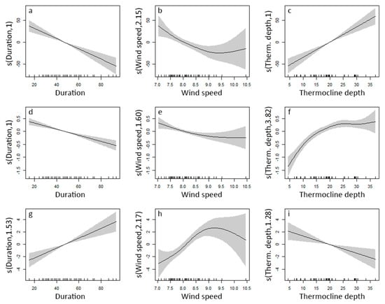
Figure 6.
General additive model smoothers. Panels (a–c) show the components of the gam for explaining changes in Schmidt stability. Panels (d–f) show the components of the gam for explaining changes in surface water temperature. Panels (g–i) show the components of the gam for explaining changes in thermocline depth. The numbers on the x-axes are the estimated degrees of freedom (edf), an edf of 1 is a linear model, numbers higher than 1 show various degrees of non-linearity.
Storm direction was the only variable that was significant for change in the whole lake temperature during summer storms, and it only explained 15% of deviance (R2 adj. = 0.15). The relationship was linear, negative, and spanned a range that included positive changes (maximum +0.2 °C) and negative changes (minimum −0.6 °C). The small increases in whole lake temperature were mainly associated with storms with a direction of between 90 and 200 degrees (easterly through to south-southwesterly), while decreases in whole lake temperature were mainly associated with storms coming from directions between 270 and 360 degrees (westerly through to northerly).
3.5. Heat Fluxes
In summer, the mean total heat fluxes (Qtot) were similar before storms (12.0 W m−2, S.E. = 7.14) and after storms (9.0 W m−2, S.E. = 6.64). Both before and after storms Qtot was positive—that, is the lake was, on average, heating up, but with a large variance around this average. However, during summer storms, the total heat fluxes dropped significantly (one-way ANOVA, p < 0.0001) to −33.0 W m−2 (S.E. = 5.57), the negative value indicating a cooling of the lake. After this Qtot then increased significantly again (one-way ANOVA, p < 0.0001) and became positive (9.0 W m−2) as the lake once again heated up. In winter, total heat fluxes did not differ significantly (one-way ANOVA with Tukey’s post hoc test, p = 0.73) before (−35.7 W m−2, S.E. = 5.44), during (−41.2 W m−2, S.E. = 4.19) or after storms (−40.2 W m−2, S.E. = 4.30), and in all cases, the negative values indicated that the lake, on average, was cooling down (Figure 7, Table 3).
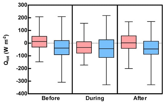
Figure 7.
Diel total heat fluxes (Qtot) before, during and after storms in summer (red) and winter (blue). Negative values result in a cooling of the lake. In summer, a period of general heating, storms cause significantly negative total heat fluxes, resulting in a cooling of the lake. Whiskers show the dataset ranges.
Table 3.
Average values for surface and advective heat fluxes. Average incoming long-wave radiation (Qlin), net incoming short-wave radiation (Qsin), sensible heat flux (Qh), latent heat flux (Qe), outgoing long-wave radiation (Qlout), advective heat fluxes (Qadv) and total heat fluxes (Qtot) before, during and after winter and summer storms on Lough Feeagh between 2005 and 2017, standard error given in parentheses. All units are W m−2. Positive values indicate heating of the lake and negative values represent cooling fluxes. The sum of the heatfluxes (Qtot) is given in bold.
The difference between the mean total heat flux before summer storms and during those storms was driven primarily by increased loss of heat through both of the turbulent heat fluxes (sensible heat (Qh) and latent heat (Qe)) which together increased by an average value of 34.3 W m−2, from 71.0 (S.E. = 4.40) W m−2 before storms to 105.3 (S.E. = 4.34) W m−2 during storms. Qsin was numerically lower during storms compared to before and after storms (Table 3), but the difference was not statistically significant.
Overall, incoming (QLin) and outgoing (QLout) longwave radiation remained the largest components of the heat budget both in summer and winter. However, neither of these changed before, during or after storms, either in winter or summer, Table 3. The transfer coefficients for heat (Ch), humidity (Ce) and momentum (Cd) all increased during storms both in winter and summer. The largest change was in mean Cd value which increased from 1.61 × 10⁻³ (S.E. = 9.10 × 10⁻⁶) to 1.78 × 10⁻³ (S.E. = 1.27 × 10⁻⁵) during summer storms and from 1.60 × 10⁻³ (S.E. = 1.67×10⁻⁵) before winter storms to 1.77 × 10⁻³ (S.E. = 8.74 × 10⁻⁶) during winter storms. In summer storms, Ce and Ch both increased from mean values of 1.62 × 10⁻³ (S.E. = 9.33 × 10⁻⁶) to 1.64× 10⁻³ (S.E. = 4.40 × 10⁻⁶) during storms, while during winter storms the increases were from 1.53 × 10⁻³ (S.E. = 1.33 × 10⁻⁵) to 1.58 × 10⁻³ (S.E. = 4.62 × 10⁻⁶). In winter, the sensible heat fluxes were close to zero both before (1.0 W m−2, S.E. = 1.62) during (5.2 W m−2, S.E. = 1.32) and after storms (−2.1 W m−2, S.E. = 1.25), and the change from positive to negative mean values was not significant.
The advective heat fluxes (Qadv) were on average negative, meaning that there was a net loss of heat from the lake resulting from the inflows and outflow of water combined. During winter the advective heat flux was on average in the same order of magnitude as the sensible surface heat flux and there were no significant differences in advective heat fluxes before, during and after storms (mean values of −3.6 (S.E. = 0.80), −4.0 (S.E. = 0.68) and −3.0 (S.E. = 0.72) W m−2 respectively). In summer, the sensible heat fluxes increased while the advective heat fluxes remained on the same magnitude as during winter. However, advective heat fluxes were significantly more negative during summer storms (mean −7.6 W m−2, S.E. = 0.83) compared to before the storms (mean −4.6 W m−2, S.E. = 0.54) (Mann-Whitney two-tailed, P = 0.04, df. = 224). They remained numerically larger after storms (−6.8 W m−2, S.E. = 0.82) compared to before storms, but this difference was not significant (Table 3). The range for advective heat fluxes was between −84.5 and 6.1 W m−2 during summer storms and between −54.4 and 32.2 W m−2 during winter storms.
Examples of three summer storms shown in Figure 5 experienced some of this diversity in advective heat fluxes. The July storm of 2010 (Figure 5, a1–3) did not have an impact on advective heat fluxes. The average advective heat fluxes three days before the storm was −4.90 W m−2, during the storm it was −4.01 W m−2 and the three-day average after the storm was −3.26 W m−2. But for the other two example storms (Figure 5, b1–3 and c1–3) the advective heat fluxes increased in magnitude during storms. For the July storm 2011 (Figure 5 b1–3) the three-day average before storms was −0.90 W m−2, the average during the storm was −15.13 W m−2 and the average for three days after the storm was −3.23 W m−2. A similar pattern was observed during the June storm of 2012 (Figure 5, c1–3). Three days before the storm, the average advective heat flux was −3.20 W m−2, it increased during the storm to −18.08 W m−2 and after the storm it became slightly positive at 0.22 W m−2. During the winter storms shown in Figure A1, there was no clear pattern in advective heat fluxes. During the three-day period before Storm Imogen the average advective heat flux was −6.70 W m−2. This increased to −9.16 W m−2 during the storm but it then doubled to −18.49 W m−2 during the three days after the storm. For the other but unnamed storm also in Figure A1, the three-day average before the storm was −3.89 W m−2; it dropped to almost zero during the storm (−0.70 W m−2) and became slightly positive after the storm at 2.70 W m−2.
4. Discussion
The projected increases in the frequency and magnitude of storms in the coming decades has implications for a range of physical and biogeochemical processes in lakes. The dominance of westerly and south-westerly winds during the storms that we described for Lough Feeagh reflect its location on the very western edge of Europe and the patterns of deep, low pressure systems in this region. This location also means, as we have shown, that Lough Feeagh is subject to many storms every year and therefore may represent future conditions at other currently calmer sites if the projected increases in storm magnitude and frequency occur [2,3]. We have also shown that although less frequent than winter storms, summer storms occur in all years at this site. Moreover, summer storms had average durations that were similar to winter storms and average wind speeds that were only slightly lower. The summer storms resulted in temperature decreases in the surface water of up to 3.2 °C, and a rapid loss of stability, effects that would have implications for many biogeochemical processes in the lake. However, while wind speed was a significant driver of these changes, it was storm duration that had the greatest influence.
Projected temperature increase in the North Atlantic ocean could result in storms in the region becoming both more frequent and more powerful in the future [19]. The projected increase would have profound implications for physical parameters such as stratification, mixing, thermocline depth in lakes which in turn impact many biological and chemical parameters, such as distribution of nutrients [43,44], phytoplankton [45], zooplankton communities and composition [44,46], microbial communities [46], exchange of dissolved gasses with the atmosphere [47] and ecosystem metabolism [27]. In turn these processes determine availability of dissolved oxygen and finally what parts of the water column can be utilized by zooplankton [48] and fishes [49]. Because of the projected increases in storm frequency and intensity, understanding and quantifying the effects of storms on lake physics has now become important. We have quantified the impact of hundreds of storms of various magnitudes on a medium-sized, moderately deep and humic lake with a temporal resolution of hours rather than days.
During the summer storms, we found that Schmidt stability, thermocline depth and Lake Number all decreased significantly in Lough Feeagh. Our analysis allowed a quantification of these changes over many storms. For example, on average, the surface waters experienced a temperature loss of −0.5 °C during summer storms, and the temperature decrease in the surface water was also 5-fold larger during summer storms compared to winter storms, despite the total heat fluxes being comparable. It is likely that this loss of heat reflected the mixing of colder hypolimnetic water into the epilimnion as the thermocline deepened during the storm. Supporting this, we found Lake Number values that were frequently below 1 during the storms, indicating that internal seiching and upwelling events may have added volumes of cold hypolimnetic water into the epilimnion. In summer the frequency of Lake Numbers below 1 increased more than 6 fold during storms. After storms, the frequency of low lake numbers also remained more than double compared to before storms which is a result of the weaker water column stability.
The exchange of water between the epilimnion and hypolimnion has important implications for the biology in lakes [50,51]. During stratification, metabolic substrates and nutrients can become depleted in the epilimnion due to productivity in these warm and well illuminated waters. In the dark and cold hypolimnion, respiration dominates and there is a release of nutrients and a depletion of oxygen. Dead organic material continuously precipitates from the surface waters and is respired in the bottom waters [26,46]. A catastrophic storm event may break down the thermocline entirely and mix in nutrients and CO2 from the hypolimnion into the epilimnion [15,16]. More moderate storm events may allow smaller amounts of substances to be exchanged between the hypo- and epilimnion by deepening the thermocline, mixing of hypolimnetic water into the epilimnion, initiating internal seiching and causing upwelling events [16]. Transport of nutrients into the surface water stimulate autotrophic growth [43].
We found that the whole-lake average temperature decreased by an equal amount (0.1 °C) during storms both in summer and in winter. However, during winter storms values water column stability were close to zero even before storms occurred, consequently did not change systematically during storms. The well-mixed conditions during winter resulted in Lake Numbers almost constantly below 1, but during storms they decreased even further by almost an order of magnitude suggesting that the winter storms caused increased mixing in the entire water column.
Unsurprisingly, average wind speed during the storms was included in all models explaining changes in Schmidt stability, surface water temperature and thermocline depth. It was more unexpected that storm duration was also included in all the models explaining changes in Schmidt stability, surface water temperature and thermocline depth, highlighting the importance of estimating the duration of storm events. These results indicate that a better estimation of future changes in storm duration would help to further our understanding of the impact of storms on the physical environment in lentic water bodies. It was also notable that we found no trend in storm duration over the 13-year period studied; even longer time series may be needed to identify such trends. The final parameter that our analysis showed was significant in explaining the physical parameters was the pre-storm thermocline depth. This is obviously not a driving parameter as such, but rather one explaining the starting conditions which heavily influence the extent to which a lake will be impacted during a storm event. When the thermocline was located deeper in the lake at the start of a storm, the large volume of the surface mixed layer dampened the impacts of storms; and vice versa, when the thermocline was closer to the surface at the beginning of a storm, a comparatively small volume of water was affected by the storm, and the effects were more pronounced.
Volume-weighted whole lake temperature is unaffected by heterogeneous temperatures in the water column as each sensor is related to a specific volume and then averaged [52,53]. This was supported by our analysis as thermocline depth was not significant in the optimum general additive model for change in whole lake temperature. In fact, none of the parameters indicative of storm intensity, wind speed, gust speed, rainfall or duration explained deviance in the whole lake temperature change. Only storm direction was significant, but the deviance explained was relatively low at 15%. It was somewhat unexpected that wind direction was not significant in explaining storm induced changes on Schmidt stability, surface water temperature or thermocline depth given the situation of the lake between two mountains to the east and west while it is exposed to the wind from the north and south. Indicated by the PCA analysis (Figure A2), however, wind speed and wind direction are both in the same upwards direction, and the wind speed eigenvector is more than twice the magnitude of the wind direction. So, any effect of direction might be masked by wind speed. Wind direction, however, was not significant in explaining wind speed.
Heat Fluxes during Storms
Storms most often came from the Atlantic Ocean, where the Gulf Stream transports water of relatively constant and mild temperatures close to the Irish west coast [54]. We had hypothesised that winter storms would therefore bring warmer air masses to the Irish coast and could have a warming effect on Lough Feeagh. We did find that winter storms brought warmer air relative to the lake surface and conversely colder air relative to the lake surface in summer. Warmer air brought in during winter did not, however, result in a heating of the lake. While there was a positive sensible heat flux (heating of the lake), this was countered by an even larger increase of the latent heat flux (cooling of the lake). This combined with a decrease in incoming shortwave radiation during storms resulted in a net cooling of the lake during winter storms, despite the warmer air brought in with the storm. During winter the decrease in surface water temperature was the same as whole lake temperature loss, which was a consequence of the well-mixed conditions and meant that any change of temperature was distributed evenly in the entire water column. During summer, a period of general heating of the lake, storms resulted in a significant cooling that was of the same order of magnitude as during winter storms. While the whole lake temperature loss during summer storms was similar to that during winter storms, the surface water temperature loss was disproportionally large.
Consistent with cooling of the lake during winter, the total heat fluxes were negative both before, during and after storms (Figure 7, Table 3). During summer, a period during which the lake is generally warming, storms brought on a significant cooling with negative total heat fluxes. The negative total heat fluxes during summer storms were in the same order of magnitude to the negative total heat fluxes on normal non-stormy winter days. However, summer storms occurred during stratified conditions, during which they caused a deepening of the thermocline resulting in mixing in of colder water below the thermocline into the well-mixed layer above, this combined with heat loss across the surface and a loss of heat to the advective fluxes resulted in the 5-fold greater temperature decrease in the surface waters during summer compared to winter.
Over the entire study period, Lough Feeagh had a constant advective loss of heat caused by, on average, colder water entering the lake through the inlets and warmer water leaving through the outlets. Our results provide insights into the dynamics of advective heat fluxes during multiple storms, especially those that occur in summer. Although the advective heat flux (Qadv) was comparatively small (2–3 orders of magnitude smaller than the incoming shortwave radiation (Qsin) and three orders of magnitude smaller than the longwave radiative fluxes (Qlin and Qlout)), a pattern was observed during summer storms when the advective heat fluxes increased in magnitude causing an increased loss of heat. Streams have been shown to increase in flow and decrease water temperature in response to summer precipitation events [55], which explain the observed pattern in advective heat fluxes. The range of the advective heat fluxes in Lough Feeagh was high and, in few instances, they increased by an order of magnitude during storms. In such events, as described for the two summer storms of 2011 and 2012, the advective heat fluxes was a substantial component of the overall heat budget for Lough Feeagh.
While, on average, the influx of water from the inlets might have had a limited impact on the heat budget, it could still play an important biological role in the lake. Such events have potential to wash both particulate and dissolved substances from the catchment into the lake as described in other studies from the catchment [5,6,23,24,56]. The allochthonous carbon inputs that come into the lake with such events would be particularly important for the biology in the lake [57]. Since the Burrishoole catchment where Lough Feeagh is situated is dominated by peaty soils, it is also possible that these pulses in coloured dissolved organic matter would contribute to the typical light limitation of autotrophs in this humic lake [58].
The cooling of the surface waters during summer storms did not result in increased heat fluxes in the period immediately following the storms. We had hypothesised that the cooling of the surface water would result in a steeper gradient between air and water temperatures, with resulting increased transfer coefficients for heat. However, we found no increase in the total heat fluxes in the days following summer storms. This might be because the weather fronts that often accompany storms typically bring a change in the local weather, and so the small changes in water temperature could be countered by much larger changes in, primarily, air temperature, cloud cover and in coming shortwave radiation.
5. Conclusions
Our study is the first to describe in detail what happened to the physical structure in a humic lake during multiple storms, especially those that occur during summer when the impacts on the lake physics were greatest. We found that the surface water temperature decreased 5 fold during summer storms compared to winter storms. Moreover, we have shown that the total heat fluxes during summer storms were negative and of the same order of magnitude as those during winter storms. Summer storms changed the thermal structure of the water column by significantly cooling surface water, lowering Schmidt stability, deepening or removing thermoclines and lowering lake numbers. We also showed that these impacts could be predicted by a combination of storm duration, wind speed and the pre-storm depth of the thermocline.
The impacts of storms effects, which we described here, have implications for lake biology in a changing climate where storms are predicted to become more frequent in Western Europe. Based on our results, and in a climate with more summer storms, we predict that Lough Feeagh would be less likely to remain seasonally stratified and may change from being predominantly monomictic to more polymictic, mixing more frequently through the summer period. This effect, however, may to some degree be countered by increasing temperatures which will act as stabilising force on the lake [59], the increase in temperature anticipated by IPCC [1] has been predicted to impact very large lakes to mix less frequently in-part due to absence of winter ice and more stable water columns in summer [60].
While a decrease in temperature by 0.5 °C itself may not be a dramatic change for most organisms in the lake, the lowered stability of the water column, the deepening or removal of thermocline and the upwelling of hypolimnetic water may be of profound importance for the ecosystem as a whole as it alters and enhances pathways for nutrient and carbon recycling within the lake. We found that the impacts on the water column could be relatively short lived but sometimes persisted through the rest of the summer until autumn turnover mixed the entire water column. Storms then have implications for the physical environment within the lake for days, weeks or even months following the event.
Author Contributions
This study was jointly conceived and carried out by M.R.A., E.d.E., M.D., R.P. and E.J. Data collection was carried out by E.d.E. and M.D. and facilitated by R.P. The manuscript was written by M.R.A., revised by M.R.A., E.d.E. and E.J. and approved by all authors. All authors have read and agreed to the published version of the manuscript.
Funding
This project (Grant-Aid Agreement No. PBA/FS/16/02) is carried out with the support of the Marine Institute and is funded under the Marine Research Programme by the Irish Government.
Acknowledgments
The authors wish to thank Joshka Kaufmann, R. Iestyn Woolway, Karl Philips and the participants of the BEYOND2020 project for constructive feedback during the analysis and writing phase of this study. Joseph Cooney, Michael Murphy, Pat Nixon, Pat Hughes and Davy Sweeney of the Marine Institute, maintained the Feeagh AWQMS over the study period, and their contribution is gratefully acknowledged.
Conflicts of Interest
The authors declare no conflict of interest.
Appendix A

Figure A1.
Examples of two winter storms. Storm Imogen early February 2016 and unnamed storm late February 2016. Black line in top panel a1 are 4 h average wind speed in m s−1. Blue lines in panel a2 are Schmidt stability (J m−2), note the different scale on left y-axis in a2 compared to summer storm examples, red lines in panel a2 are air temperatures (°C), dashed lines are surface water temperatures and the full lines are the air temperatures. Isopleth plots in panel a3 are the temperature profile in the lake and the grey lines shows the location of the thermocline, when one was present. Vertical greyed areas indicate the storm durations, next to each storm is the amount of rainfall for that storm (mm). White area in panel a3 indicates no data. Consistently blue colours with both depth and time in a3 show the well-mixed and low temperatures in the entire water column typical of winter conditions in Lough Feeagh.

Figure A2.
Principal component analysis (PCA) plot. PCA analysis of summer storms (red dots and surface) and winter storms (blue dots and surface). Explanatory variables noted with small font size and response variables highlighted with large font size and bold text.
Table A1.
The dominant wind directions for winter (n = 176) and summer (n = 51) storms and the wind directions for the entire 13-year period (n = 6,837,120). Bottom section breaks the directions into the four corners and show the percentage of storms that has that component in them (e.g., a storm with a dominant direction from “Northwest” have both a northerly and a westerly component, therefore summing up the percentages comes to more than 100%).
| Direction | Winter Storms (%) | Summer Storms (%) | Entire Period 2005–2017 (%) |
|---|---|---|---|
| North | 2.3 | 5.9 | 9.7 |
| North-northeast | 0.0 | 0.0 | 5.0 |
| Northeast | 1.1 | 0.0 | 1.9 |
| East-northeast | 0.0 | 0.0 | 2.0 |
| East | 0.0 | 0.0 | 4.0 |
| East-southeast | 4.5 | 2.0 | 7.9 |
| Southeast | 10.2 | 3.9 | 8.0 |
| South-southeast | 2.3 | 2.0 | 5.1 |
| South | 2.3 | 0.0 | 3.5 |
| South-southwest | 17.6 | 17.6 | 8.0 |
| Southwest | 7.4 | 17.6 | 9.5 |
| West-southwest | 9.1 | 11.8 | 9.8 |
| West | 14.8 | 7.8 | 8.0 |
| West-northwest | 15.9 | 15.7 | 6.8 |
| Northwest | 6.3 | 9.8 | 5.0 |
| North-northwest | 6.3 | 5.9 | 5.8 |
| Northerly | 31.8 | 37.3 | 36.3 |
| Easterly | 18.2 | 7.8 | 33.9 |
| Southerly | 53.4 | 54.9 | 51.7 |
| Westerly | 77.3 | 86.3 | 52.9 |
References
- Frieler, K.; Lange, S.; Piontek, F.; Reyer, C.P.; Schewe, J.; Warszawski, L.; Zhao, F.; Chini, L.; Denvil, S.; Emanuel, K. Assessing the impacts of 1.5 C global warming–simulation protocol of the Inter-Sectoral Impact Model Intercomparison Project (ISIMIP2b). Geosci. Model Dev. 2017, 10, 4321–4345. [Google Scholar] [CrossRef]
- Wang, S.; McGrath, R.; Hanafin, J.; Lynch, P.; Semmler, T.; Nolan, P. The impact of climate change on storm surges over Irish waters. Ocean Model. Online 2008, 25, 83–94. [Google Scholar] [CrossRef]
- Lindner, M.; Maroschek, M.; Netherer, S.; Kremer, A.; Barbati, A.; Garcia-Gonzalo, J.; Seidl, R.; Delzon, S.; Corona, P.; Kolström, M. Climate change impacts, adaptive capacity, and vulnerability of European forest ecosystems. For. Ecol. Manag. 2010, 259, 698–709. [Google Scholar] [CrossRef]
- Mölter, T.; Schindler, D.; Albrecht, A.; Kohnle, U. Review on the projections of future storminess over the North Atlantic European region. Atmosphere 2016, 7, 60. [Google Scholar] [CrossRef]
- Jennings, E.; Jones, S.; Arvola, L.; Staehr, P.A.; Gaiser, E.; Jones, I.D.; Weathers, K.C.; Weyhenmeyer, G.A.; Chiu, C.-Y.; De Eyto, E. Effects of weather-related episodic events in lakes: An analysis based on high-frequency data. Freshw. Biol. 2012, 57, 589–601. [Google Scholar] [CrossRef]
- De Eyto, E.; Jennings, E.; Ryder, E.; Sparber, K.; Dillane, M.; Dalton, C.; Poole, R. Response of a humic lake ecosystem to an extreme precipitation event: Physical, chemical, and biological implications. Inland Waters 2016, 6, 483–498. [Google Scholar] [CrossRef]
- Woolway, R.I.; Jones, I.D.; Hamilton, D.P.; Maberly, S.C.; Muraoka, K.; Read, J.S.; Smyth, R.L.; Winslow, L.A. Automated calculation of surface energy fluxes with high-frequency lake buoy data. Environ. Model. Softw. 2015, 70, 191–198. [Google Scholar] [CrossRef]
- Lerman, A.; Imboden, D.M.; Gat, J.R.; Chou, L. Physics and Chemistry of Lakes; Springer: Berlin/Heidelberg, Germany, 1995. [Google Scholar]
- Imboden, D.M.; Wüest, A. Mixing mechanisms in lakes. In Physics and Chemistry of Lakes; Springer: Berlin/Heidelberg, Germany, 1995; pp. 83–138. [Google Scholar]
- Eadie, B.J.; Schwab, D.J.; Johengen, T.H.; Lavrentyev, P.J.; Miller, G.S.; Holland, R.E.; Leshkevich, G.A.; Lansing, M.B.; Morehead, N.R.; Robbins, J.A. Particle transport, nutrient cycling, and algal community structure associated with a major winter-spring sediment resuspension event in southern Lake Michigan. J. Great Lakes Res. 2002, 28, 324–337. [Google Scholar] [CrossRef]
- Yang, Y.; Colom, W.; Pierson, D.; Pettersson, K. Water column stability and summer phytoplankton dynamics in a temperate lake (Lake Erken, Sweden). Inland Waters 2016, 6, 499–508. [Google Scholar] [CrossRef]
- Padisák, J.; Tóth, L.; Rajczy, M. The role of storms in the summer succession of the phytoplankton community in a shallow lake (Lake Balaton, Hungary). J. Plankton Res. 1988, 10, 249–265. [Google Scholar] [CrossRef]
- Kasprzak, P.; Shatwell, T.; Gessner, M.O.; Gonsiorczyk, T.; Kirillin, G.; Selmeczy, G.; Padisák, J.; Engelhardt, C. Extreme weather event triggers cascade towards extreme turbidity in a clear-water lake. Ecosystems 2017, 20, 1407–1420. [Google Scholar] [CrossRef]
- Havens, K.E.; Beaver, J.R.; Casamatta, D.A.; East, T.L.; James, R.T.; Mccormick, P.; Phlips, E.J.; Rodusky, A.J. Hurricane effects on the planktonic food web of a large subtropical lake. J. Plankton Res. 2011, 33, 1081–1094. [Google Scholar] [CrossRef]
- Valiela, I.; Peckol, P.; D‘avanzo, C.; Kremer, J.; Hersh, D.; Foreman, K.; Lajtha, K.; Seely, B.; Geyer, W.; Isaji, T. Ecological effects of major storms on coastal watersheds and coastal waters: Hurricane Bob on Cape Cod. J. Coast. Res. 1998, 218–238. [Google Scholar]
- Klug, J.L.; Richardson, D.C.; Ewing, H.A.; Hargreaves, B.R.; Samal, N.R.; Vachon, D.; Pierson, D.C.; Lindsey, A.M.; O’Donnell, D.M.; Effler, S.W. Ecosystem effects of a tropical cyclone on a network of lakes in northeastern North America. Environ. Sci. Technol. 2012, 46, 11693–11701. [Google Scholar] [CrossRef] [PubMed]
- Perga, M.-E.; Bruel, R.; Rodriguez, L.; Guénand, Y.; Bouffard, D. Storm impacts on alpine lakes: Antecedent weather conditions matter more than the event intensity. Glob. Chang. Biol. 2018, 24, 5004–5016. [Google Scholar] [CrossRef] [PubMed]
- Jennings, E.; de Eyto, E.; Laas, A.; Pierson, D.; Mircheva, G.; Naumoski, A.; Clarke, A.; Healy, M.; Šumberová, K.; Langenhaun, D. The NETLAKE Metadatabase—A Tool to Support Automatic Monitoring on Lakes in Europe and Beyond. Limnol. Oceanogr. Bull. 2017, 26, 95–100. [Google Scholar] [CrossRef]
- Woolway, R.I.; Simpson, J.H.; Spiby, D.; Feuchtmayr, H.; Powell, B.; Maberly, S.C. Physical and chemical impacts of a major storm on a temperate lake: A taste of things to come? Clim. Chang. 2018, 151, 333–347. [Google Scholar] [CrossRef]
- Vachon, D.; Del Giorgio, P.A. Whole-lake CO2 dynamics in response to storm events in two morphologically different lakes. Ecosystems 2014, 17, 1338–1353. [Google Scholar] [CrossRef]
- Yount, J.L. A note on stability in Central Florida Lakes, with discussion of the effect of hurricanes. Limnol. Oceanogr. 1961, 6, 322–325. [Google Scholar] [CrossRef]
- Fealy, R.; Allott, N.; Broderick, C.; de Eyto, E.; Dillane, M.; Erdil, R.M.; Jennings, E.; Hancox, L.; McCrann, K.; Murphy, C. TECHNICAL REPORT: Review and Simulate Climate and Catchment Responses at Burrishoole (RESCALE); Marine Institute: Galway, Ireland, 2014. [Google Scholar]
- Dalton, C.; O’Dwyer, B.; Taylor, D.; De Eyto, E.; Jennings, E.; Chen, G.; Poole, R.; Dillane, M.; McGinnity, P. Anthropocene environmental change in an internationally important oligotrophic catchment on the Atlantic seaboard of western Europe. Anthropocene 2014, 5, 9–21. [Google Scholar] [CrossRef]
- Doyle, B.C.; Eyto, E.d.; Dillane, M.; Poole, R.; McCarthy, V.; Ryder, E.; Jennings, E. Synchrony in catchment stream colour levels is driven by both local and regional climate. Biogeosciences 2019, 16, 1053–1071. [Google Scholar] [CrossRef]
- Marine, I. Newport Research Facility, Annual Report No. 62, 2017; Newport, Co.: Mayo, Ireland, 2018. [Google Scholar]
- Wetzel, R.G. Limnology: Lake and River Ecosystems; Gulf Professional Publishing: Houston, TX, USA, 2001. [Google Scholar] [CrossRef]
- Staehr, P.A.; Bade, D.; Van de Bogert, M.C.; Koch, G.R.; Williamson, C.; Hanson, P.; Cole, J.J.; Kratz, T. Lake metabolism and the diel oxygen technique: State of the science. Limnol. Oceanogr. Methods 2010, 8, 628–644. [Google Scholar] [CrossRef]
- Lamb, H.H. British Isles weather types and a register of the daily sequence of circulation patterns 1861–1971. Meteorol. Off. Geophys. Mem. 1972, 116, 1–85. [Google Scholar]
- Fealy, R.; Mills, G. Deriving Lamb weather types suited to regional climate studies: A case study on the synoptic origins of precipitation over Ireland. Int. J. Climatol. 2018, 38, 3439–3448. [Google Scholar] [CrossRef]
- Jones, P.; Harpham, C.; Briffa, K. Lamb weather types derived from reanalysis products. Int. J. Climatol. 2013, 33, 1129–1139. [Google Scholar] [CrossRef]
- Idso, S.B. On the concept of lake stability. Limnol. Oceanogr. 1973, 18, 681–683. [Google Scholar] [CrossRef]
- Imberger, J.; Patterson, J.C. Physical limnology. In Advances in Applied Mechanics; Academic Press: San Diego, CA, USA, 1990; Volume 27, pp. 303–475. [Google Scholar]
- Read, J.S.; Hamilton, D.P.; Jones, I.D.; Muraoka, K.; Winslow, L.A.; Kroiss, R.; Wu, C.H.; Gaiser, E. Derivation of lake mixing and stratification indices from high-resolution lake buoy data. Environ. Model. Softw. 2011, 26, 1325–1336. [Google Scholar] [CrossRef]
- Robertson, D.M.; Imberger, J. Lake number, a quantitative indicator of mixing used to estimate changes in dissolved oxygen. Int. Rev. Gesamten Hydrobiol. Hydrogr. 1994, 79, 159–176. [Google Scholar] [CrossRef]
- Schmidt, W. Über Die Temperatur-Und Stabili-Tätsverhältnisse Von Seen. Geogr. Ann. 1928, 10, 145–177. [Google Scholar] [CrossRef]
- Fink, G.; Schmid, M.; Wahl, B.; Wolf, T.; Wüest, A. Heat flux modifications related to climate-induced warming of large European lakes. Water Resour. Res. 2014, 50, 2072–2085. [Google Scholar] [CrossRef]
- Livingstone, D.M.; Imboden, D.M. Annual heat balance and equilibrium temperature of Lake Aegeri, Switzerland. Aquat. Sci. 1989, 51, 351–369. [Google Scholar] [CrossRef]
- Berens, P. CircStat: A MATLAB toolbox for circular statistics. J. Stat. Softw. 2009, 31, 1–21. [Google Scholar] [CrossRef]
- R Core Team. R: A Language and Environment for Statistical Computing. 2019. Available online: http://www.R-project.org/ (accessed on 11 August 2019).
- Wood, S. Generalized Additive Models: An Introduction with R.; Chapman and Hall/CRC Press: Boca Raton, FL, USA, 2006. [Google Scholar]
- Pinheiro, J.; Bates, D.; DebRoy, S.; Sarkar, D. Linear and nonlinear mixed effects models. In R Package Version 3.1–143; Available online: https://cran.r-project.org/web/packages/nlme/index.html (accessed on 11 August 2019).
- Zuur, A.; Ieno, E.N.; Walker, N.; Saveliev, A.A.; Smith, G.M. Mixed Effects Models and Extensions in Ecology with R; Springer Science & Business Media: New York, NY, USA, 2009. [Google Scholar] [CrossRef]
- Fee, E.; Hecky, R.; Regehr, G.; Hendzel, L.; Wilkinson, P. Effects of lake size on nutrient availability in the mixed layer during summer stratification. Can. J. Fish. Aquat. Sci. 1994, 51, 2756–2768. [Google Scholar] [CrossRef]
- Gauthier, J.; Prairie, Y.T.; Beisner, B.E. Thermocline deepening and mixing alter zooplankton phenology, biomass and body size in a whole-lake experiment. Freshw. Biol. 2014, 59, 998–1011. [Google Scholar] [CrossRef]
- Cao, H.-S.; Kong, F.-X.; Luo, L.-C.; Shi, X.-L.; Yang, Z.; Zhang, X.-F.; Tao, Y. Effects of wind and wind-induced waves on vertical phytoplankton distribution and surface blooms of Microcystis aeruginosa in Lake Taihu. J. Freshwat. Ecol. 2006, 21, 231–238. [Google Scholar] [CrossRef]
- Fuchs, A.; Klier, J.; Pinto, F.; Selmeczy, G.B.; Szabó, B.; Padisák, J.; Jürgens, K.; Casper, P. Effects of artificial thermocline deepening on sedimentation rates and microbial processes in the sediment. Hydrobiologia 2017, 799, 65–81. [Google Scholar] [CrossRef]
- Cole, J.J.; Bade, D.L.; Bastviken, D.; Pace, M.L.; Van de Bogert, M. Multiple approaches to estimating air-water gas exchange in small lakes. Limnol. Oceanogr. Methods 2010, 8, 285–293. [Google Scholar] [CrossRef]
- Vad, C.F.; Horvath, Z.; Kiss, K.T.; Toth, B.; Pentek, A.L.; Acs, E. Vertical distribution of zooplankton in a shallow peatland pond: The limiting role of dissolved oxygen. Ann. Limnol. Int. J. Limnol. 2013, 49, 275–285. [Google Scholar] [CrossRef]
- Dean, T.L.; Richardson, J. Responses of seven species of native freshwater fish and a shrimp to low levels of dissolved oxygen. N. Zeal. J. Mar. Fresh. 1999, 33, 99–106. [Google Scholar] [CrossRef]
- Giling, D.P.; Nejstgaard, J.C.; Berger, S.A.; Grossart, H.P.; Kirillin, G.; Penske, A.; Lentz, M.; Casper, P.; Sareyka, J.; Gessner, M.O. Thermocline deepening boosts ecosystem metabolism: Evidence from a large-scale lake enclosure experiment simulating a summer storm. Glob. Chang. Biol. 2017, 23, 1448–1462. [Google Scholar] [CrossRef]
- Andersen, M.R.; Kragh, T.; Martinsen, K.T.; Kristensen, E.; Sand-Jensen, K. The carbon pump supports high primary production in a shallow lake. Aquat. Sci. 2019, 81, 24. [Google Scholar] [CrossRef]
- Andrew, J.T.; Norman, D.Y.; Keller, B.; Girard, R.; Heneberry, J.; Gunn, J.M.; Hamilton, D.P.; Taylor, P.A. Cooling lakes while the world warms: Effects of forest regrowth and increased dissolved organic matter on the thermal regime of a temperate, urban lake. Limnol. Oceanogr. 2008, 53, 404–410. [Google Scholar] [CrossRef]
- Kraemer, B.M.; Anneville, O.; Chandra, S.; Dix, M.; Kuusisto, E.; Livingstone, D.M.; Rimmer, A.; Schladow, S.G.; Silow, E.; Sitoki, L.M. Morphometry and average temperature affect lake stratification responses to climate change. Geophys. Res. Lett. 2015, 42, 4981–4988. [Google Scholar] [CrossRef]
- Palter, J.B. The role of the Gulf Stream in European climate. Ann. Rev. Mar. Sci. 2015, 7, 113–137. [Google Scholar] [CrossRef] [PubMed]
- Brown, L.E.; Hannah, D.M. Alpine stream temperature response to storm events. J. Hydrometeorol. 2007, 8, 952–967. [Google Scholar] [CrossRef]
- Ryder, E.; de Eyto, E.; Dillane, M.; Poole, R.; Jennings, E. Identifying the role of environmental drivers in organic carbon export from a forested peat catchment. Sci. Total Environ. 2014, 490, 28–36. [Google Scholar] [CrossRef] [PubMed]
- Sparber, K.; Dalton, C.; de Eyto, E.; Jennings, E.; Lenihan, D.; Cassina, F. Contrasting pelagic plankton in temperate Irish lakes: The relative contribution of heterotrophic, mixotrophic, and autotrophic components, and the effects of extreme rainfall events. Inland Waters 2015, 5, 295–310. [Google Scholar] [CrossRef]
- Karlsson, J.; Byström, P.; Ask, J.; Ask, P.; Persson, L.; Jansson, M. Light limitation of nutrient-poor lake ecosystems. Nature 2009, 460, 506. [Google Scholar] [CrossRef]
- Imberger, J. The diurnal mixed layer. Limnol. Oceanogr. 1985, 30, 737–770. [Google Scholar] [CrossRef]
- Woolway, R.I.; Merchant, C.J. Worldwide alteration of lake mixing regimes in response to climate change. Nat. Geosci. 2019, 12, 271–276. [Google Scholar] [CrossRef]
© 2020 by the authors. Licensee MDPI, Basel, Switzerland. This article is an open access article distributed under the terms and conditions of the Creative Commons Attribution (CC BY) license (http://creativecommons.org/licenses/by/4.0/).