Solving Transient Groundwater Inverse Problems Using Space–Time Collocation Trefftz Method

Abstract

This paper presents a space–time meshfree method for solving transient inverse problems in subsurface flow. Based on the transient groundwater equation, we derived the Trefftz basis functions utilizing the method of separation of variables. Due to the basis functions completely satisfying the equation to be solved, collocation points are placed on the space–time boundaries. Numerical solutions are approximated based on the superposition theorem. Accordingly, the initial and boundary conditions are both regarded as space–time boundary conditions. Forward and inverse examples are conducted to validate the proposed approach. Emphasis is placed on the two-dimensional boundary detection problem in which the nonlinearity is solved using the fictitious time integration method. Results demonstrate that approximations with high accuracy are acquired in which the boundary data on the absent boundary may be efficiently recovered even when inaccessible partial data are provided.

1. Introduction

To model a real groundwater system, the forward problem and its inverse must be solved. The forward problems of groundwater modeling are concerned with the determination of head distribution in a domain when the domain geometric shape, boundary conditions, initial conditions, and hydraulic parameters are specified [1,2,3]. On the other hand, the inverse problems involve the findings of the missing geometric shape, unknown physical parameters, and other conditions of the system by fitting observed system states. In the inverse problems, the boundary identification problem is of importance, in which the geometric shape of inaccessible parts of the domain remains unknown and is found from the measured groundwater head or fluxes on the accessible boundaries [4,5,6]. The hyporheic flow distinguished from groundwater flowing near rivers, which is important in understanding recharge or discharge, may belong to the boundary detection problem. The study of forward problems has developed rapidly. However, research on inverse problems is still limited to the consideration of simple models [7,8,9].

In recent years, significant developments in the meshfree methods have been reported [10,11]. The meshfree methods, which do not require mesh construction and are especially advantageous for problems including complicated and irregular geometry, have attracted much attention. The radial basis function collocation method, the Trefftz method, the method of fundamental solutions, and the reproducing kernel collocation method have been widely used [12,13,14]. The Trefftz method developed by Erich Trefftz is one of the relatively simple meshfree methods due to the collocation points provided only on the boundary since the basis functions are solutions of the Laplace equation [15,16,17,18]. The Trefftz method is usually utilized only for solving the Laplace-type equations [19,20]. Prior research shows that this approach may be restricted to stationary and linear problems. The engineering applications of the Trefftz method for solving inverse problems in subsurface flow may be a challenging task [21].

In this article, we propose the space–time meshfree method utilizing Trefftz functions for solving transient inverse problems in subsurface flow. Based on the transient groundwater equation, we derived the basis functions adopting the method of separation of variables. The numerical solution is approximated based on the superposition theorem. Accordingly, the boundary and initial data are regarded as space–time boundary conditions. Using the space–time collocation, the initial value problem for solving the transient groundwater equation may be considered to be an inverse boundary value problem (BVP). Numerical examples are carried out to verify the accuracy of our approach. Two-dimensional inverse and boundary detection problems are carried out. This work is organized as follows: In Section 2, the methodology is introduced. The validation of our approach is carried out in Section 3, where the convergence analysis of our approach is discussed. To further evaluate the stability, robustness, and effectiveness of our approach, several boundary detection problems are conducted in Section 4. In the final section, key findings are summarized.

2. The Methodology

2.1. The Governing Equation

The transient groundwater problem in two dimensions is [6]

$$\frac{{\partial }^{2}h(r,\theta ,t)}{\partial r^2}+\frac{\partial h(r,\theta ,t)}{r\partial r}+\frac{{\partial }^{2}h(r,\theta ,t)}{r^2\partial {\theta }^2}=\frac{1}{D}\frac{\partial h(r,\theta ,t)}{\partial t}\mathrm{in}{\Omega }_t,$$

(1)

where h represents the total head, r is the radius, t is the time, $\theta$ represents the polar angle, D represents the hydraulic diffusivity, and ${\Omega }_t$ represents the space–time domain. The initial data is

$$h=h_0(r,\theta ,t=0)\mathrm{in}{\Omega }_t,$$

(2)

where $h_0$ is the initial total head. The boundary data are

$$h=B_D(r,\theta ,t)\mathrm{on}\partial {\Omega }_t,$$

(3)

$$h_n=\frac{\partial h}{\partial n}=B_N(r,\theta ,t)\mathrm{on}\partial {\Omega }_t,$$

(4)

where $B_D(r,\theta ,t)$ represents the Dirichlet boundary condition, and $B_N(r,\theta ,t)$ represents the Neumann boundary condition. In the case of the forward problem, one of the above boundary conditions is often specified. On the other hand, for the inverse problem, over-specified boundary conditions are applied at the given location.

In this study, the accessible data contaminated by different random noise are considered

$${\tilde{B}}_D(r,\theta ,t)=B_D(r,\theta ,t)\times \left[1+\frac{s}{100}\times (2\times rand-1)\right]$$

(5)

$${\tilde{B}}_N(r,\theta ,t)=B_N(r,\theta ,t)\times \left[1+\frac{s}{100}\times (2\times rand-1)\right]$$

(6)

where $s$ denotes the percentage of noise, ${\tilde{B}}_D$ denotes the noisy Dirichlet data, ${\tilde{B}}_N$ denotes the noisy Neumann data, and $rand$ denotes the random number.

2.2. The Space–Time Collocation Trefftz Method

2.2.1. Space–Time Trefftz Functions

The space–time meshfree approach adopting Trefftz functions originates from the Trefftz method. We assumed that

$$h=R(r)\varphi (\theta )T(t),$$

(7)

in which $R(r)$, $\varphi (\theta )$, and $T(t)$ are independent functions. The following notations are adopted.

$$R^{\prime }=\frac{dR(r)}{dr},R^{″}=\frac{d^{2}R(r)}{d{r}^2},{\varphi }^{″}=\frac{d^2\varphi (\theta )}{d{\theta }^2},\mathrm{and}{T}^{\prime }=\frac{dT(t)}{dt}.$$

(8)

Substituting Equation (7) into Equation (1) yields

$$\frac{R^{″}+\frac{1}{r}{R}^{\prime }}{R}+\frac{1}{r^2}\frac{{\varphi }^{″}}{\varphi }=\frac{T^{\prime }}{T}.$$

(9)

Dividing $R(r)\varphi (\theta )T(t)$ in Equation (9) obtains

$$\frac{R^{″}}{R}+\frac{1}{r}\frac{R^{\prime }}{R}+\frac{\xi }{r^2}=\lambda ,\frac{T^{\prime }}{T}=\lambda ,\frac{{\varphi }^{″}}{\varphi }=\xi ,$$

(10)

where $\lambda$ and $\xi$ denotes the separation constants. To guarantee $\lambda$ and $\xi$ to be negative or positive constants, the value p and q are considered and assumed to be $\lambda =p^2$ or $\lambda =-p^2$ or $\lambda =0$ and $\xi =q^2$ or $\xi =-q^2$ or $\xi =0$. There are nine possible scenarios with the combination of positive or negative or zero value for $\lambda$ and $\xi$. When $\lambda =-p^2$ and $\xi =-q^2$, the following equation is obtained

$$T=c_1{e}^{-p^2\widehat{t}},\varphi =c_2\sin q\theta +c_3\cos q\theta ,R=c_4{J}_q(pr)+c_5{Y}_q(pr),$$

(11)

where $c_1$,$c_2$,$c_3$,$c_4$, and $c_5$ are arbitrary constants to be determined. Based on the superposition theorem, we may acquire

$$\begin{array}{l}h=A_1+{\displaystyle \sum _{q=1}^s{A}_2{}_q{\widehat{r}}^q\cos (q\theta )+}\\ {\displaystyle \sum _{q=1}^s{A}_3{}_q}{\widehat{r}}^q\sin (q\theta )+{\displaystyle \sum _{p=1}^m{A}_4{}_p{e}^{-p^2\widehat{t}}{}_p{\mathrm{J}}_0(p\widehat{r})}+\\ {\displaystyle \sum _{p=1}^m{\displaystyle \sum _{q=1}^s{J}_q(p\widehat{r})[A_5{}_{pq}\cos (q\theta )+A_6{}_{pq}\sin (q\theta )]e^{-p^2\widehat{t}}}}+\\ B_1\ln \widehat{r}+{\displaystyle \sum _{p=1}^m{e}^{-p^2\widehat{t}}}{B}_2{}_p{Y}_0(p\widehat{r})+\\ {\displaystyle \sum _{q=1}^s{B}_3{}_q{\widehat{r}}^{-q}\cos (q\theta )+{\displaystyle \sum _{q=1}^s{B}_4{}_q}{\widehat{r}}^{-q}\sin (q\theta )}+\\ {\displaystyle \sum _{p=1}^m{\displaystyle \sum _{q=1}^s{Y}_p(p\widehat{r})[(B_5{}_{pq}\cos (q\theta )+B_6{}_{pq}\sin (q\theta )]e^{-p^2\widehat{t}}}}+\\ {\displaystyle \sum _{p=1}^m[C_1{}_p{I}_0(p\widehat{r})}+C_2{}_p{K}_0(p\widehat{r})]e^{p^2\widehat{t}}+\\ {\displaystyle \sum _{p=1}^m{\displaystyle \sum _{q=1}^s{I}_q(p\widehat{r})[C_3{}_{pq}\cos (q\theta )+C_4{}_{pq}\sin (q\theta )]e^{p^2\widehat{t}}}}+\\ {\displaystyle \sum _{p=1}^m{\displaystyle \sum _{q=1}^s{K}_q(p\widehat{r})[C_5{}_{pq}\cos (q\theta )+C_6{}_{pq}\sin (q\theta )e^{p^2\widehat{t}}]}}\end{array}$$

(12)

where $\widehat{r}=r/R_0$, R₀ is the characteristic length, $\widehat{t}$ denotes the dimensionless time, which is described as $\widehat{t}=tD/R_0^2$, $A_1,A_{2p},\cdots C_{6pq}$ denote arbitrary constants that have to be evaluated, $I_0$ denotes the modified Bessel function of the first kind, $K_0$ denotes the modified Bessel function of the second kind, $J_0$ denotes the Bessel function of the first kind, $Y_0$ denotes the Bessel function of the second kind, $I_q$ denotes the modified Bessel function of the first kind of the q order, $K_q$ represents the modified Bessel function of the second kind of the q order, $J_q$ denotes the Bessel function of the first kind of the q order, $Y_q$ represents the Bessel function of the second kind of the q order, s and m denote the order of the basis functions. In this study, only positive basis functions are considered [6].

$$\begin{array}{l}h=A_1+{\displaystyle \sum _{q=1}^s{A}_2{}_q{\widehat{r}}^q\cos (q\theta )+}{\displaystyle \sum _{q=1}^s{A}_3{}_q}{\widehat{r}}^q\sin (q\theta )+\\ {\displaystyle \sum _{p=1}^m{A}_4{}_p{e}^{-p^2\widehat{t}}{}_p{\mathrm{J}}_0(p\widehat{r})}+{\displaystyle \sum _{p=1}^m{\displaystyle \sum _{q=1}^s{J}_q(p\widehat{r})[A_5{}_{pq}\cos (q\theta )+A_6{}_{pq}\sin (q\theta )]e^{-p^2\widehat{t}}}}\\ \end{array}$$

(13)

$$\begin{array}{l}\frac{\partial h}{\partial n}={\displaystyle \sum _{q=1}^s{A}_{2q}\frac{q}{R_0}\left[\begin{array}{l}({\widehat{r}}^{q-1}\cos (q\theta )\cos \theta +{\widehat{r}}^{q-1}\sin (q\theta )\sin \theta )n_x+\\ ({\widehat{r}}^{q-1}\cos (q\theta )\sin \theta -{\widehat{r}}^{q-1}\sin (q\theta )\cos \theta )n_y\end{array}\right]+}\\ {\displaystyle \sum _{q=1}^s{A}_{3q}\frac{q}{R_0}\left[\begin{array}{l}({\widehat{r}}^{q-1}\sin (q\theta )\cos \theta -{\widehat{r}}^{q-1}\cos (q\theta )\sin \theta )n_x+\\ ({\widehat{r}}^{q-1}\sin (q\theta )\sin \theta +{\widehat{r}}^{q-1}\cos (q\theta )\cos \theta )n_y\end{array}\right]}-\\ {\displaystyle \sum _{p=1}^m{A}_{4p}\frac{p}{R_0}(J_1(p\widehat{r})\cos \theta n_x+J_1(p\widehat{r})\sin \theta n_y)e^{-p^2\widehat{t}}}+\\ {\displaystyle \sum _{p=1}^m{\displaystyle \sum _{q=1}^s{A}_{5pq}{e}^{-p^2\widehat{t}}\left[\begin{array}{l}(\frac{p}{2R_0}(J_{q-1}(p\widehat{r})-J_{q+1}(p\widehat{r}))\cos (q\theta )\cos \theta +q{J}_{\mathrm{q}}(p\widehat{r})\sin (q\theta )\frac{\sin \theta }{r})n_x+\\ (\frac{p}{2R_0}(J_{q-1}(p\widehat{r})-J_{q+1}(p\widehat{r}))\cos (q\theta )\sin \theta -q{J}_{\mathrm{q}}(p\widehat{r})\sin (q\theta )\frac{\cos \theta }{r})n_y\end{array}\right]}}+\\ {\displaystyle \sum _{p=1}^m{\displaystyle \sum _{q=1}^s{A}_{6pq}{e}^{-p^2\widehat{t}}\left[\begin{array}{l}(\frac{p}{2R_0}(J_{q-1}(p\widehat{r})-J_{q+1}(p\widehat{r}))\sin (q\theta )\cos \theta -q{J}_q(p\widehat{r})\cos (q\theta )\frac{\sin \theta }{r})n_x+\\ (\frac{p}{2R_0}(J_{q-1}(p\widehat{r})-J_{q+1}(p\widehat{r}))\sin (q\theta )\sin \theta +q{J}_q(p\widehat{r})\cos (q\theta )\frac{\cos \theta }{r})n_y\end{array}\right]}}\end{array}$$

(14)

where n_x and n_y represent the outward normal direction. To determine the unknown coefficients of $A_1$, $A_{2p}$, $A_{3q}$, $A_{4q}$, $A_{5pq}$, $A_{6pq}$ in Equations (13) and (14), the space–time collocation scheme is adopted. A system of equations is acquired as

$$\left[\begin{array}{ccccc}1& {({\widehat{r}}_1)}^q\cos (q{\theta }_1)& {({\widehat{r}}_1)}^q\sin (q{\theta }_1)& \cdots & J_q(p{\widehat{r}}_1)\sin (q{\theta }_1)e^{-p^2{\widehat{t}}_1}\\ 1& {({\widehat{r}}_2)}^q\cos (q{\theta }_2)& {({\widehat{r}}_2)}^q\sin (q{\theta }_2)& \cdots & J_q(p{\widehat{r}}_2)\sin (q{\theta }_2)e^{-p^2{\widehat{t}}_2}\\ ⋮& ⋮& ⋮& \ddots & ⋮\\ 1& {({\widehat{r}}_v)}^q\cos (q{\theta }_v)& {({\widehat{r}}_v)}^q\sin (q{\theta }_v)& \cdots & J_q(p{\widehat{r}}_v)\sin (q{\theta }_v)e^{-p^2{\widehat{t}}_v}\\ ⋮& ⋮& ⋮& \ddots & ⋮\\ 0& T_1{}_{(v)}^{\prime }& T_2{}_{(v)}^{\prime }& \cdots & T_5{}_{(v)}^{\prime }\end{array}\right]\left[\begin{array}{c}{A}_1\\ A_{2q}\\ ⋮\\ A_{5pq}\\ ⋮\\ A_{6pq}\end{array}\right]=\left[\begin{array}{c}{h}_1\\ h_2\\ ⋮\\ h_v\\ ⋮\\ h_{nv}\end{array}\right]$$

(15)

where ${\widehat{t}}_1,{\widehat{t}}_2,\cdots ,{\widehat{t}}_v$ are time in dimensionless form, ${\widehat{r}}_1,{\widehat{r}}_2,\cdots ,{\widehat{r}}_v$ are radiuses in dimensionless form, ${\theta }_1,{\theta }_2,\cdots ,{\theta }_v$ are polar angles, and $h_1,h_2,\cdots ,h_{nv}$ represent Dirichlet boundary data. The notation $T_1{}_{(v)}^{\prime }$, $T_2{}_{(v)}^{\prime }$, …, $T_5{}_{(v)}^{\prime }$ in the above Equation is depicted in

Table 1. The notation in Equation (15).

${T_1}^{\prime }$	${\displaystyle \sum _{q=1}^s{A}_2{}_q\frac{q}{R_0}\left[\begin{array}{l}({\widehat{r}}^{q-1}\cos (q\theta )\cos \theta +{\widehat{r}}^{q-1}\sin (q\theta )\sin \theta )n_x+\\ ({\widehat{r}}^{q-1}\cos (q\theta )\sin \theta -{\widehat{r}}^{q-1}\sin (q\theta )\cos \theta )n_y\end{array}\right]}$
${T_2}^{\prime }$	${\displaystyle \sum _{q=1}^s{A}_3{}_q\frac{q}{R_0}\left[\begin{array}{l}({\widehat{r}}^{q-1}\sin (q\theta )\cos \theta -r^{q-1}\cos (q\theta )\sin \theta )n_x+\\ ({\widehat{r}}^{q-1}\sin (q\theta )\sin \theta +{\widehat{r}}^{q-1}\cos (q\theta )\cos \theta )n_y\end{array}\right]}$
${T_3}^{\prime }$	${\displaystyle \sum _{p=1}^m-A_4{}_p\frac{p}{R_0}(J_1(p\widehat{r})\cos \theta n_x+J_1(p\widehat{r})\sin \theta n_y)e^{-p^2\widehat{t}}}$
${T_4}^{\prime }$	${\displaystyle \sum _{p=1}^m{\displaystyle \sum _{q=1}^s{A}_5{}_{pq}{e}^{-p^2\widehat{t}}\left[\begin{array}{l}(\frac{p}{2R_0}(J_{q-1}(p\widehat{r})-J_{q+1}(p\widehat{r}))\cos (q\theta )\cos \theta +q{J}_{\mathrm{q}}(p\widehat{r})\sin (q\theta )\frac{\sin \theta }{r})n_x+\\ (\frac{p}{2R_0}(J_{q-1}(p\widehat{r})-J_{q+1}(p\widehat{r}))\cos (q\theta )\sin \theta -q{J}_{\mathrm{q}}(p\widehat{r})\sin (q\theta )\frac{\cos \theta }{r})n_y\end{array}\right]}}$
${T_5}^{\prime }$	${\displaystyle \sum _{p=1}^m{\displaystyle \sum _{q=1}^s{A}_6{}_{pq}{e}^{-p^2\widehat{t}}\left[\begin{array}{l}(\frac{p}{2R_0}(J_{q-1}(p\widehat{r})-J_{q+1}(p\widehat{r}))\sin (q\theta )\cos \theta -q{J}_q(p\widehat{r})\cos (q\theta )\frac{\sin \theta }{r})n_x+\\ (\frac{p}{2R_0}(J_{q-1}(p\widehat{r})-J_{q+1}(p\widehat{r}))\sin (q\theta )\sin \theta +q{J}_q(p\widehat{r})\cos (q\theta )\frac{\cos \theta }{r})n_y\end{array}\right]}}$

. Equation (15) is then obtained as

$$Ac=B,$$

(16)

where $A$ represents a matrix assembled from the basis functions, $c$ denotes a vector of the unspecified coefficients, and $B$ represents a vector of boundary value. Solving Equation (16), we acquired the coefficients which are unknown for the space–time domain.

2.2.2. The Space–Time Collocation Scheme

The space–time collocation scheme is utilized to solve transient groundwater inverse problems in two dimensions as shown in Figure 1a. With the consideration of the space–time collocation scheme, the original Euclidean space domain, therefore, becomes a three-dimensional space–time, as depicted in Figure 1b. It is found that both initial and boundary data can be assigned on the space–time boundaries. Additionally, the space–time collocation scheme transforms the original transient groundwater inverse problem into an inverse BVP. The initial value problem used for solving inverse problem can be treated as the inverse boundary problem.

2.2.3. The Iterative Scheme for Modeling Boundary Detection Problem

The forward problems of groundwater modeling are concerned with the determination of head distribution in a domain. While the domain geometric shape, boundary conditions, initial conditions, and hydraulic parameters are specified, a linear system of simultaneous equations is yielded. The heads in the domain can be obtained using Equation (16) where the coefficients are solved by the linear system of simultaneous equations. On the other hand, the boundary identification problem is categorized into the inverse problem in which the missing geometric shape of the inaccessible part of the domain is the unknown. In this study, the missing geometric shape is described by a set of collocation points. The location $(r_i,{\theta }_i,t_i)$ of the collocation point is unknown, which has to be solved. The coefficients are solved by the linear system of simultaneous equations from the given groundwater head or fluxes on the accessible boundaries.

Since the location $(r_i,{\theta }_i,t_i)$ of the collocation point is unknown, we may obtain the following equations.

$$f(r_i)=h(r_i,{\theta }_i,t_i)$$

(17)

$$\begin{array}{l}f(r_i)=A_1+{\displaystyle \sum _{q=1}^s{A}_2{}_q{\widehat{r}}_i{}^q\cos (q{\theta }_i)+}{\displaystyle \sum _{q=1}^s{A}_3{}_q}{\widehat{r}}_i{}^q\sin (q{\theta }_i)+{\displaystyle \sum _{p=1}^m{A}_4{}_p{e}^{-p^2{\widehat{t}}_i}{}_p{\mathrm{J}}_0(p{\widehat{r}}_i)}+\\ {\displaystyle \sum _{p=1}^m{\displaystyle \sum _{q=1}^s{J}_q(p{\widehat{r}}_i)[A_5{}_{pq}\cos (q{\theta }_i)+A_6{}_{pq}\sin (q{\theta }_i)]e^{-p^2{\widehat{t}}_i}}}\\ \end{array}$$

(18)

Equation (18) is the nonlinear algebraic equation. Given $({\theta }_i,t_i)$, we can then solve $r_i$ using Equation (18). Most of the methods for solving nonlinear algebraic equations are based on the iteration scheme. Liu and Atluri (2008) proposed a time integration method named the Fictitious Time Integration Method (FTIM) [22,23]. The FTIM was first used to solve a nonlinear system of algebraic equations by introducing a fictitious time. The stationary point of these evolution equations is the solution for the original algebraic equation. Accordingly, we adopted the FTIM to solve Equation (18). The iterative scheme of the FTIM for solving the boundary detection problem is expressed as follows:

$$r_i{}^{k+1}=r_i{}^k-\frac{\delta \nu }{{(1+{\tau }_k)}^m}F(r_i^k),$$

(19)

$$F(r_i^k)=\left|f(r_i^k)-h(r_i,{\theta }_i,t_i)\right|$$

(20)

where $\delta$ is the time step size, v is the non–zero coefficient, m is the value in the range of zero to one, and $r_i{}^k$ is the value of $r$ at the k^th discrete time ${\tau }_k=k\delta$.

The iterative scheme for the FTIM is utilized to deal with the system of nonlinear algebraic equations that are resulted from spatial discretization of the space–time collocation Trefftz method. It is obvious that the unknown in the iterative equation is the radius, which is the location of the boundary shape. Since the above equation is a nonlinear equation, the emphasis is placed on the two-dimensional boundary detection problem which the nonlinearity is solved using the FTIM. The iteration procedure begins by assigning a primary guess for the unknown spatial position and ends while the stopping criteria are reached.

$$F(r_i^k)\le \epsilon ,$$

(21)

where $\epsilon$ is the stopping criteria.

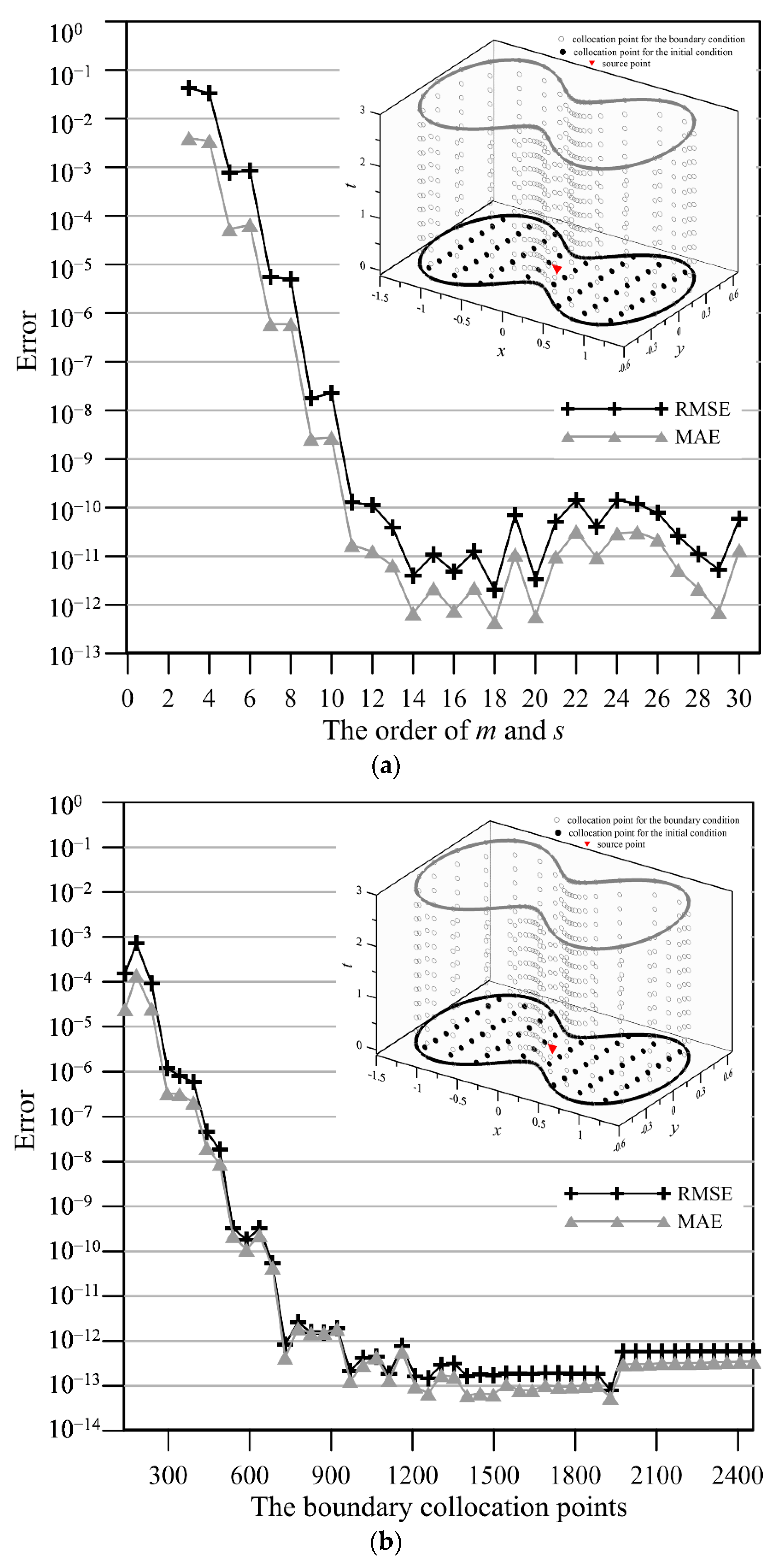
3. Accuracy and Convergence Analysis

A transient groundwater problem in two dimensions is conducted. The shape of irregular geometry is expressed as

$$\partial {\Omega }_t=\left\{(r,\theta ,t)|\begin{array}{l}r=\sqrt{\cos (2\theta )\sqrt{1.1-{\sin }^2(2\theta })},\\ 0\le \theta \le 2\pi ,0\le t\le 3\end{array}\right\}.$$

(22)

The initial data is

$$h=\sin (r\cos \theta )\cos (r\sin \theta ),(r,\theta )\in {\Omega }_t.$$

(23)

The over-specified boundary conditions are applied using the following exact solution.

$$h=e^{-2Dt}\sin (r\cos \theta )\cos (r\sin \theta ),(r,\theta ,t)\in {\Omega }_t.$$

(24)

In this example, the hydraulic diffusivity is 10⁻² and the final elapsed time is 3 s. To validate our approach, a convergence analysis is firstly conducted. The following error is then evaluated

$$\mathrm{RMSE}=\sqrt{\frac{{\displaystyle \sum _{i=1}^{N_I}{(h_E(r_i,{\theta }_i,t_i)-h_N(r_i,{\theta }_i,t_i))}^2}}{N_I}},$$

(25)

$$\mathrm{MAE}=\mathrm{maximum}\left|h_E(r_i,{\theta }_i,t_i)-h_N(r_i,{\theta }_i,t_i)\right|,1\le i\le N_I,$$

(26)

where $h_E(r_i,{\theta }_i,t_i)$ is the exact solution, $h_N(r_i,{\theta }_i,t_i)$ is the numerical approximation, RMSE denotes the root mean square error, MAE denotes the maximum absolute error, and $N_I$ denotes the scattered inner points. Figure 2a shows the error versus the order of the basis functions. It appears that approximations with high accuracy are acquired while the order is superior to 14. The relationship between the absolute error and the number of boundary points is displayed in Figure 2b. Results obtained illustrate that approximations with high accuracy are achieved while the number of boundary points is greater than 900.

4. Numerical Examples

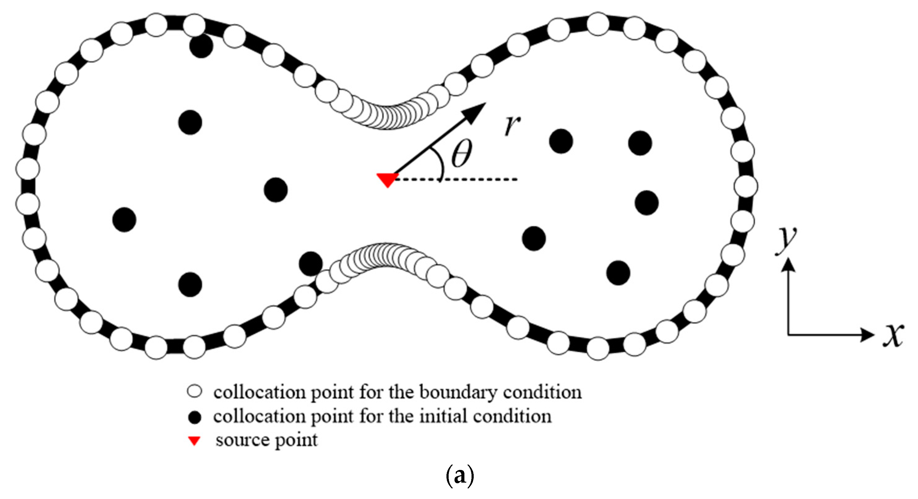
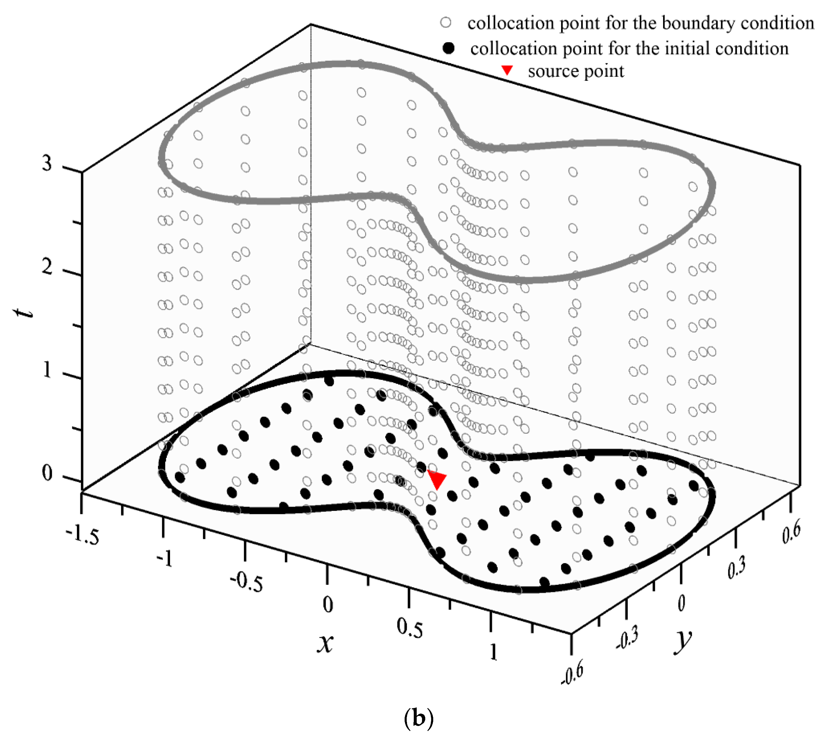
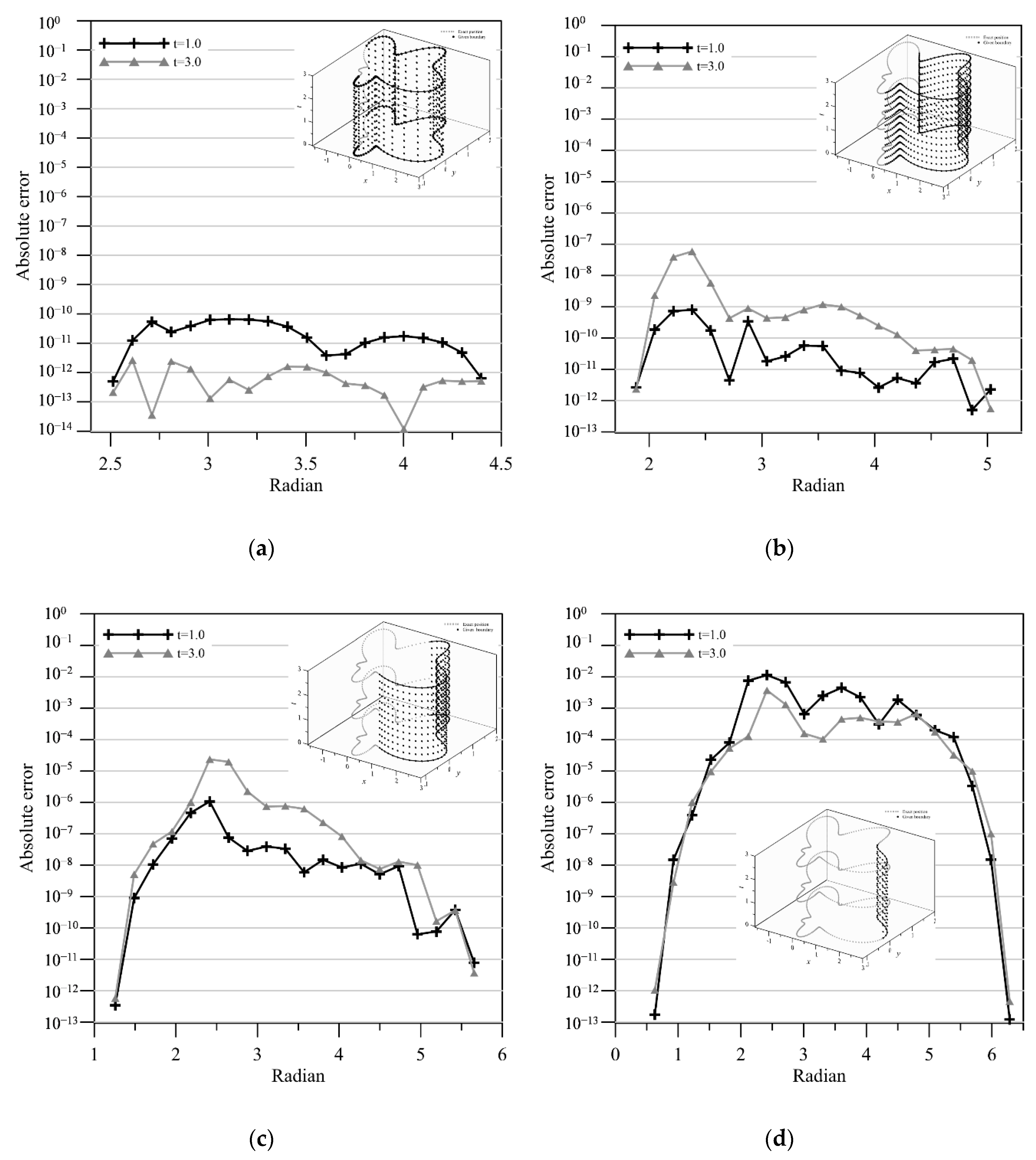
4.1. An Inverse Transient Groundwater Problem—A Cassini-like Boundary

The transient groundwater inverse problem is described as Equation (1). A two-dimensional Cassini-like boundary, as displayed in Figure 3, is defined as follows.

$$\partial {\Omega }_{\mathrm{given}}=\left\{(r,\theta ,t)|\begin{array}{l}r=\sqrt[3]{\cos (3\theta )+\sqrt{2-{\sin }^2(3\theta )}},\\ 0\le \theta \le 1.5\pi ,0\le t\le 3\end{array}\right\}.$$

(27)

From Figure 3, not only the initial data are absent, but part of the boundary information is also not given. The specified boundary data are

$$h=e^{-2Dt}\sin (r\cos \theta )\cos (r\sin \theta ),(r,\theta ,t)\in \partial {\Omega }_{\mathrm{given}},$$

(28)

$$h_n=\frac{\partial h}{\partial n},(r,\theta ,t)\in \partial {\Omega }_{\mathrm{given}}.$$

(29)

The final time is 3 s, and hydraulic diffusivity is 0.1. The number of boundary points and the order of the basis functions are 1173 and 15, respectively. In addition, the parameters including $\delta =0.8$, $v=1.9$, $m=0.1$, and $\epsilon ={10}^{-12}$ are considered in this numerical implementation.

To obtain the recovered boundary data, 240 boundary points are assigned to the recovered boundary positions. To show the stability of our approach, the measured data are polluted by noise, where the noise levels are $s=0.001$, $s=0.01$, and $s=0.1$. Figure 4 depicts the recovered boundary data by adding different noise levels. It seems that the recovered boundary data utilizing our method are consistent with the exact boundary data. However, Figure 4d shows that the discrepancy between numerical and analytical solution (at t = 0.2 s) with $s=0.1$ may be found due to the large noise. Figure 5 displays the absolute error of our method at t = 0.2 s and t = 2.8 s. From Figure 5, the MAE (at t = 2.8 s) with $s=0$, $s=0.001$, $s=0.01$, and $s=0.1$ can reach the order of 10⁻¹⁰, 10⁻⁴, 10⁻³, and 10⁻², respectively.

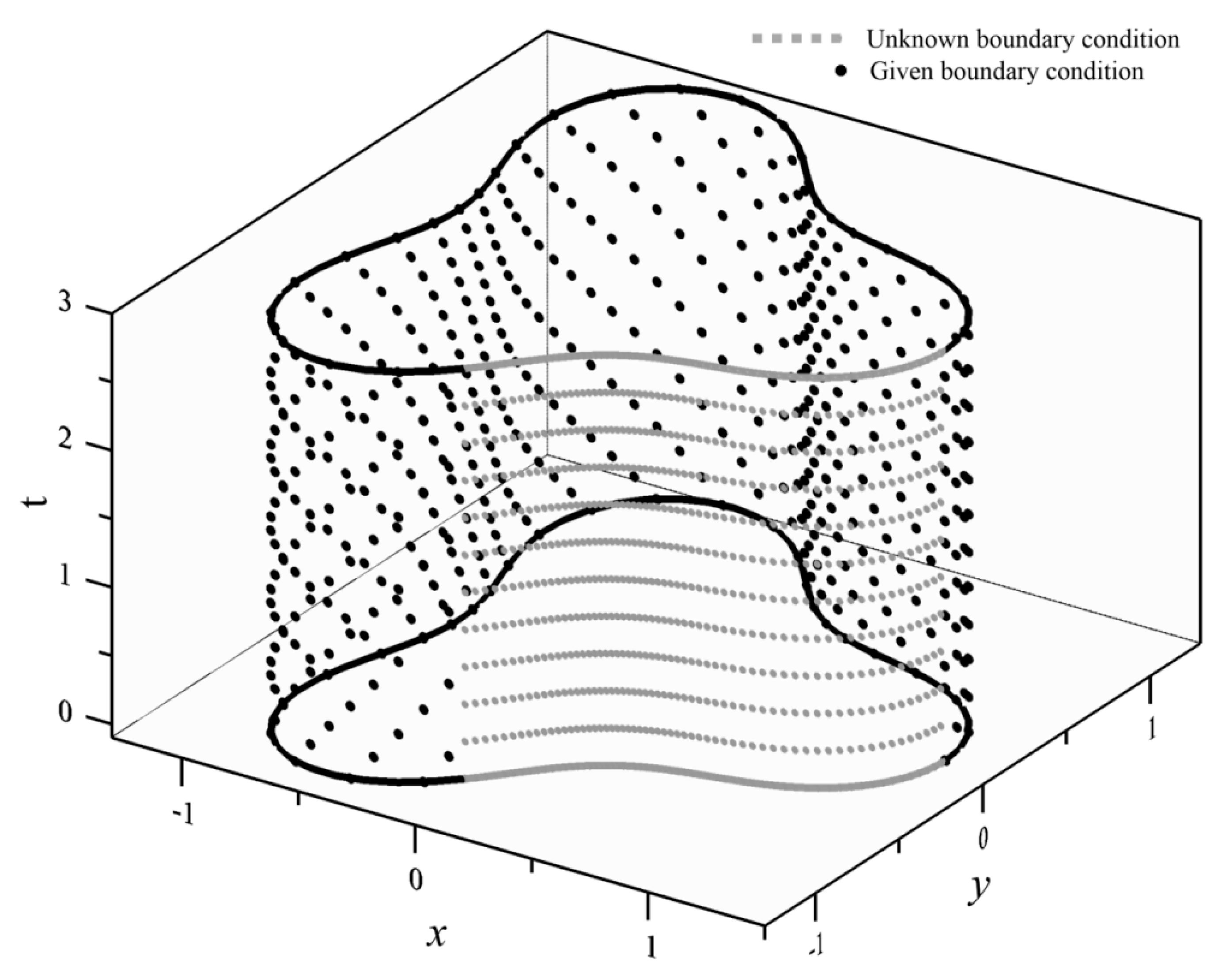
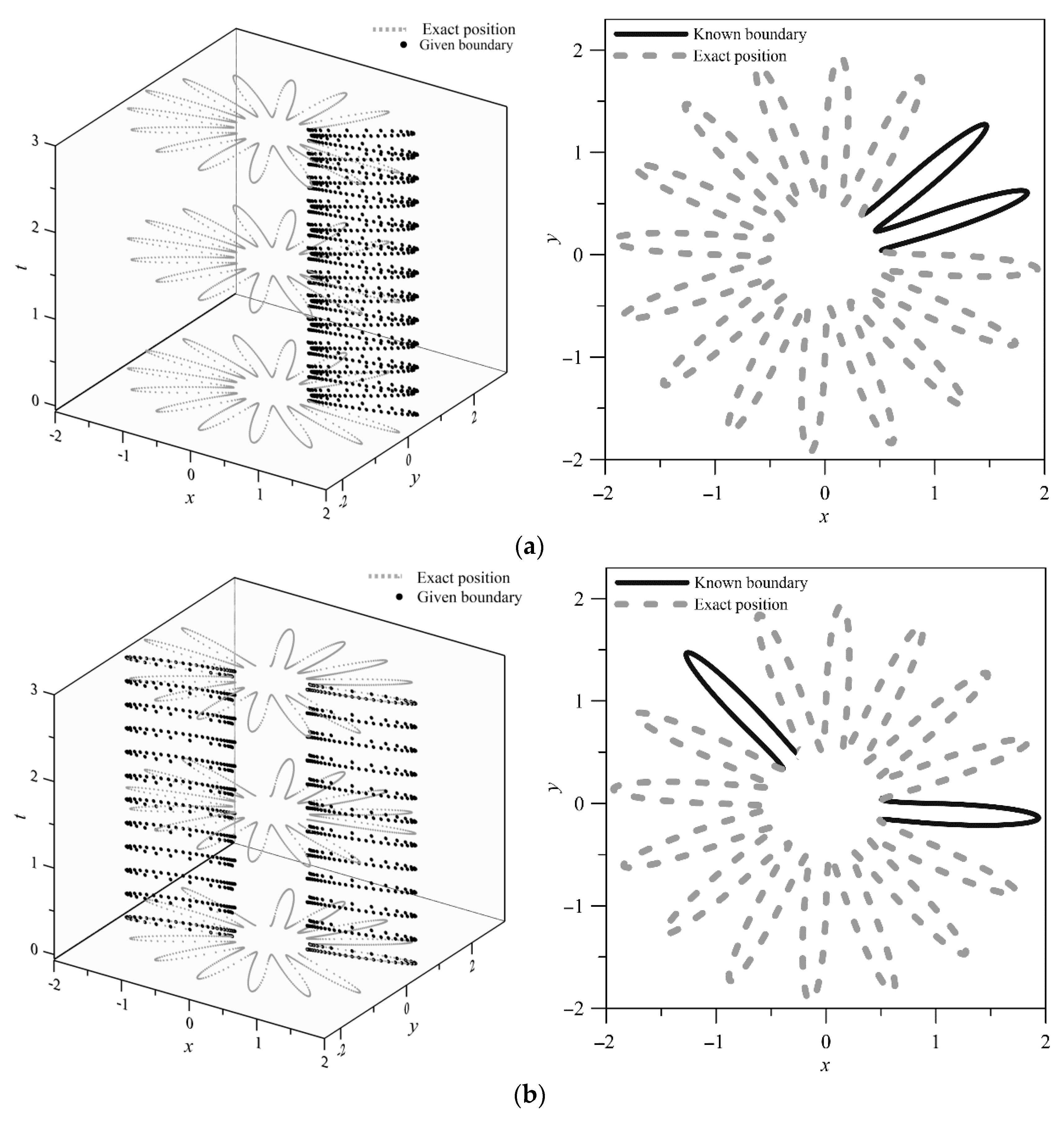
4.2. A Boundary Detection Problem—An Amoeba-like Boundary

The second example is to investigate the effectiveness and stability of the proposed method to solve this boundary detection problem. The transient groundwater inverse problem is described as Equation (1). We consider the given boundary positions defined by Equations (30)–(33) for four different cases in Figure 6.

$$\partial {\Omega }_{\mathrm{given}}=\left\{(r,\theta ,t)|\begin{array}{l}r=e^{\sin (\theta )}{\sin }^2(2\theta )+e^{\cos (\theta )}{\cos }^2(2\theta ),\\ -0.6\pi \le \theta \le 0.8\pi ,0\le t\le 3\end{array}\right\},$$

(30)

$$\partial {\Omega }_{\mathrm{given}}=\left\{(r,\theta ,t)|\begin{array}{l}r=e^{\sin (\theta )}{\sin }^2(2\theta )+e^{\cos (\theta )}{\cos }^2(2\theta ),\\ -0.4\pi \le \theta \le 0.6\pi ,0\le t\le 3\end{array}\right\},$$

(31)

$$\partial {\Omega }_{\mathrm{given}}=\left\{(r,\theta ,t)|\begin{array}{l}r=e^{\sin (\theta )}{\sin }^2(2\theta )+e^{\cos (\theta )}{\cos }^2(2\theta ),\\ -0.2\pi \le \theta \le 0.4\pi ,0\le t\le 3\end{array}\right\},$$

(32)

$$\partial {\Omega }_{\mathrm{given}}=\left\{(r,\theta ,t)|\begin{array}{l}r=e^{\sin (\theta )}{\sin }^2(2\theta )+e^{\cos (\theta )}{\cos }^2(2\theta ),\\ 0\le \theta \le 0.2\pi ,0\le t\le 3\end{array}\right\}.$$

(33)

From Figure 6, not only the initial conditions are inaccessible, but partial boundaries are unspecified. Four different combinations of inaccessible space–time boundaries are conducted, as displayed in Figure 6. In case A, we consider a boundary detection problem, where 70% of the overall space–time boundary positions are given, as depicted in Figure 6a. In cases B, C, and D, not only the initial data but also parts of the space–time boundary positions are inaccessible. The percentage of the given boundary positions in cases B, C, and D is 50%, 30%, and 10%, respectively. As shown in Figure 6b–d, the specified boundary data are given at a partial portion of the space–time boundaries. The specified data are

$$h={(r\cos (\theta ))}^2+{(r\sin (\theta ))}^2+4Dt,(r,\theta ,t)\in \partial {\Omega }_{\mathrm{given}},$$

(34)

$$h_n=\frac{\partial h}{\partial n},(r,\theta ,t)\in \partial {\Omega }_{\mathrm{given}}.$$

(35)

The boundary data on the unknown boundary positions are applied as

$$h={(r_i\cos ({\theta }_i))}^2+{(r_i\sin ({\theta }_i))}^2+4D{t}_i,(r_i,{\theta }_i,t_i)\in \partial {\Omega }_{\mathrm{unknown}}$$

(36)

where $(r_i,{\theta }_i,t_i)$ are the positions of the unknown boundary. In this two–dimensional boundary detection problem, the final elapsed time is 3 s, and the hydraulic diffusivity is 0.1. The number of collocation points and the order of the basis functions to be 960 and 15, respectively. In addition, the parameters including $\delta =0.8$, $v=1.9$, $m=0.1$, and $\epsilon ={10}^{-12}$ are considered in this numerical implementation.

To recover the boundary positions at different times, 60 boundary collocation points are collocated. It seems that unspecified boundary positions can be completely recovered, as shown in Figure 7.

Figure 8 depicts the absolute error of our method at different times. Results show that the MAE without noise for case A to case D are 10⁻¹⁰, 10⁻⁷, 10⁻⁵, and 10⁻², respectively. The accessible data polluted by noise are further considered, where the noise level is s = 0, s = 1, s = 3, s = 5, and s = 10 in case A.

Table 2. Error of the proposed approach for case A.

Noise Level	$\mathit{s} = 0$	$\mathit{s} = 1$	$\mathit{s} = 3$	$\mathit{s} = 5$	$\mathit{s} = 10$
MAE	$6.55\times {10}^{-11}$	$2.62\times {10}^{-2}$	$1.91\times {10}^{-1}$	$2.83\times {10}^{-1}$	$1.05\times {10}^0$
RMSE	$1.98\times {10}^{-11}$	$2.07\times {10}^{-2}$	$5.46\times {10}^{-2}$	$8.88\times {10}^{-2}$	$2.98\times {10}^{-1}$

indicates the error with different noise levels. It appears that inaccessible boundary positions may be recovered even when noises are polluting the specified data.

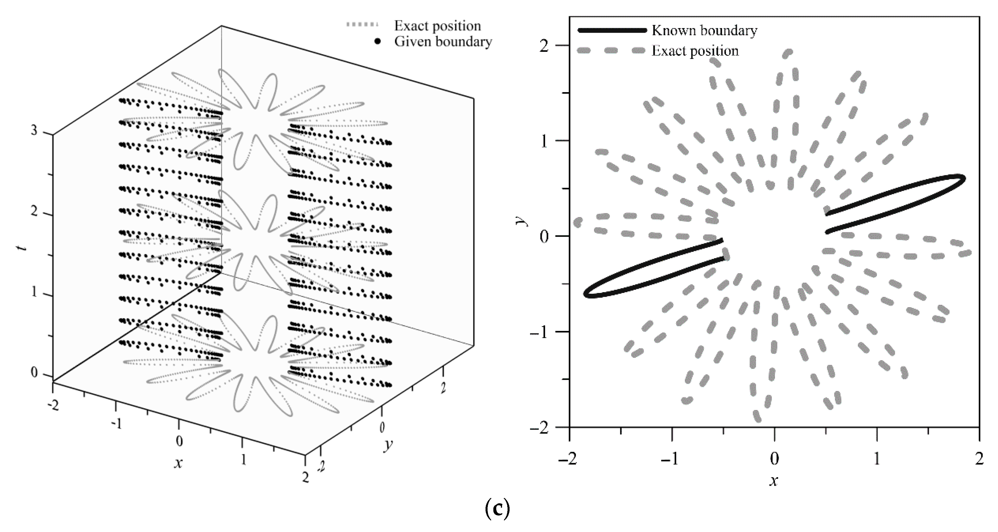
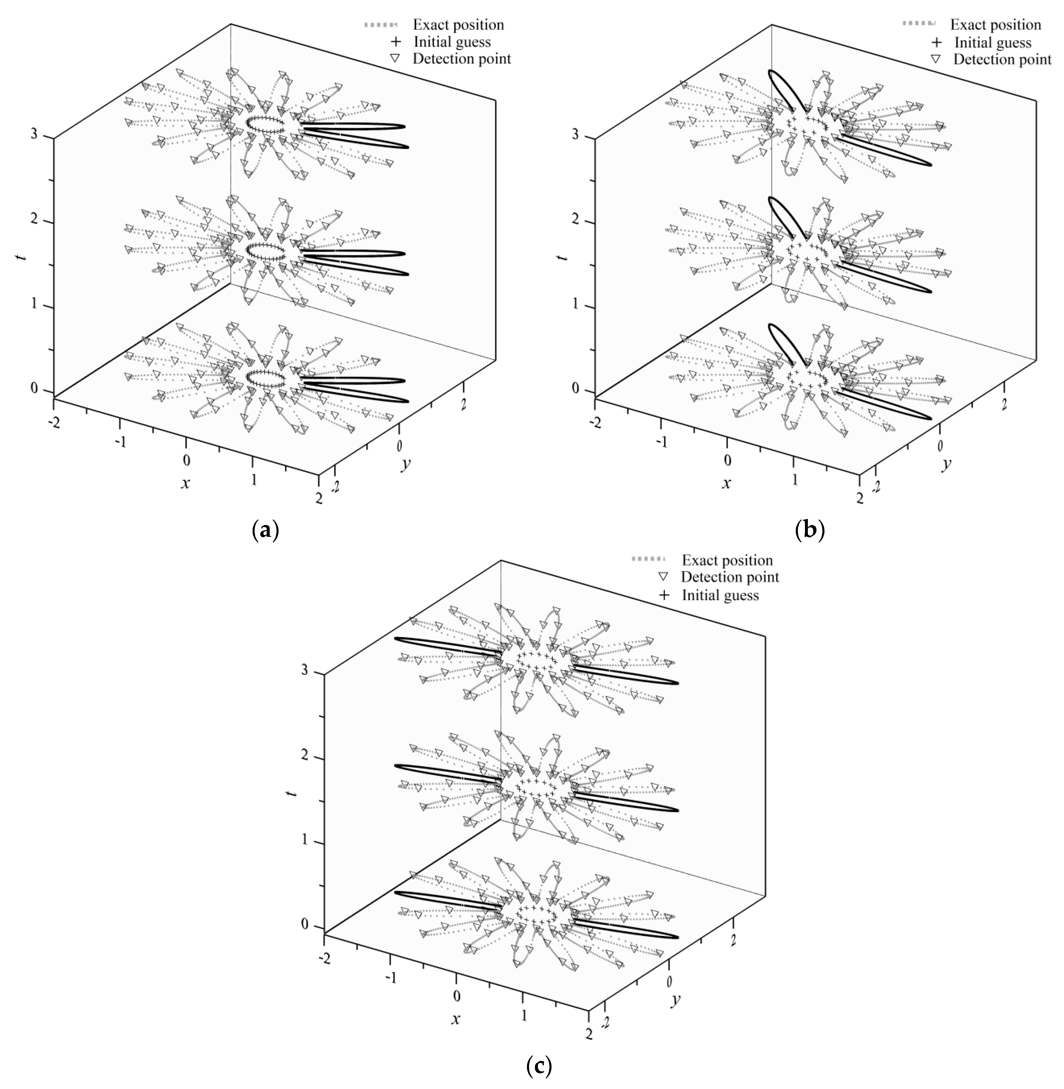
4.3. A Boundary Detection Problem—A Flower-like Boundary

Three cases for the different combinations of unspecified boundary positions are conducted in this problem. For cases 1, 2, and 3 in Figure 9, the specified boundary locations are defined by Equations (37), (38), and (39), respectively.

$$\partial {\Omega }_{\mathrm{given}}=\left\{(r,\theta ,t)|\begin{array}{l}r={\left|\tan (4\theta )\right|}^{\sin (8\theta )},\\ 0.025\pi \le \theta \le 0.275\pi ,0\le t\le 3\end{array}\right\},$$

(37)

$$\partial {\Omega }_{\mathrm{given}}=\left\{(r,\theta ,t)|\begin{array}{l}r={\left|\tan (4\theta )\right|}^{\sin (8\theta )},0\le t\le 3\\ -0.1\pi \le \theta \le 0.025\pi ,0.65\pi \le \theta \le 0.775\pi \end{array}\right\},$$

(38)

$$\partial {\Omega }_{\mathrm{given}}=\left\{(r,\theta ,t)|\begin{array}{l}r={\left|\tan (4\theta )\right|}^{\sin (8\theta )},0\le t\le 3\\ 0.025\pi \le \theta \le 0.15\pi ,1.025\pi \le \theta \le 1.15\pi \end{array}\right\}.$$

(39)

From Equations (37)–(39), it is found that the accessible boundary data are only assigned at 1/8 portion of the space–time boundary.

The specified boundary data are assigned as

$$h=e^{-2Dt}\sin (r\cos (\theta ))\sin (r\sin (\theta )),(r,\theta ,t)\in \partial {\Omega }_{\mathrm{given}},$$

(40)

$$h_n=\frac{\partial h}{\partial n},(r,\theta ,t)\in \partial {\Omega }_{\mathrm{given}}.$$

(41)

The boundary data on the unknown boundary positions are applied.

$$h=e^{-2D{t}_i}\sin (r_i\cos ({\theta }_i))\sin (r_i\sin ({\theta }_i)),(r_i,{\theta }_i,t_i)\in \partial {\Omega }_{\mathrm{unknown}}$$

(42)

In this two-dimensional boundary detection problem, the final elapsed time is 3 s, and the hydraulic diffusivity is 0.1. The number of boundary points and the order of the basis functions are 960 and 15, respectively. In addition, the parameters including $\delta =0.8$, $v=1.9$, $m=0.1$, and $\epsilon ={10}^{-12}$ are considered in this numerical implementation.

To recover the boundary positions at different times, 240 boundary collocation points are collocated. It seems that the inaccessible boundary locations are completely recovered, as displayed in Figure 10. The absolute error of our approach for solving this boundary detection problem is also evaluated. Results obtained demonstrate that the MAE for case 1 to case 3 is 10⁻³, 10⁻⁴, and 10⁻⁵, respectively. It seems that the unknown boundary positions may be completely recovered, even 7/8 portion of the overall space–time boundaries are inaccessible.

5. Conclusions

We present a space–time meshfree method for solving transient groundwater inverse problems in this article. Key findings are described herein.

(1)

For modeling of the two-dimensional transient groundwater inverse problems, an innovative concept, that the collocation points are placed on the space–time boundaries, is presented. Both the initial and boundary data are regarded as boundary conditions on the space–time boundary. Using the space–time collocation, the initial value problem (IVP) for solving the transient groundwater equation is considered to be a problem of the inverse boundary value where the time marching for the IVP can be avoided.

(2)

Previous studies depict that the Trefftz method is limited to linear and stationary problems. This study demonstrates that we solved transient groundwater inverse problems using the space–time meshfree method utilizing Trefftz functions with very high accuracy. The iterative scheme of the FTIM is utilized to deal with the system of nonlinear algebraic equations, which is resulted from spatial discretization of the space–time collocation Trefftz method. The advantages of the proposed meshfree method for solving inverse problems are also presented. Accurate approximations are yielded in which inaccessible boundary may be recovered, even 7/8 portion of the overall space–time boundaries are inaccessible.

(3)

The approximations of the transient groundwater boundary detection problem in two dimensions were developed. The geometric shape of inaccessible parts of the domain remains unknown and is obtained by solving the nonlinear equation formulated from the Trefftz functions and the coefficients. The fictitious time integration method was successfully applied for the solution of the nonlinearity. Highly accurate results for the two-dimensional transient groundwater boundary detection problem were obtained using the proposed space–time meshfree method.

References

1. Azaiez, M.; Ben Abda, A.; Ben Abdallah, J. Revisiting the Dirichlet-to-Neumann solver for data completion and application to some inverse problems. Math. Mech. 2005, 1, 106–121. [Google Scholar]
2. Ling, L.; Takeuchi, T. Boundary control for inverse Cauchy problems of the Laplace equations. CMES-Comp. Model. Eng. Sci. 2008, 29, 45–54. [Google Scholar]
3. Thomas, A.; Majumdar, P.; Eldho, T.I.; Rastogi, A.K. Simulation optimization model for aquifer parameter estimation using coupled meshfree point collocation method and cat swarm optimization. Eng. Anal. Bound. Elem. 2018, 91, 60–72. [Google Scholar] [CrossRef]
4. Fan, C.M.; Chan, H.-F.; Kuo, C.-L.; Yeih, W. Numerical solutions of boundary detection problems using modified collocation Trefftz method and exponentially convergent scalar homotopy algorithm. Eng. Anal. Bound. Elem. 2012, 36, 2–8. [Google Scholar] [CrossRef]
5. Irsa, J.; Zhang, Y. A direct method of parameter estimation for steady state flow in heterogeneous aquifers with unknown boundary conditions. Water Resour. Res. 2012, 48. [Google Scholar] [CrossRef] [Green Version]
6. Ku, C.Y.; Liu, C.-Y.; Xiao, J.-E.; Yeih, W.; Fan, C.-M. A spacetime meshless method for modeling subsurface flow with a transient moving boundary. Water 2019, 11, 2595. [Google Scholar] [CrossRef] [Green Version]
7. Wang, F.; Fan, C.M.; Hua, Q.; Gu, Y. Localized MFS for the inverse Cauchy problems of two-dimensional Laplace and biharmonic equations. Appl. Math. Comput. 2020, 364, 124658. [Google Scholar] [CrossRef]
8. Xi, Q.; Fu, Z.; Wu, W.; Wang, H.; Wang, Y. A novel localized collocation solver based on Trefftz basis for potential-based inverse electromyography. Appl. Math. Comput. 2020, 390, 125604. [Google Scholar] [CrossRef]
9. Ku, C.Y.; Xiao, J.E.; Huang, W.P.; Yeih, W.; Lui, C.-Y. On solving two-dimensional inverse heat conduction problems using the multiple source meshless method. Appl. Sci. 2019, 9, 2629. [Google Scholar] [CrossRef] [Green Version]
10. Li, P.W. Space–time generalized finite difference nonlinear model for solving unsteady Burgers’ equations. Appl. Math. Lett. 2020, 114, 106896. [Google Scholar] [CrossRef]
11. Solyaev, Y.O.; Lurie, S.A. Trefftz collocation method for two-dimensional strain gradient elasticity. Int. J. Numer. Methods Eng. 2020. [Google Scholar] [CrossRef]
12. Zhao, W.; Hon, Y.C.; Stoll, M. Numerical simulations of nonlocal phase-field and hyperbolic nonlocal phase-field models via localized radial basis functions-based pseudo-spectral method (LRBF-PSM). Appl. Math. Comput. 2018, 337, 514–534. [Google Scholar] [CrossRef]
13. Zhang, T.; Li, X. Variational multiscale interpolating element-free Galerkin method for the nonlinear Darcy–Forchheimer model. Comput. Math. Appl. 2020, 79, 363–377. [Google Scholar] [CrossRef]
14. Huybrechs, D.; Olteanu, A.E. An oversampled collocation approach of the wave based method for Helmholtz problems. Wave Motion. 2019, 87, 92–105. [Google Scholar] [CrossRef] [Green Version]
15. Kołodziej, J.A.; Grabski, J.K. Many names of the Trefftz method. Eng. Anal. Bound. Elem. 2018, 96, 169–178. [Google Scholar] [CrossRef]
16. Piltner, R. Some remarks on Trefftz type approximations. Eng. Anal. Bound. Elem. 2019, 101, 102–112. [Google Scholar] [CrossRef]
17. Fu, Z.J.; Yang, L.W.; Zhu, H.Q.; Xu, W.Z. A semi-analytical collocation Trefftz scheme for solving multi-term time fractional diffusion-wave equations. Eng. Anal. Bound. Elem. 2019, 98, 137–146. [Google Scholar] [CrossRef]
18. Trefftz, E. Ein gegenstück zum ritzschen verfahren. In Proceedings of the 2nd International Congress for Applied Mechanics, Zurich, Switzerland, 12–17 September 1926; pp. 131–137. [Google Scholar]
19. Li, Z.C.; Lu, Z.Z.; Hu, H.Y.; Cheng, H.D. Trefftz and Collocation Methods; WIT Press: Southampton, UK, 2008. [Google Scholar]
20. Liu, Y.C.; Fan, C.M.; Yeih, W.; Ku, C.-Y.; Chu, C.-L. Numerical solutions of two-dimensional Laplace and biharmonic equations by the localized Trefftz method. Eng. Anal. Bound. Elem. 2020. [Google Scholar] [CrossRef]
21. Borkowski, M.; Moldovan, I.D. On rank-deficiency in direct Trefftz method for 2D Laplace problems. Eng. Anal. Bound. Elem. 2019, 106, 102–115. [Google Scholar] [CrossRef]
22. Liu, C.S.; Atluri, S.N. A fictitious time integration method (FTIM) for solving mixed complementarity problems with applications to non-linear optimization. CMES-Comp. Model. Eng. Sci. 2008, 34, 155–178. [Google Scholar]
23. Ku, C.Y.; Yeih, W.; Liu, C.S.; Chi, C.C. Applications of the fictitious time integration method using a new time-like function. CMES 2009, 43, 173. [Google Scholar]
Figure 1. The original Euclidean space domain and the space–time collocation scheme: (a) The Euclidean space domain; (b) The space–time scheme.
Water 12 03580 g001aWater 12 03580 g001b
Figure 2. Convergence analysis: (a) The error versus the order; (b) The error versus the boundary points number.
Water 12 03580 g002
Figure 3. The space–time collocation scheme of this study.
Water 12 03580 g003
Figure 4. The computed results: (a) s = 0; (b) s = 0.001; (c) s = 0.01; (d) s = 0.1.
Water 12 03580 g004
Figure 5. The absolute error: (a) s = 0; (b) s = 0.001; (c) s = 0.01; (d) s = 0.1.
Water 12 03580 g005
Figure 6. Four cases for missing space–time boundary conditions: (a) case A; (b) case B; (c) case C; (d) case D.
Water 12 03580 g006
Figure 7. Recovered boundary positions at different times: (a) case A; (b) case B; (c) case C; (d) case D.
Water 12 03580 g007
Figure 8. Absolute error of the results at different times: (a) case A; (b) case B; (c) case C; (d) case D.
Water 12 03580 g008
Figure 9. The collocation scheme: (a) case 1; (b) case 2; (c) case 3.
Water 12 03580 g009aWater 12 03580 g009b
Figure 10. Recovered boundary positions at different times: (a) case 1; (b) case 2; (c) case 3.
Water 12 03580 g010