The Response of Lateral Flow to Peak River Discharge in a Macrotidal Estuary


1
Key Laboratory of Physical Oceanography, Ministry of Education, Ocean University of China, Qingdao 266100, China
2
Pilot National Laboratory for Marine Science and Technology, Qingdao 266237, China
3
College of Oceanic and Atmospheric Sciences, Ocean University of China, Qingdao 266100, China
*
Author to whom correspondence should be addressed.
Water 2020, 12(12), 3571; https://doi.org/10.3390/w12123571
Submission received: 22 November 2020
/
Revised: 13 December 2020
/
Accepted: 15 December 2020
/
Published: 19 December 2020
(This article belongs to the Special Issue Hydrodynamics in Estuaries and Coast: Analysis and Modeling)
Abstract
:The Ou River, a medium-sized river in southeastern China, is selected to study the lateral flow response to rapidly varied river discharge, i.e., peak river discharge (PRD). A three-dimensional model based on the Finite-Volume Community Ocean Model is validated by in situ measurements from 15 June to 16 July 2005. PRD, which considers the extra buoyancy and longitudinal momentum in a short time, rebuilds the stratification and lateral flow. PRD, compared with low-discharge, generally makes stratification stronger and lateral flow weaker. PRD mainly rebuilds lateral flow by changing lateral advection, lateral Coriolis, and lateral-barotropic pressure gradient terms. After PRD, the salinity recovery time is longer than that of the flow because the impact on buoyancy lasts longer than that on longitudinal flow. Longitudinal flow is mostly affected by the momentum transferred during PRD; therefore, the recovery time is close to the flooding duration. However, the lateral flow is affected by the buoyancy, and its recovery time is generally longer than the flooding duration. The lateral flow recovery time depends on transect width, flow velocity and the variation caused by PRD. PRD occurs widely in global small-/medium-sized river estuaries, and the result of this work can be extended to other estuaries.
1. Introduction
River discharge plays a crucial role in estuarine circulation and material transport [1]. River discharge has been studied in many large river estuaries, such as the Amazon River Estuary [2,3], the Nile River Estuary [4], the Mississippi River Estuary [5,6], and the Yangtze River Estuary [7,8,9]. Due to a lack of connected lakes and tributaries (small drainage basins) acting as sponges, the fluvial flow of small-/medium-sized rivers is likely to form peak river discharge (PRD), i.e., a rapidly varied large-volume flux during a short period under natural conditions (e.g., heavy rainfall or snowmelt) or anthropogenic conditions (e.g., sluice floodwater) [10]. This discharge is different from the steadily increased discharge that occurs during rainy seasons in large rivers (hereafter known as steady flooding) [10]. For example, the maximum discharge of the Amazon River is approximately twice as high as its average river discharge; however, the maximum discharge of small-/medium-sized rivers can be several orders greater than the average discharge with extremely rapid variation [11]. However, according to Milliman and Syvitski [12], the sediment flux from small-/medium-sized rivers has been significantly underestimated, which is also essential to marine geomorphology evolution [13] and biogeochemical processes [14], such as the Trinity River in North America [15], the Tiber River in Europe [16], and the Sepik River in Oceania [17]. In the context of increasing global warming-induced inundation risks [18] and increasing terrestrial sediment sequestration by growing reservoirs [19] in the upstream areas of large rivers, studies on PRD, which is more likely to occur in small-/medium-sized river estuaries, have become important.
Flooding can affect estuarine dynamics, which has been reported in previous studies; however, most of these studies focused on steady flooding rather than PRD [20,21,22]. Based on a theoretical model, MacCready [20,21] explored the impact of steady flooding on salinity and the recovery time for salinity to reach a quasi-steady state after steady flooding in an idealized channel. Hetland and Geyer [22] concluded that the ratio of salt-wedge length to average river-flow velocity was positively correlated with the salinity recovery time. Using numerical modeling in a PRD river estuary with a small tidal range (<0.5 m), Rayson et al. [15] found that a lower PRD corresponds to a shorter salinity recovery time.
Furthermore, runoff imports buoyancy and along-channel momentum into waters; the former can change the stratification structure [23], and the latter can generally enhance seaward flow and may affect lateral circulation [24]. Based on an idealized straight lateral-symmetrical flat-bottom channel, lateral flow has been explored in several studies [25,26,27,28,29,30,31]. The differential advection, stratification, diffusive boundary layer mixing, and Earth’s rotation are the key factors that generate lateral flow when ignoring the curved channel effect. Additionally, wind can import momentum through surface shear stress and drive lateral flow [28,32,33,34]. Chant [35] found that the strengths of lateral flows during PRD were appreciably weaker than those during dry conditions in the Hudson River Estuary based on a 301-day acoustic Doppler current profiler mooring.
It is essential to study lateral flow as it is important in estuarine circulation process [36,37,38,39,40], lateral sediment transport, estuarine turbidity maximum, and estuarine morphology evolution [26,41,42]. However, the response of lateral flow to a PRD has been less documented in previous studies. The Ou River in China, which has a drainage basin area of ~1.80 × 10⁴ km2 [43], is categorized as a medium-sized river [12,44] and frequently suffers PRD from spring to summer. Here, it is used as a case study to explore the response of lateral flow to a PRD. The remainder of this paper is structured as follows. In Section 2, the study area, the numerical model, and numerical experiments are introduced. In Section 3, the model results under different numerical experiments are described. The effects of PRD on estuarine lateral flow are discussed in Section 4, and conclusions are summarized in Section 5.
2. Study Area and Methodology
2.1. Study Area and Observations
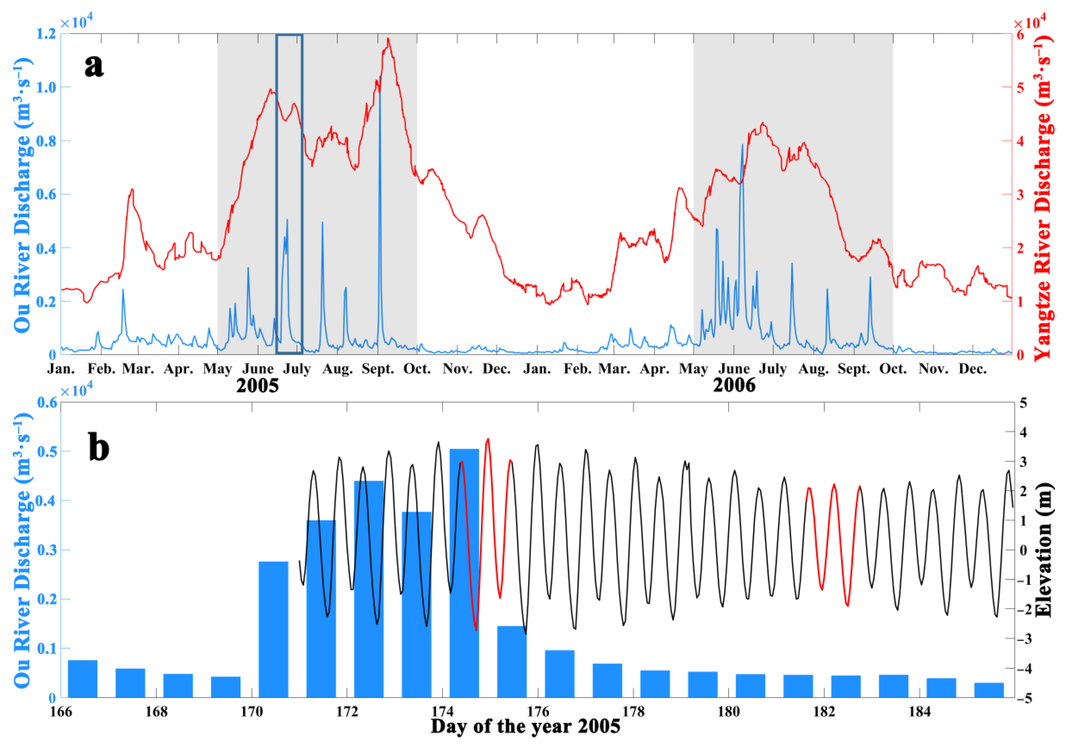
The Ou River (OR), which has a humid subtropical climate, flows 388 km to reach the East China Sea (ECS), mainly through the Huang-Da-Ao Passage (HDAP, Figure 1). The annual discharge of the river is 1.39 × 10¹⁰ m3, which is approximately 1.6% of that of the Yangtze River [45,46], located approximately 400 km north of the OR. However, the OR discharge varies quickly in a short time during the plum-rainy/typhoon season, which is different from that of the Yangtze River (Figure 2a). The OR Estuary (ORE) is tide dominated, and the largest tidal range and the smallest tidal range are 7.21 m and 1.14 m at the Huang-Hua tidal station (HH in Figure 1), respectively, indicating a macrotidal regime [47].
The ORE is split into the North and South Channels by Ling-Kun Island (LKI). To meet the demand of land use by socioeconomic development, a submerged dike (South Channel Submerged Dike, SCSD) was built in 1979 in the South Channel to silt the South Channel and naturally and gradually form land. The North Channel, as a main channel, is further divided into the northeastward Sha-Tou Passage (STP) and the Middle Passage (MP); it stretches along the North Submerged Dike (NSD), Ling-Ni Dike (LND), and several islands, including Da-Men Island (DMI), Ni-Yu Island (NYI) and Zhuang-Yuan-Ao Island (ZYAI) (see Figure 1b for details).
Fieldwork was carried out in the ORE in the plum-rainy/typhoon season of 2005 (Figure 1). Tidal elevations (blue triangles in Figure 1) were recorded hourly at three long-term tidal stations (HH, WXT, and ZYA) and several short-term tidal gauges obtained by Temperature Depths (Compact-TDs). Compact-TDs were set to work in a burst mode with a rate of 1 Hz, which records 60 samples within one burst for each hour, and the burst-averaged data was used as the hourly record. Meanwhile, electromagnetic current meters (ECMs) and Conductivity Temperature Depths (CTDs) were used to record the current velocity and salinity (red stars in Figure 1) during the spring tide from 09:00 23 June to 12:00 24 June (UTC +0800, day of the year 174.38–175.50) and the neap tide from 15:00 30 June to 19:00 1 July 2005 (UTC +0800, day of the year 181.63–182.79) with one-hour intervals. ECMs and CTDs were also set to work at a sampling rate of 1 Hz, and for each hour they were deployed to measure the profiles of current, temperature, and salinity. The daily average river discharge was obtained from the Xuren hydrologic station in the OR and the Shizhu hydrologic station in the Nanxi River (NR) (red triangles in Figure 1d). A PRD event was captured during the field measurements (Figure 2b).
Two transects along the MP (the red cross-channel lines in Figure 1b,c) are selected for flow and stratification analysis. Transect I is near the observed stations. Meanwhile, Transects I and II represent two typical bathymetric features in the ORE: Transect I is located in the narrower channel with a shallow sill along the channel, and Transect II has a wider width and a submerged dike (NSD), approximately 0.6 m below the mean sea level, on the north.
The observed longitudinal flow, lateral flow and salinity near Transect I were considered at four different tidal stages in Figure 3. Note that all the cross-channel plots in this study are landward looking, and the local horizontal coordinates of transects are defined to be positive seaward (perpendicular to the transects downstream, x-axis) and positive to the right (landward looking, northward along the transects, y-axis). Figure 3a,i illustrate that the ebb flow and freshwater began from the south in the North Channel, and longitudinal flow reached the maximum in the Deep Navigation Channel (DNC, labeled in Figure 3j) at maximum ebb tide (Figure 3c). Upstream longitudinal flow also began from the south at low water slack (Figure 3e), and the magnitude was dependent on the bathymetry at maximum flood tide (Figure 3g). The lateral flow seemed discontinuous because the observation stations were not strictly in a straight line (Figure 3b,d,f,h). At high water slack, the southward flow was mostly located at the shoal bottom and the DNC surface (labeled in Figure 3j), and the rest was mostly northward (Figure 3b). Lateral flow was mostly southward at maximum ebb tide, and the water flowed northward near the south head of the transect and the DNC bottom (Figure 3d). At low water slack, the southward flow covered the shoal surface and the DNC, and the other part was northward flow (Figure 3f). Lateral flow was mostly northward at maximum flood tide, and the water near both the north and south heads of the transect flowed southward, although southward flow was weak at the DNC (less than 0.1 m·s−1) (Figure 3h). As the salt wedge was pushed downstream by flooding at some moment during the fieldwork, these observations cannot reveal the intratidal salinity variation and show only the salinity structure at high water slack (Figure 3i).
2.2. Model Configuration
The numerical model used here is the three-dimensional unstructured grid primitive equation Finite-Volume Community Ocean Model (FVCOM) [48,49]. Irregular triangular grids employed by the FVCOM are suitable for fitting the complex coastlines in the ORE. Some of the coastline and bathymetry data (mainly at the channels) were measured in situ in May 2005, and the other datasets were obtained from the official marine charts published by the Maritime Safety Administration of China in 2005. The resolution of the topography and bathymetry varies from 60 m at the channels to about 5 km in the open ocean. The baroclinic model has a horizontal resolution varies from 100 m in the North Channel and MP to 2–5 km in the open ocean (Figure 1d), and 18 uniformed sigma layers in the vertical direction. The daily average river discharge at the Xuren and Shizhu hydrologic stations was used as the OR and NR discharges (red triangles in Figure 1d). Eight primary tidal constituents (M2, S2, N2, K2, K1, O1, P1, and Q1) were obtained from the NAO.99b tidal prediction system (http://www.miz.nao.ac.jp/staffs/nao99/index_En.html), and three quarter-diurnal tides (M4, MS4, and MN4) were derived from an ECS numerical model [50]. The water level calculated by the above tidal constituents was used as the open boundary forcing (the red curves in Figure 1a,d indicate open boundary). Sea surface wind (hourly and 0.312° × 0.312° grid) was obtained from NCEP Climate Forecast System Reanalysis (CFSR) Selected Hourly Time-Series Products (http://rda.ucar.edu/datasets/ds093.1/). The initial salinity and monthly average salinity at the open boundary were derived from the same ECS model [50]. The summer-observed surface-bottom temperature difference is less than 1 °C in the ORE and has less of an effect on the variation in density than salinity [51]. Thus, the numerical model was simplified with a constant temperature (20 °C). The model was initiated with zero water level and velocity and was first run for 120 days with a fixed river discharge, including both OR and NR (the daily average on 1 June 2005) and the open boundary salinity (the monthly average in June 2005) to reach a quasi-equilibrium state. Then, the model was run with daily average river discharge for another 45 days from 1 June to 15 July 2005, and the results from the last 35 days were analyzed. The wind wave was nonsignificant in the ORE due to the shelter effect of the island [52] and thus was not considered in this study. This case was marked as the Control Run (Run 0).
2.3. Validation
To validate the numerical model, the skill score (SS) is used here, which is the ratio of the root mean square error (RMSE) normalized by the standard deviation of the observation [53]:
where is the variable being evaluated and is the temporal average. Referring to previous studies [8,54], an SS greater than 0.65 can be acknowledged as an excellent simulation, and an SS less than 0.20 is considered poor. The SS indicates the accuracy of the model result. Furthermore, the correlation coefficient (CC) between the model result and the observation was used to quantify the variation trend:
The simulated tidal elevation is compared with the observations at 14 stations in the model domain. The SSs and CCs at each station are given in Table 1. All the values exceed 0.90, indicating that the model can well reproduce the tidal elevation. Comparisons between the observed and simulated water levels at the three long-term tidal stations are shown in Figure 4a–c. During spring tide, most of the SSs for the current velocity are over 0.65, and the CCs are over 0.90 (Table 2). During neap tide, the SSs and CCs are also excellent at most stations, except those in the nonmainstream direction. Taking No. 8 station as an example, visual comparisons between the simulated and observed current velocity/direction during spring tide and neap tide are shown in Figure 4d–g.
A comparison of SSs and CCs between the simulated and observed salinities is summarized in Table 3, which indicates that the model could reproduce the salinity variation. Note that an episode of peak river discharge occurred during the observed spring tide, and the daily average discharge measurement could not accurately reproduce the hourly salt-wedge changes, which has a greater impact on the surface salinity simulation than the bottom (Table 3). Taking No. 8 station as an example, visual comparisons between the simulated and observed salinities during spring tide and neap tide are shown in Figure 5. Overall, this numerical model is able to describe the hydrodynamics in the ORE.
2.4. Experimental Design
Based on the ORE model, several experiments are designed to study the response of the lateral flow to a rapid-change discharge during spring tide, which are summarized in Table 4. The daily average river discharge from 1950 to 2008 at the Xuren hydrologic station shows that the duration of a PRD event is usually less than 48 h in the ORE [46]. Thus, the flooding duration is set to 48 h in this study. In contrast to Run 0, wind and NR are ignored in the other cases to focus on the PRD. The OR discharge was given a PRD type with a peak discharge of 5000 m3·s−1 in Run 1 (the solid blue line with squares in Figure 6a), which represents the PRD that occurred during the observation. Run 2 represents a low-discharge condition with 500 m3·s−1 (the solid blue line in Figure 6a), referring to the multiyear average value of 442 m3·s−1 [46]. The maximum PRD of 23,000 m3·s−1 was recorded in July 1952 [46]; however, the maximum discharge from 2005 to 2015 was only 10,900 m3·s−1, which was recorded in August 2014. Therefore, from Runs 3 to 13, the peak discharge is set to increase from 2500 to 15,000 m3·s−1 with 1250 m3·s−1 intervals to examine the impact of discharge volume on estuarine circulation.
3. Results
3.1. Salinity and Stratification
Without a loss of generality, a typical ebb–flood cycle during spring tide (the first ebb–flood cycle in Figure 6a shows as a red line) is described in this section to show how the PRD changes the stratification in the ORE. Under the low-discharge condition (Run 2), the tidally averaged salinity ranges from 16 psu in Transect II to 8 psu in Transect I. The ebb/flood tide average salinity along the section (purple line in Figure 1b along the DNC) is shown in Figure 6b–e (black lines). The isolines are distributed asymmetrically between the ebb (Figure 6b) and flood (Figure 6c) tides at the DNC under the low-discharge condition (Run 2), indicating difference in mixing between ebb and flood tides; the ebb–tidal-averaged isolines are tilted more than the flood–tidal-averaged isolines, which are nearly vertical in the lower layer. In Run 1, the ebb–tidal-averaged isolines become more tilted (Figure 6d), and the flood–tidal-averaged isolines remain vertical in the lower layer (Figure 6e). Regarding the surface layer, the isolines become more tilted after PRD (Figure 6e), indicating that the PRD can enhance only the stratification on ebb tides and the surface layer (above −4 m) on flood tides. The lower layer on flood tides is still well-mixed even under PRD.
The structure of salinity shows distinctive patterns between two cross-sections, and the PRD changes Transect I more than Transect II. Figure 7 shows the salinity structure in Transects I and II in Runs 1 and 2 at four different tidal stages. For Transect I, under the low-discharge condition (Run 2), the freshwater first presents on the shoal water surface at the beginning of the ebb tide (Figure 7a) and then occupies the entire transect until the maximum ebb tide, while the DNC surface has significant stratification (tilted isolines) (Figure 7b). At low water slack, saltwater intrudes from the shoal bottom (Figure 7c). The intratidal variation in salinity indicates a significant difference in mixing between ebb and flood tides, and the transect is well-mixed at maximum flood tide (Figure 7d). In Run 1, the structure of Transect I salinity has a similar pattern as that in Run 2 at four different tidal stages, but with a smaller magnitude (Figure 7e–h). For Transect II, the saltiest water is mostly located on the part near the north head under the low-discharge condition (Run 2). The freshwater first presents on two heads of the transect surface at high water slack (Figure 7i). At maximum ebb tide, the isolines are mostly vertical, indicating that stratification is not significant, and the saltiest water is mostly located on the north head of the transect (Figure 7j). During flood tide, the saltwater intrudes from two heads of the transect bottom at low water slack (Figure 7k), the water column is well-mixed, and the saltiest water is mostly located on the north head of the transect at maximum flood tide (Figure 7l). In Run 1, the structure of Transect II salinity has a similar pattern as that in Run 2 at four different tidal stages but with a smaller magnitude (Figure 7m–p). For Transect I, the transect-averaged salinity is between 2.2–16.4 psu in Run 2 and between 0.6–15.7 psu in Run 1, and the root mean square (RMS) of the difference between Runs 1 and 2 (Run 1 minus Run 2) is 2.6 psu during the ebb–flood cycle. For Transect II, the transect-averaged salinity ranges between 10.7–23.7 psu in Run 2 and ranges between 8.6–23.5 psu in Run 1, and the RMS of the difference between these two runs is 1.6 psu during the ebb–flood cycle, indicating that PRD has a larger impact on Transect I than on Transect II.
3.2. Lateral Flow
Figure 8a–h show the lateral flow structure in Transect I at four different tidal stages under the low-discharge condition (Run 2) (Figure 8a–d) and the difference between Runs 1 and 2 (Run 1 minus Run 2) or PRD-driven lateral flow (Figure 8e–h) at four different tidal stages. Under the low-discharge condition (Run 2), as a single-channel transect (Transect I), the lateral flow shows that the northward flow is located in the upper layer of the shoal and that the lower layer of the DNC and the southward flow cover the lower layer of the shoal and the upper layer of the DNC at high water slack (Figure 8a); the lateral flow is mostly southward at maximum ebb tide (Figure 8b). At low water slack, the lateral flow is southward in the upper layer and northward in the lower layer at the shoal; at the DNC, the lateral flow is mostly northward (Figure 8c). The Transect I shallow sill is a barrier to saltwater cross-channel transport by northward near-bottom lateral flow at low water slack; as a result, the water column is almost well-mixed, and lateral flow is mostly northward at the DNC. At maximum flood tide, lateral flow is mostly northward (Figure 8d). For the difference between Runs 1 and 2 (Run 1 minus Run 2), the pattern of PRD-driven flow is mostly opposite to but smaller than that under the low-discharge condition (Run 2) at high water slack (Figure 8e), and it is mostly southward at maximum ebb tide (Figure 8f). During flood tide, the pattern of PRD-driven flow is also opposite to but smaller than that under the low-discharge condition (Run 2) at low water slack (Figure 8g), and it is mostly southward at maximum flood tide (Figure 8h).
Figure 8i–p show the lateral flow structure in Transect II at four different tidal stages under the low-discharge condition (Run 2) (Figure 8i–l) and the difference between Runs 1 and 2 (Run 1 minus Run 2) or PRD-driven lateral flow (Figure 8m–p) at four different tidal stages. Under the low-discharge condition (Run 2), for a partially blocked transect (Transect II) by submerged dike NSD, lateral flow has a two-layer structure, with northward flow in the upper and southward flow in the lower at high water slack (Figure 8i); lateral flow is mostly northward at maximum ebb tide (Figure 8j). During flood tide, the lateral flow is southward in the upper layer of the southern part and the lower layer of the northern part, and northward flow covers the lower layer of the southern part and the upper layer of the northern part at high water slack in Transect II (Figure 8k), and it is mostly southward at maximum flood tide (Figure 8l). This lateral flow structure at high/low water slack has also been reported in studying the influence of submerged dikes in the Yangtze River Estuary by Chen et al. [55]. The Run 1 PRD-driven lateral flow magnitude is mostly less than 0.05 m·s−1 at four different tidal stages in Transect II. For the difference between Runs 1 and 2 (Run 1 minus Run 2), PRD-driven lateral flow is mostly southward in the upper layer (above −3 m) and is mostly northward in the lower layer at high water slack (Figure 8m). At maximum ebb tide, PRD-driven lateral flow is mostly northward, and small magnitude (<0.01 m·s−1) southward flows are located on the surface of two transect heads (Figure 8n). PRD-driven lateral flow is southward on the near south transect head surface, and the rest is northward at low water slack (Figure 8o); it is mostly northward, and near the two heads, the bottom of the transect is southward at maximum flood tide (Figure 8p).
PRD effect is asymmetric between the discharge rising and falling processes. Figure 9a,b show the difference (color) of the transect-averaged lateral flow between each PRD run and Run 2 (each run minus Run 2) in Transects I and II, which indicate PRD-driven lateral flow. For Transect I, the lateral flow is mostly southward and less than 0.07 m·s−1 in magnitude (Figure 9a). The flooding effect on lateral flow is asymmetric between the discharge rising and falling processes: the maximum speed during the discharge rising process (0.07 m·s−1) is slightly larger than that during the discharge falling process (0.06 m·s−1) in Transect I (Figure 9b). For Transect II, the lateral flow is mostly northward, and the maximum speed during the discharge falling process (0.08 m·s−1) is larger than that during the discharge rising process (0.07 m·s−1) (Figure 9b).
4. Discussion
4.1. Momentum Balance Analysis
Considering a three-dimensional domain, the lateral Reynolds-averaged momentum difference equation [48] is given as follows:
where Δ indicates the difference between PRD and low-discharge conditions, (u, v) are the along- and cross-channel velocities, respectively, w is the vertical velocity, f is the Coriolis parameter, Pt is the barotropic pressure, Pc is the baroclinic pressure, Am is the horizontal diffusion coefficient, Kv is the vertical eddy viscosity coefficient, x and y are orthogonal in the along- and cross-channel directions, respectively, and z is the vertical axis in the Cartesian coordinate system. In the lateral dynamics equation (Equation (3)), the difference of the lateral advection term (−Δuvx) and the difference of the lateral Coriolis term (−Δfu) are directly affected by the longitudinal flow, and these two terms together are referred to as the longitudinal flow-related term, where the subscript (x, y, z, t) indicates the partial derivation. PRD drives seaward longitudinal flow and changes the longitudinal flow-related term, and buoyancy taken by PRD also modifies the lateral-baroclinic-pressure-gradient (ΔPcy); as a result, lateral acceleration changes with them, and the changed lateral flow further alters the remaining terms on the right-hand side of Equation (3). Table 5 shows each transect-averaged lateral momentum term in Runs 1 and 2 after the tidal average, which indicates a PRD effect on lateral momentum; the RMS of the lateral momentum change distribution after the tidal average in the transect is also listed in Table 5 to facilitate the comparison of different term changes in magnitude between Runs 1 and 2. During PRD, compared to Run 2, the lateral acceleration in Transect I decreases from 1.39 × 10⁻⁶ m·s−2 to 0.84 × 10⁻⁶ m·s−2 and that in Transect II increases from −0.69 × 10⁻⁶ m·s−2 to −0.66 × 10⁻⁶ m·s−2 (Table 5). The RMS of lateral acceleration in Transect I (1.84 × 10⁻⁶ m·s−2) is smaller than that in Transect II (7.99 × 10⁻⁶ m·s−2), so the impact of PRD on lateral acceleration in Transect II is larger than that in Transect I (Table 5). The lateral flow in Runs 1 and 2 is controlled by the balance between the longitudinal flow-related term (−uvx−fu), the lateral-barotropic-pressure-gradient term (Pty), and the lateral-baroclinic-pressure-gradient (Pcy) term (Table 5). In Transect I, the difference of the longitudinal flow-related term −Δ(uvx+fu), with the RMS of 14.06 × 10⁻⁶ m·s−2, and the difference in the lateral-barotropic-pressure-gradient (ΔPty), with the RMS of 12.27 × 10⁻⁶ m·s−2, are two of the most significant terms affected by PRD; the RMS of the remaining terms is less than 10 × 10−6 m·s−2 (Table 5). In Transect II, the three terms most significantly affected by PRD are the longitudinal flow-related term −Δ(uvx + fu), with the RMS of 12.33 × 10⁻⁶ m·s−2, the lateral-barotropic-pressure-gradient (ΔPty), with the RMS of 17.16 × 10⁻⁶ m·s−2, and the lateral-baroclinic-pressure-gradient (ΔPcy), with the RMS of 12.84 × 10⁻⁶ m·s−2 (Table 5).
4.2. Recovery Time
In this study, taking the low-discharge salinity as a reference, the salinity recovery time is defined in a subtidal manner as the duration from a decrease to 10% to when the salinity increases back to 90% of the reference value. Additionally, taking the subtidal flow under the low-discharge condition (Run 2) as a reference, the recovery time of flow is defined as the duration from when the flow increases to 10% of the largest difference from the reference to when it falls back to 10% of the difference. The transect averaged subtidal salinity and flow are calculated using a 34 h low-pass filter to avoid the tidal signals disturbance [50]. Figure 10a–f show the changes in transect averaged subtidal salinity, subtidal longitudinal flow and subtidal lateral flow after the beginning of PRD; the numbers represent the recovery time and correspond to the line color. The PRD pushes the salt wedge seaward, and the salinity drops; subtidal salinity even becomes 0 during the high discharge period under a large PRD condition (for example, red line in Figure 10a); subsequently, the saltwater intrudes the estuary again, and the salinity rebounds. Different transects have different recovery times under the same PRD. In Run 1, the salinity recovery time shortens downstream from 204.0 h in Transect I to 103.3 h in Transect II (blue lines in Figure 10a,b). The recovery time increases as the peak discharge rises (Table 6), and in Run 13, the time extends to 303.5 h in Transect I and 172.5 h in Transect II (red lines in Figure 10a,b). In particular, the salinity recovery time in Transect I slows down significantly as the peak discharge rises when the minimum salinity is 0 during PRD (Runs 10–13, Table 6). Previous studies [21,22] on the salinity recovery time to steady flooding pointed out that longer salt intrusion length and weaker transect-averaged flow correspond to longer recovery time, and this recovery time is related to steady-state estuarine scales (called the low-discharge condition in this paper). For PRD, a salinity recovery time Tsalt with an empirical curve (Figure 11a) is given by:
where L is the averaged salt intrusion length during recovery time [20], is the averaged transect-averaged subtidal velocity amplitude during recovery time, and is averaged amplitude of subtidal velocity during recovery time. is calculated as [25]:
where A is the transect area. Rsalt, which is the ratio of transect-averaged subtidal salinity variation maximum during PRD to the subtidal salinity under the low-discharge condition (Run 2), is calculated as:
where is the minimum transect-averaged subtidal salinity during PRD and is the transect-averaged subtidal salinity under the low-discharge condition (Run 2).
The recovery time of longitudinal flow is close to the PRD duration, and the recovery time of lateral flow is related to the channel width and the subtidal lateral flow amplitude. For PRD, the effect of the extra momentum by PRD changes with the magnitude of the discharge and is dismissed as soon as the PRD ends; however, the effect of the extra buoyancy continues to increase during the entire PRD and is then slowly reduced. As the subtidal longitudinal flow is more affected by momentum than buoyancy, the recovery time of the subtidal longitudinal flow is close to the duration of PRD in the ORE and slightly changes as the PRD increases (Table 6). The extra momentum induced by PRD becomes weaker from Transects I to II due to the geometric funneling effect and frictional damping. Thus, in Run 1, the longitudinal flow recovery time decreases slightly from 46.5 h in Transect I to 42.8 h in Transect II (blue lines in Figure 10c,d). As the peak discharge increases, the longitudinal flow recovery time changes slightly (Table 6). For lateral flow, recovery time has some fluctuations with increasing peak discharge; in addition, the Transect I recovery time is longer than that of Transect II in larger peak discharge runs (larger than Run 10) and is slightly shorter (<6.2 h) than that of Transect II in smaller peak discharge runs (Table 6). A lateral flow recovery time empirical curve (Figure 11b) is developed by transect width W and the averaged transect-averaged subtidal lateral flow velocity amplitude during recovery time , which is similar to Equation (5) but using subtidal lateral flow velocity. Rv, which is the ratio of the transect-averaged subtidal lateral flow velocity amplitude variation maximum during PRD to the subtidal lateral flow velocity amplitude under the low-discharge condition (Run 2), is calculated as:
where is the transect-averaged subtidal lateral flow velocity amplitude during PRD and is the transect-averaged subtidal lateral flow velocity amplitude under the low-discharge condition (Run 2). The lateral flow recovery time Tv is given by:
5. Conclusions
Small-/medium-sized rivers are more likely to suffer PRD than large rivers, which becomes important as the global warming-induced inundation risks rise and terrestrial sediment sequestration increases. Based on some in situ measurements, numerical experiments were designed to study the lateral flow response to PRD in the ORE. The transient PRD alters the stratification and salinity structure, and changes the Transect I more than Transect II. The lateral flow structure varies significantly over an ebb–flood tidal cycle, and PRD generally makes lateral flow weaker, which has also been reported by Chant et al. [35] in the observation of lateral flow during flooding season and dry season. The extra longitudinal momentum can rebuild the longitudinal flow and impact the lateral flow by lateral advection (−uvx) and the lateral Coriolis term (−fu) (both are longitudinal flow-related terms). Moreover, the extra buoyancy changes the lateral-baroclinic-pressure-gradient terms from the low-discharge condition. As a result, the longitudinal flow-related term, lateral-barotropic-pressure-gradient and lateral-baroclinic-pressure-gradient are the three most significant terms affected by the PRD effects on lateral flow. In previous studies [25,26,27,28,29,30,31], the lateral Coriolis term and lateral-baroclinic-pressure-gradient term are also found to play essential roles in lateral flow.
We find that the flow rebounds to a quasi-steady state more quickly than the salinity. The recovery time of salinity is positively correlated with the peak discharge and shortens downstream, indicating that the PRD impacts on the saltwater front more. The recovery time of longitudinal flow is close to the PRD duration and essentially shortens from Transect I to Transect II. In general, the longitudinal flow is recovered more quickly than the lateral flow after PRD, as the latter depends more on the salinity recovery. The lateral flow recovery time depends on the transect width, the subtidal lateral flow amplitude, and the variation caused by PRD. This scaling of recovery time may be applicable to other river estuaries.
The role of PRD in estuarine dynamics, especially lateral flow, has been examined in this study. Due to the lack of complete observations of transect lateral flow during neap tide, in this study, we focused only on spring tides. The model results show that the patterns of the lateral flow during neap tides are similar to those during spring tides. In addition, the lateral flow recovery time to PRD is slightly longer than that during spring tide. The morphological evolution of small-/medium-sized river estuaries due to extreme weather conditions is not yet sufficiently understood. Therefore, the impact of the PRD on sediment transport will also be explored in future.
Author Contributions
Software, Y.D. and Y.Y.; writing—original draft preparation, Y.Y.; writing—review and editing, D.S. and Y.D.; supervision, X.B. All authors have read and agreed to the published version of the manuscript.
Funding
This research is funded by National Natural Science Foundation of China (Grant No. 41876088) and Shandong Provincial Natural Science Foundation, China (Grant No. ZR2019MD010).
Conflicts of Interest
The authors declare no conflict of interest.
References
- Geyer, W.R.; MacCready, P. The estuarine circulation. Annu. Rev. Fluid Mech. 2014, 46, 175–197. [Google Scholar] [CrossRef]
- Gibbs, R.J. Circulation in the Amazon River estuary and adjacent Atlantic Ocean. J. Mar. Res. 1970, 28, 113–123. [Google Scholar]
- Fricke, A.T.; Nittrouer, C.A.; Ogston, A.S.; Nowacki, D.J.; Asp, N.E.; Souza Filho, P.W.M. Morphology and dynamics of the intertidal floodplain along the Amazon tidal river. Earth Surf. Proc. Land. 2019, 44, 204–218. [Google Scholar] [CrossRef] [Green Version]
- Hamza, W. The Nile Estuary. In The Handbook of Environmental Chemistry; Wangersky, P.J., Ed.; Springer: Berlin, Germany, 2005; Volume 5, pp. 149–173. [Google Scholar]
- Snedden, G.A.; Cable, J.E.; Wiseman, W.J. Subtidal sea level variability in a shallow Mississippi River deltaic estuary, Louisiana. Estuar. Coast. 2007, 30, 802–812. [Google Scholar] [CrossRef]
- Robert, R.L.; John, W.D.; Brian, D.M.; Enrique, R.; Emily, H.; Jason, N.D. The effects of riverine discharge on temperature, salinity, suspended sediment and chlorophyll a in a Mississippi delta estuary measured using a flow-through system. Estuar. Coast. Shelf Sci. 2007, 74, 145–154. [Google Scholar]
- Beardsley, R.C.; Limeburner, R.; Yu, H.; Cannon, G.A. Discharge of the Changjiang (Yangtze river) into the East China sea. Cont. Shelf Res. 1985, 4, 57–76. [Google Scholar] [CrossRef]
- Song, D.; Wang, X.H.; Cao, Z.; Guan, W. Suspended sediment transport in the Deepwater Navigation Channel, Yangtze River Estuary, China, in the dry season 2009: 1. Observations over spring and neap tidal cycles. J. Geophys. Res. Oceans 2013, 118, 5555–5567. [Google Scholar] [CrossRef]
- Song, D.; Wang, X.H.; Kiss, A.E.; Bao, X. The contribution to tidal asymmetry by different combinations of tidal constituents. J. Geophys. Res. Oceans 2011, 116, C12007. [Google Scholar] [CrossRef]
- Milliman, J.D. Sediment discharge to the ocean from small mountainous rivers: The New Guinea example. Geo-Mar. Lett. 1995, 15, 127–133. [Google Scholar] [CrossRef]
- Liu, J.P.; Liu, C.S.; Xu, K.H.; Milliman, J.D.; Chiu, J.K.; Kao, S.J.; Lin, S.W. Flux and fate of small mountainous rivers derived sediments into the Taiwan Strait. Mar. Geol. 2008, 256, 65–76. [Google Scholar]
- Milliman, J.D.; Syvitski, J.P.M. Geomorphic/tectonic control of sediment discharge to the ocean: The importance of small mountainous rivers. J. Geol. 1992, 100, 525–544. [Google Scholar] [CrossRef]
- Yu, Q.; Wang, Y.; Gao, S.; Flemming, B. Modeling the formation of a sand bar within a large funnel-shaped, tide-dominated estuary: Qiantangjiang Estuary, China. Mar. Geol. 2012, 299, 63–76. [Google Scholar] [CrossRef]
- Wheatcroft, R.A.; Goñ i, M.A.; Hatten, J.A.; Pasternack, G.B.; Warrick, J.A. The role of effective discharge in the ocean delivery of particulate organic carbon by small, mountainous river systems. Limnol. Oceanogr. 2010, 55, 161–171. [Google Scholar] [CrossRef] [Green Version]
- Rayson, M.D.; Gross, E.S.; Hetland, R.D.; Fringer, O.B. Time scales in Galveston Bay: An unsteady estuary. J. Geophys. Res. Oceans 2016, 121, 2268–2285. [Google Scholar] [CrossRef] [Green Version]
- Iadanza, C.; Napolitano, F. Sediment transport time series in the Tiber River. Phys. Chem. Earth 2006, 31, 1212–1227. [Google Scholar] [CrossRef]
- Kuehl, S.A.; Brunskill, G.J.; Burns, K.; Fugate, D.; Kniskern, T.; Meneghini, L. Nature of sediment dispersal off the Sepik River, Papua New Guinea: Preliminary sediment budget and implications for margin processes. Cont. Shelf Res. 2004, 24, 2417–2429. [Google Scholar] [CrossRef]
- Hirabayashi, Y.; Mahendran, R.; Koirala, S.; Konoshima, L.; Yamazaki, D.; Watanabe, S.; Kim, H.; Kanae, S. Global flood risk under climate change. Nat. Clim. Chang. 2013, 3, 816–821. [Google Scholar]
- Syvitski, J.P.M.; Vörösmarty, C.J.; Kettner, A.J.; Green, P. Impact of humans on the flux of terrestrial sediment to the global coastal ocean. Science 2005, 308, 376–380. [Google Scholar] [CrossRef]
- MacCready, P. Estuarine adjustment to changes in river flow and tidal mixing. J. Phys. Oceanogr. 1999, 29, 708–726. [Google Scholar] [CrossRef]
- MacCready, P. Estuarine adjustment. J. Phys. Oceanogr. 2007, 37, 2133–2145. [Google Scholar]
- Hetland, R.D.; Geyer, W.R. An idealized study of the structure of long, partially mixed estuaries. J. Phys. Oceanogr. 2004, 34, 2677–2691. [Google Scholar] [CrossRef] [Green Version]
- Cheng, P.; Wilson, R.E.; Chant, R.J.; Fugate, D.C.; Flood, R.D. Modeling influence of stratification on lateral circulation in a stratified estuary. J. Phys. Oceanogr. 2009, 39, 2324–2337. [Google Scholar] [CrossRef]
- Zhu, L.; He, Q.; Shen, J. Modeling lateral circulation and its influence on the along-channel flow in a branched estuary. Ocean Dyn. 2018, 68, 177–191. [Google Scholar] [CrossRef]
- Lerczak, J.A.; Geyer, W.R. Modeling the lateral circulation in straight, stratified estuaries. J. Phys. Oceanogr. 2004, 34, 1410–1428. [Google Scholar] [CrossRef] [Green Version]
- Huijts, K.M.H.; Schuttelaars, H.M.; de Swart, H.E.; Valle-Levinson, A. Lateral entrapment of sediment in tidal estuaries: An idealized model study. J. Geophys. Res. Oceans 2006, 111, C12016. [Google Scholar] [CrossRef] [Green Version]
- Chen, S.N.; Sanford, L.P. Lateral circulation driven by boundary mixing and the associated transport of sediments in idealized partially mixed estuaries. Cont. Shelf Res. 2009, 29, 101–118. [Google Scholar] [CrossRef]
- Chen, S.N.; Sanford, L.P.; Ralston, D.K. Lateral circulation and sediment transport driven by axial winds in an idealized, partially mixed estuary. J. Geophys. Res. Oceans 2009, 114, C12006. [Google Scholar]
- Huijts, K.M.H.; de Swart, H.E.; Schramkowski, G.P.; Schuttelaars, H.M. Transverse structure of tidal and residual flow and sediment concentration in estuaries. Ocean Dyn. 2011, 61, 1067–1091. [Google Scholar] [CrossRef] [Green Version]
- Li, M.; Cheng, P.; Chant, R.; Valle-Levinson, A.; Arnott, K. Analysis of vortex dynamics of lateral circulation in a straight tidal estuary. J. Phys. Oceanogr. 2014, 44, 2779–2795. [Google Scholar] [CrossRef]
- Cheng, P.; Wang, A.; Jia, J. Analytical study of lateral-circulation-induced exchange flow in tidally dominated well-mixed estuaries. Cont. Shelf Res. 2017, 140, 1–10. [Google Scholar] [CrossRef]
- Guo, X.; Valle-Levinson, A. Wind effects on the lateral structure of density-driven circulation in Chesapeake Bay. Cont. Shelf Res. 2008, 28, 2450–2471. [Google Scholar] [CrossRef]
- Li, Y.; Li, M. Wind-driven lateral circulation in a stratified estuary and its effects on the along-channel flow. J. Geophys. Res. Oceans 2012, 117, C09005. [Google Scholar] [CrossRef] [Green Version]
- Xie, X.; Li, M.; Boicourt, W.C. Baroclinic effects on wind-driven lateral circulation in Chesapeake Bay. J. Phys. Oceanogr. 2017, 47, 433–445. [Google Scholar] [CrossRef]
- Chant, R.J. Secondary circulation in a region of flow curvature: Relationship with tidal forcing and river discharge. J. Geophys. Res. Oceans 2002, 107, 3131. [Google Scholar]
- Scully, M.E.; Geyer, W.R.; Lerczak, J.A. The influence of lateral advection on the residual estuarine circulation: A numerical modeling study of the Hudson River estuary. J. Phys. Oceanogr. 2009, 39, 107–124. [Google Scholar] [CrossRef] [Green Version]
- Burchard, H.; Hetland, R.D. Quantifying the contributions of tidal straining and gravitational circulation to residual circulation in periodically stratified tidal estuaries. J. Phys. Oceanogr. 2010, 40, 1243–1262. [Google Scholar] [CrossRef]
- Burchard, H.; Schuttelaars, H.M. Analysis of tidal straining as driver for estuarine circulation in well-mixed estuaries. J. Phys. Oceanogr. 2012, 42, 261–271. [Google Scholar] [CrossRef] [Green Version]
- Cheng, P.; Valle-Levinson, A.; de Swart, H.E. A numerical study of residual circulation induced by asymmetric tidal mixing in tidally dominated estuaries. J. Geophys. Res. Oceans 2011, 116, C01017. [Google Scholar] [CrossRef] [Green Version]
- Cheng, P. Decomposition of residual circulation in estuaries. J. Atmos. Oceanic Tech. 2014, 31, 698–713. [Google Scholar] [CrossRef]
- Fugate, D.C.; Friedrichs, C.T.; Sanford, L.P. Lateral dynamics and associated transport of sediment in the upper reaches of a partially mixed estuary, Chesapeake Bay, USA. Cont. Shelf Res. 2007, 27, 679–698. [Google Scholar]
- Ralston, D.K.; Geyer, W.R.; Warner, J.C. Bathymetric controls on sediment transport in the Hudson River estuary: Lateral asymmetry and frontal trapping. J. Geophys. Res. Oceans 2012, 117, C10013. [Google Scholar] [CrossRef] [Green Version]
- Shang, S.; Fan, D.; Yin, P.; Burr, G.; Zhang, M.; Wang, Q. Late Quaternary environmental change in Oujiang delta along the northeastern Zhe-Min Uplift zone (Southeast China). Palaeogeogr. Palaeoclimatol. Palaeoecol. 2018, 492, 64–80. [Google Scholar]
- Vorobyev, S.N.; Pokrovsky, O.S.; Serikova, S.; Manasypov, R.M.; Krickov, I.V.; Shirokova, L.S.; Lim, A.; Kolesnichenko, L.G.; Kirpotin, S.N.; Karlsson, J. Permafrost Boundary Shift in Western Siberia May Not Modify Dissolved Nutrient Concentrations in Rivers. Water 2017, 9, 985. [Google Scholar] [CrossRef] [Green Version]
- Mao, Z.; Shen, H. Comparative Study of Turbidity Maximum in the Changjiang and Oujiang Estuaries. Marin. Sci. Bull. 2001, 20, 8–14, (In Chinese with English Abstract). [Google Scholar]
- Song, L.; Xia, X.M.; Liu, Y.F.; Cai, T.L. Variations in water and sediment fluxes from Oujiang River to estuary. J. Sediment Res. 2012, 1, 46–52, (In Chinese with English Abstract). [Google Scholar]
- Zuo, L.Q.; Lu, Y.; Li, H. Further study on back silting and regulation of mouth bar in Oujing estuary. Hydro-Sci. Eng. 2012, 3, 6–13, (In Chinese with English Abstract). [Google Scholar]
- Chen, C.; Liu, H.; Beardsley, R.C. An unstructured grid, finite-volume, three-dimensional, primitive equations ocean model: Application to coastal ocean and estuaries. J. Atmos. Oceanic Tech. 2003, 20, 159–186. [Google Scholar] [CrossRef]
- Chen, C.; Beardsley, R.C.; Cowles, G. An unstructured grid, finite-volume coastal ocean model (FVCOM) system. Oceanography 2006, 19, 78–89. [Google Scholar] [CrossRef] [Green Version]
- Ding, Y.; Bao, X.; Yao, Z.; Song, D.; Song, J.; Gao, J.; Li, J. Effect of coastal-trapped waves on the synoptic variations of the Yellow Sea Warm Current during winter. Cont. Shelf Res. 2018, 167, 14–31. [Google Scholar]
- Gao, Q.; Xu, Z.L. Distribution pattern of zooplankton in the Oujiang Estuary during summer and autumn. J. Fish. Sci. China 2009, 3, 68–76, (In Chinese with English Abstract). [Google Scholar]
- Yao, S.; Li, S.; Liu, H.; Lu, Y.; Zhang, C. Experiment study on effects of waterway regulation structures on flood capacity of river. Port Waterw. Eng. 2010, 6, 120–126, (In Chinese with English Abstract). [Google Scholar]
- Murphy, A.H. Skill scores based on the mean square error and their relationships to the correlation coefficient. Mon. Weather Rev. 1988, 116, 2417–2424. [Google Scholar] [CrossRef]
- Allen, G.P.; Salomon, J.C.; Bassoullet, P.; Du Penhoat, Y.; de Grandpré, C. Effects of tides on mixing and suspended sediment transport in macrotidal estuaries. Sediment. Geol. 1980, 26, 69–90. [Google Scholar] [CrossRef]
- Chen, Y.; He, Q.; Shen, J.; Du, J. The alteration of lateral circulation under the influence of human activities in a multiple channel system, Changjiang Estuary. Estuar. Coast. Shelf Sci. 2020, 106823. [Google Scholar] [CrossRef]
Figure 1.
(a) Location of the Ou River Estuary (ORE) (blue box) and model open boundary (red curve). (b) Zoom-in of the blue box in (a); bathymetry of the ORE (color, unit: m) with tidal elevation stations (blue triangles) and current stations (red stars). The blue lines indicate submerged dikes, the purple line is the along-channel section, and the red lines are the transects used in this study. (c) Zoom-in of the red dashed box in (b). (d) The model mesh grid with two hydrological stations (red triangles); red curve indicates the open boundary same as that in (a).
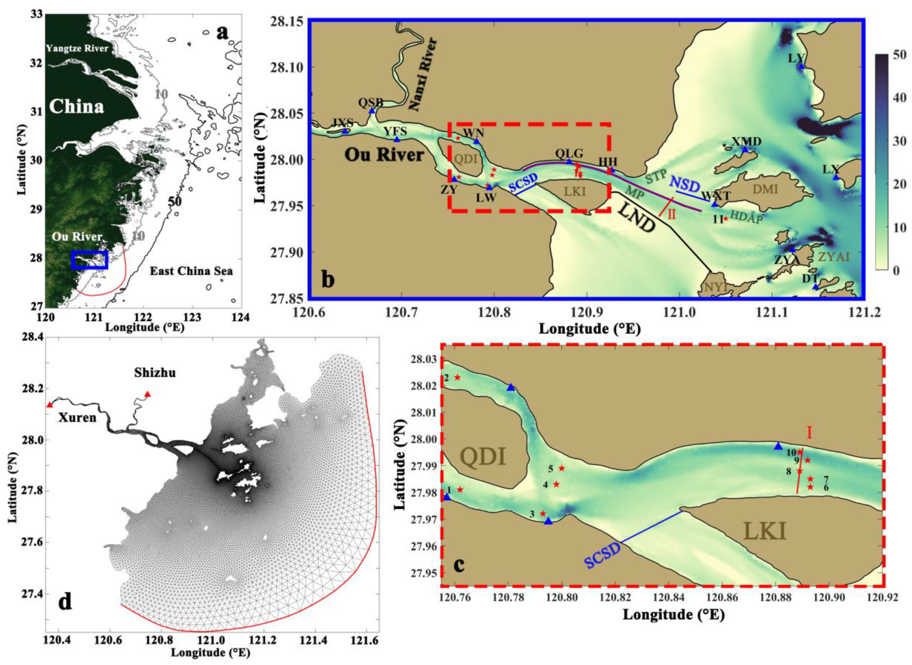
Figure 2.
(a) River discharge of the OR (blue) and the Yangtze River (red); shadow indicates the plum-rainy/typhoon season. (b) Measured elevation at the QLG tidal elevation station in Figure 1b (black line) and daily average OR discharge (blue bars) indicated by the blue box in (a); the period in red indicates the in situ measurement during spring tide and neap tide.

Figure 3.
Measured structures of (a,c,e,g) longitudinal, (b,d,f,h) lateral flows (filled contour, unit: m·s−1) and (i) salinity (filled contour, unit: psu) in the ORE during spring tide (landward looking). The flows are contoured in 0.1-m·s−1 intervals, and the salinity is in 1-psu intervals. Red dots indicate the measurement position. (a,b,i) are snapshots at high water slack, (c,d) are at maximum ebb tide, (e,f) are at low water slack, and (g,h) are at maximum flood tide. (j) Locations of shoal and DNC in Transect I (landward looking).
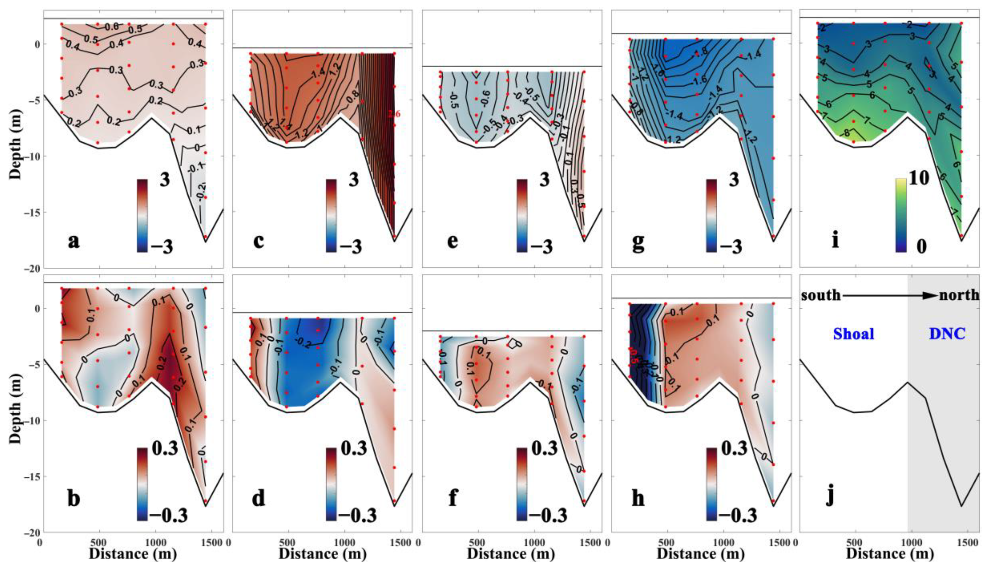
Figure 4.
Observed (dotted red line) and simulated (solid blue line) tidal elevations at the (a) HH, (b) WXT, and (c) ZYA tidal stations. The vertical averaged (d,e) current velocity and (f,g) current direction during (d,f) spring tide and (e,g) neap tide at No. 8 station.
Figure 4.
Observed (dotted red line) and simulated (solid blue line) tidal elevations at the (a) HH, (b) WXT, and (c) ZYA tidal stations. The vertical averaged (d,e) current velocity and (f,g) current direction during (d,f) spring tide and (e,g) neap tide at No. 8 station.
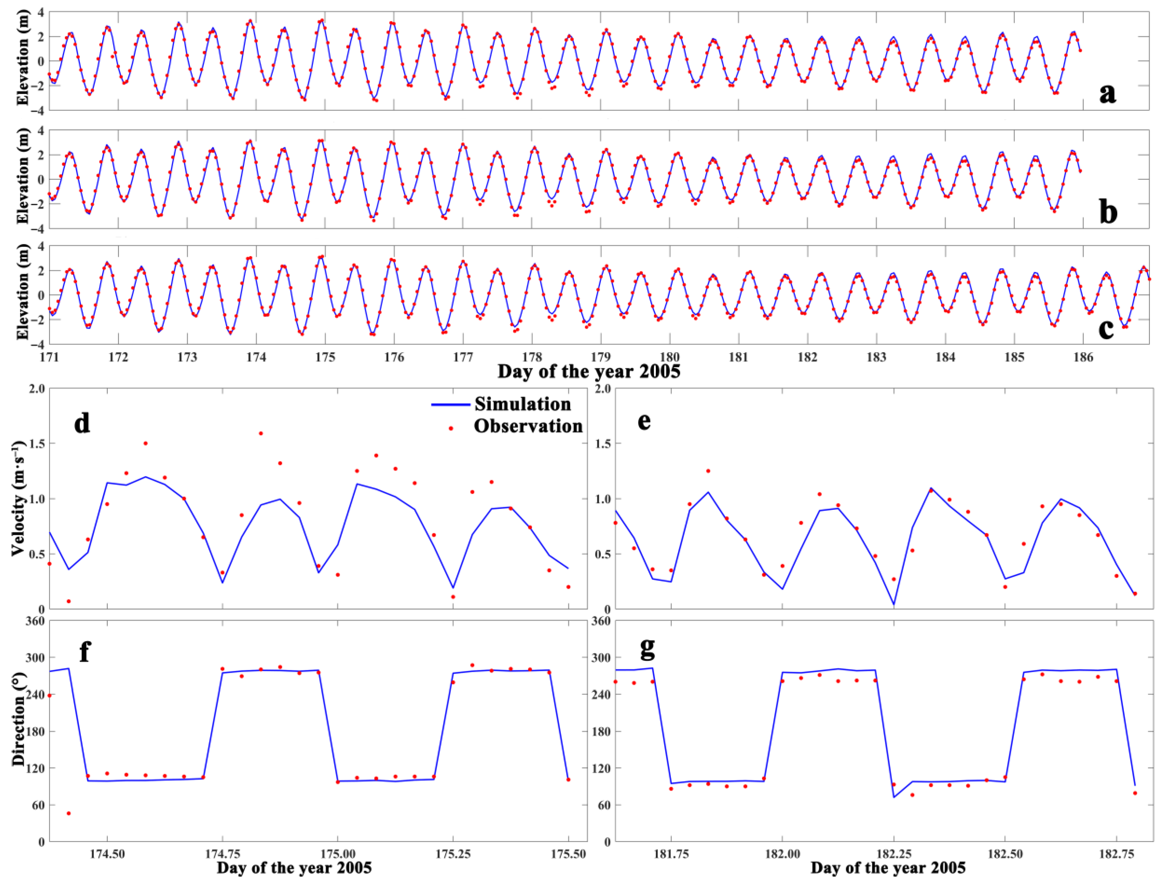
Figure 5.
Observed (dotted red line) and simulated (solid blue line) salinity at the (a) surface and (b) bottom at No. 8 station.
Figure 5.
Observed (dotted red line) and simulated (solid blue line) salinity at the (a) surface and (b) bottom at No. 8 station.
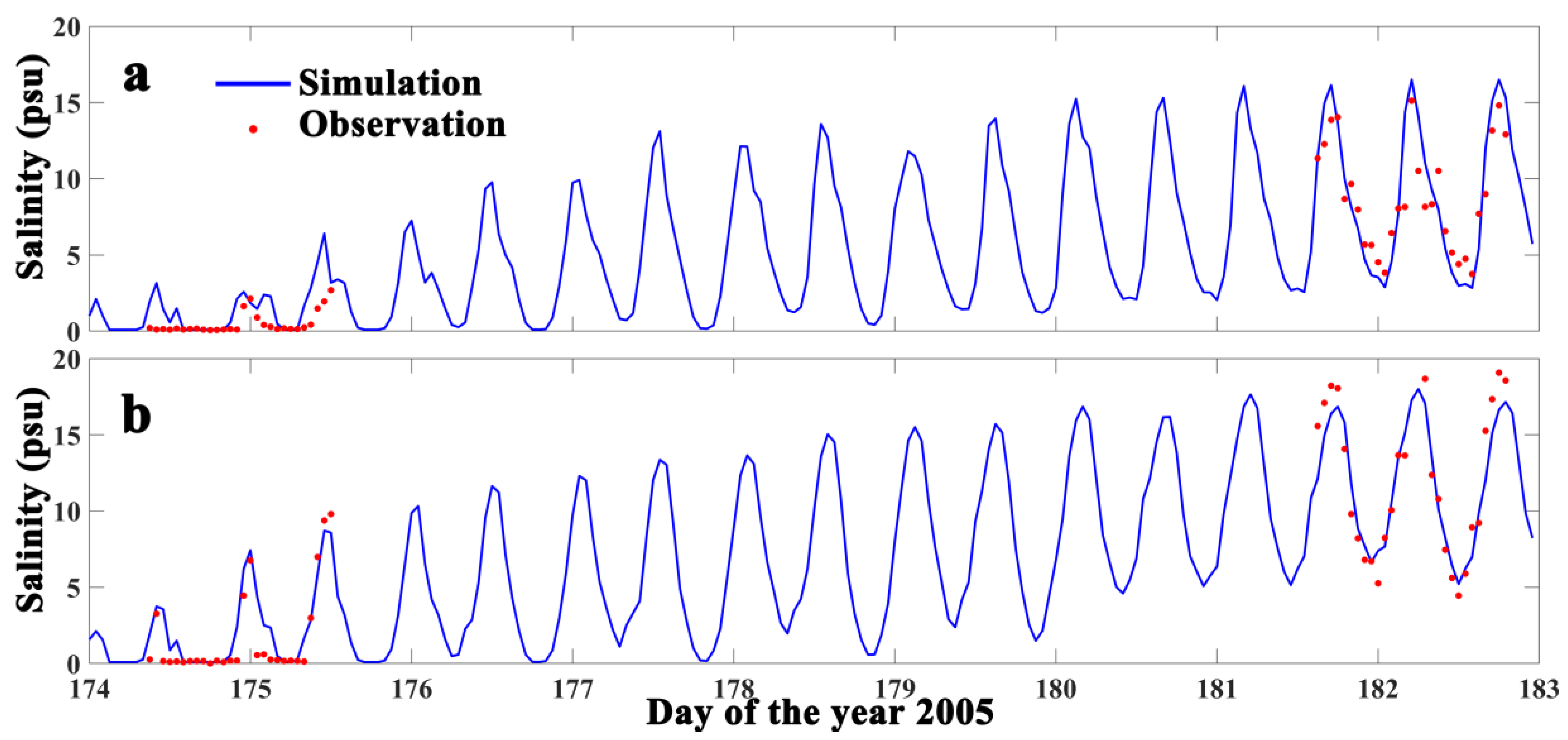
Figure 6.
(a) Two types of river discharge (blue lines) in the experimental runs. The black line is the modeled velocity (positive seaward) at the deepest DNC under the low-discharge condition (Run 2). Red indicates the ebb–flood tidal cycles used in this study. (b) Ebb–tidal-averaged and (c) flood–tidal-averaged salinities (filled contour with 1-psu intervals, unit: psu) of the along-channel section in Run 2. (d) The ebb–tidal-averaged and (e) flood–tidal-averaged salinities (filled contour with 1-psu intervals, unit: psu) of the along-channel section in Run 1. Red dashed lines indicate Transects I and II, respectively.
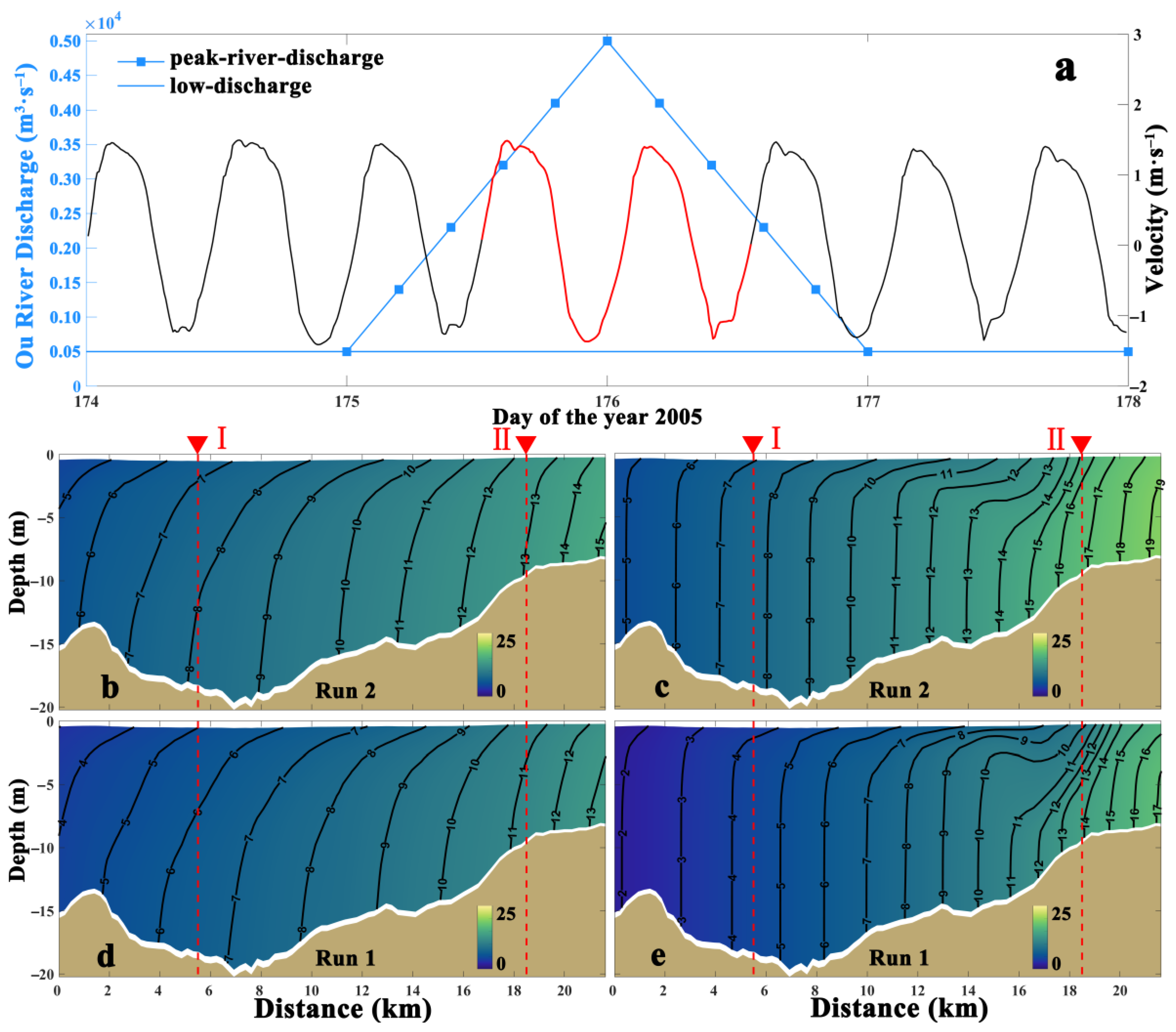
Figure 7.
Modeled transects (a–h) I and (i–p) II structures of salinity (filled contour, unit: psu) in Runs 1 and 2. The salinity is in 1-psu intervals. From the top panel to the bottom panel are snapshots at high water slack, maximum ebb tide, low water slack, and maximum flood tide (landward looking).
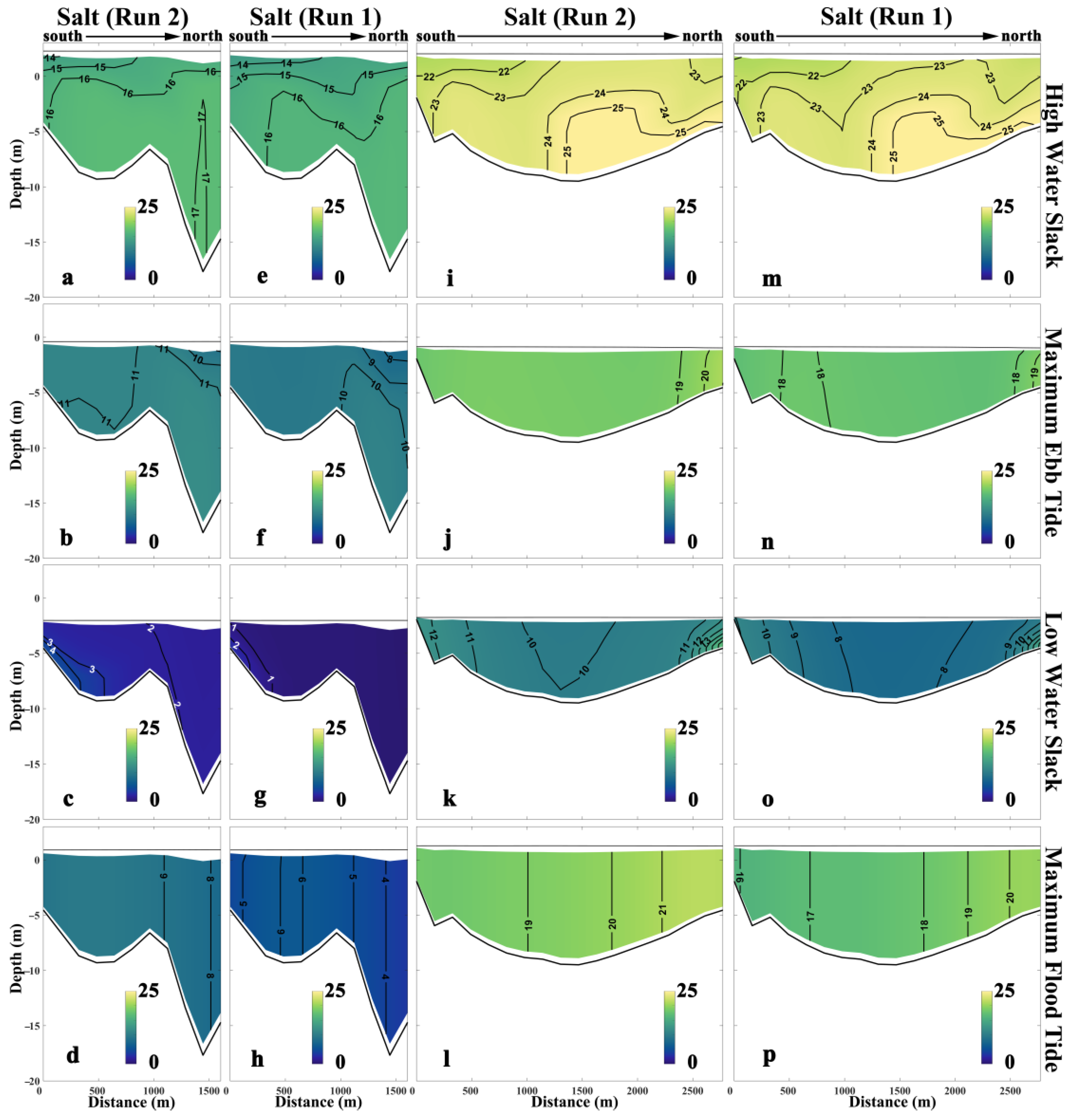
Figure 8.
Modeled transects (a–h) I and (i–p) II structures of (a–d,i–l) lateral flow in Run 2 and (e–h,m–p) lateral flow difference between Runs 1 and 2 (Run 1 minus Run 2) (filled contour, unit: m·s−1, positive indicates northward). The lateral flow is in 0.1 m·s−1 intervals and the lateral flow difference is in 0.05 m·s−1 intervals. From the top panel to the bottom panel are snapshots at high water slack, maximum ebb tide, low water slack, and maximum flood tide (landward looking).
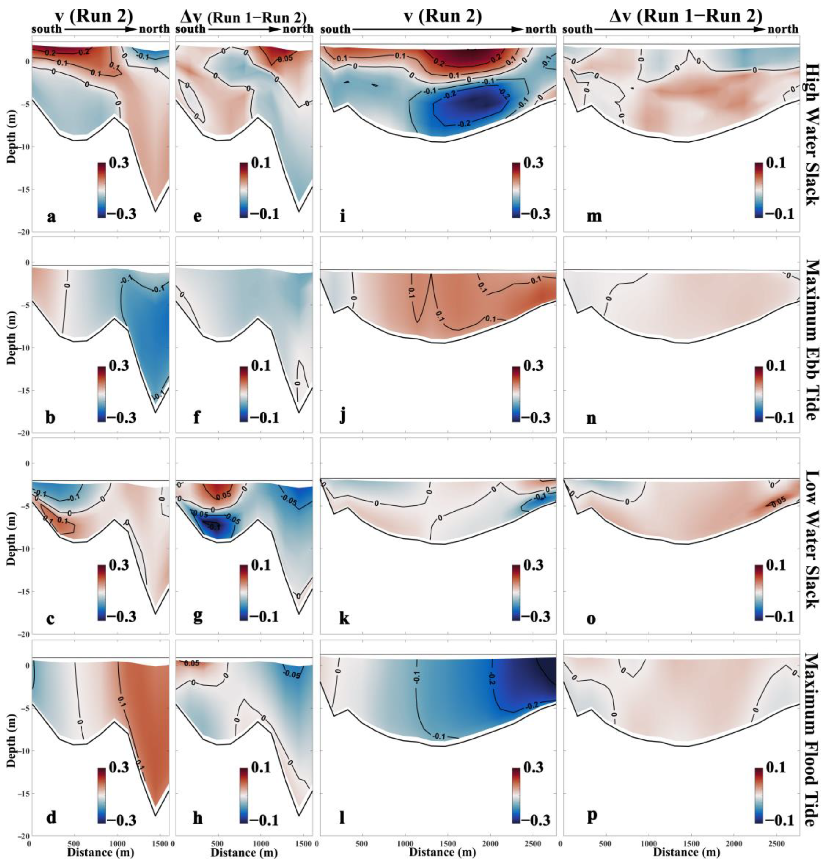
Figure 9.
Transect-averaged lateral velocity differences (color, unit: m·s−1) between each PRD run and Run 2 (each run minus Run 2) in Transects I (a) and II (b). The black contour line indicates 0.01 m·s−1. The solid red line is the division of the PRD influence period, and the red dotted line is the peak discharge moment.
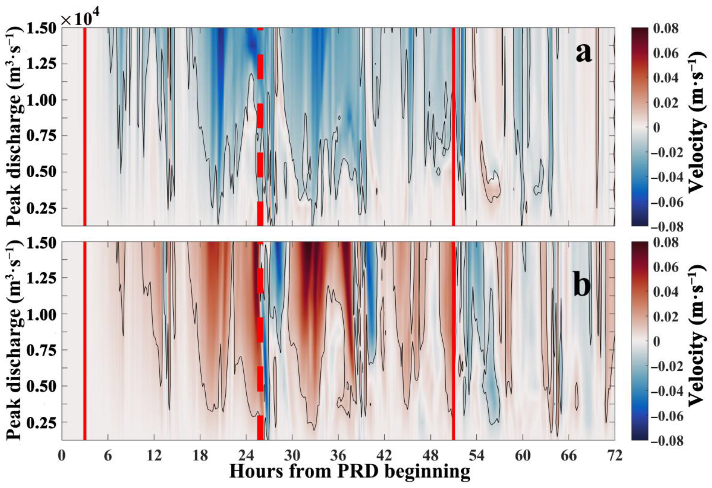
Figure 10.
Recovery times of (a,b) transect-averaged subtidal salinity, (c,d) transect-averaged subtidal longitudinal flow and (e,f) transect-averaged subtidal lateral flow in Transects I and II from left panels to right panels.
Figure 10.
Recovery times of (a,b) transect-averaged subtidal salinity, (c,d) transect-averaged subtidal longitudinal flow and (e,f) transect-averaged subtidal lateral flow in Transects I and II from left panels to right panels.
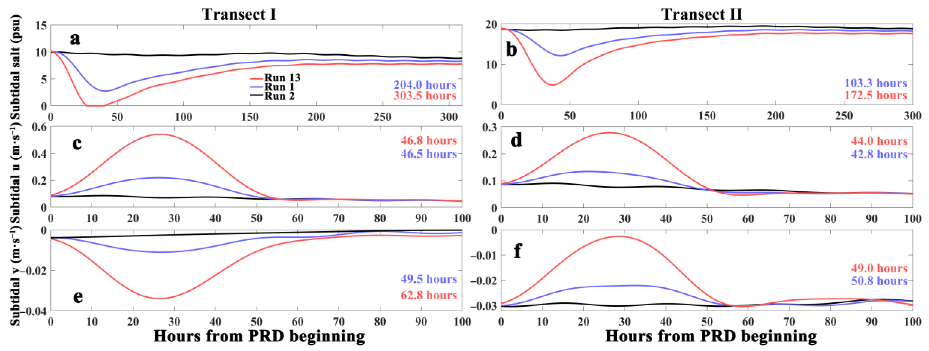
Figure 11.
Scatterplots of (a) salinity recovery time Tsalt approximated with Equation (4) versus , and (b) lateral recovery time Tv approximated with Equation (8) versus .
Figure 11.
Scatterplots of (a) salinity recovery time Tsalt approximated with Equation (4) versus , and (b) lateral recovery time Tv approximated with Equation (8) versus .


Table 1.
Skill score (SS) and correlation coefficient (CC) between the observed and simulated tidal elevation at different stations and their observation duration in 2005 (UTC +0800).
Table 1.
Skill score (SS) and correlation coefficient (CC) between the observed and simulated tidal elevation at different stations and their observation duration in 2005 (UTC +0800).
| Station | Observation Date | Day of the Year | SS | CC |
|---|---|---|---|---|
| JXS | 15 June–16 July | 166–197 | 0.952 | 0.978 |
| QSB | 20 June–5 July | 171–186 | 0.949 | 0.976 |
| YFS | 20 June–5 July | 171–186 | 0.954 | 0.975 |
| WN | 20 June–5 July | 171–186 | 0.971 | 0.983 |
| ZY | 20 June–5 July | 171–186 | 0.970 | 0.982 |
| LW | 20 June–5 July | 166–197 | 0.966 | 0.982 |
| QLG | 20 June–5 July | 171–186 | 0.979 | 0.987 |
| HH | 20 June–5 July | 171–186 | 0.980 | 0.987 |
| WXT | 20 June–5 July | 171–186 | 0.984 | 0.989 |
| LY | 20 June–6 July | 171–187 | 0.969 | 0.982 |
| XMD | 20 June–6 July | 171–187 | 0.982 | 0.988 |
| LX | 20 June–6 July | 171–187 | 0.945 | 0.969 |
| ZYA | 20 June–6 July | 171–187 | 0.986 | 0.990 |
| DT | 15 June–16 July | 166–197 | 0.978 | 0.988 |
Table 2.
Skill score (SS) and correlation coefficient (CC) between the observed and simulated west–east (U) and south–north (V) tidal currents at different stations.
Table 2.
Skill score (SS) and correlation coefficient (CC) between the observed and simulated west–east (U) and south–north (V) tidal currents at different stations.
| No. | Spring Tide | Neap Tide | ||||||
|---|---|---|---|---|---|---|---|---|
| U_SS | U_CC | V_SS | V_CC | U_SS | U_CC | V_SS | V_CC | |
| 1 | 0.901 | 0.924 | 0.815 | 0.895 | 0.778 | 0.915 | 0.802 | 0.934 |
| 2 | 0.862 | 0.926 | 0.693 | 0.857 | 0.894 | 0.931 | 0.707 | 0.912 |
| 3 | - | - | - | - | 0.932 | 0.942 | 0.608 | 0.756 |
| 4 | - | - | - | - | 0.967 | 0.953 | 0.763 | 0.927 |
| 5 | - | - | - | - | 0.920 | 0.954 | 0.802 | 0.951 |
| 6 | 0.942 | 0.939 | <0.20 | <0.20 | - | - | - | - |
| 7 | 0.908 | 0.932 | 0.821 | 0.912 | - | - | - | - |
| 8 | 0.939 | 0.938 | 0.658 | 0.870 | 0.972 | 0.952 | <0.20 | <0.20 |
| 9 | 0.737 | 0.915 | <0.20 | 0.466 | - | - | - | - |
| 10 | 0.860 | 0.924 | 0.789 | 0.921 | - | - | - | - |
| 11 | 0.822 | 0.880 | 0.276 | 0.561 | 0.886 | 0.917 | <0.20 | 0.577 |
“-” indicates no measurement at this tidal cycle.
Table 3.
Skill score (SS) and correlation coefficient (CC) between the observed and simulated salinity at different stations.
Table 3.
Skill score (SS) and correlation coefficient (CC) between the observed and simulated salinity at different stations.
| No. | Spring Tide | Neap Tide | ||||||
|---|---|---|---|---|---|---|---|---|
| Surface | Bottom | Surface | Bottom | |||||
| SS | CC | SS | CC | SS | CC | SS | CC | |
| 1 | * | * | * | * | 0.546 | 0.906 | 0.545 | 0.884 |
| 2 | * | * | * | * | 0.576 | 0.841 | 0.678 | 0.926 |
| 3 | - | - | - | - | 0.673 | 0.892 | 0.792 | 0.925 |
| 4 | - | - | - | - | 0.808 | 0.905 | 0.891 | 0.911 |
| 5 | - | - | - | - | 0.639 | 0.850 | 0.833 | 0.927 |
| 6 | <0.20 | 0.718 | 0.824 | 0.883 | - | - | - | - |
| 7 | <0.20 | 0.784 | 0.773 | 0.856 | - | - | - | - |
| 8 | <0.20 | 0.636 | 0.780 | 0.876 | 0.623 | 0.892 | 0.879 | 0.923 |
| 9 | <0.20 | 0.859 | 0.611 | 0.802 | - | - | - | - |
| 10 | <0.20 | 0.733 | 0.735 | 0.823 | - | - | - | - |
| 11 | <0.20 | 0.733 | 0.856 | 0.910 | 0.580 | 0.822 | 0.452 | 0.769 |
“-” indicates no measurement at this tidal cycle. “*” indicates the observed salinity approximately 0 psu.
Table 4.
Experiment configuration.
| Run | Discharge Type | Peak Discharge (m3·s−1) |
|---|---|---|
| 0 | Real condition | - |
| 1 | Peak river discharge | 5000 |
| 2 | Low-discharge | 500 |
| 3 | Peak river discharge | 1250 |
| 4 | Peak river discharge | 2500 |
| 5 | Peak river discharge | 3750 |
| 6 | Peak river discharge | 6250 |
| 7 | Peak river discharge | 7500 |
| 8 | Peak river discharge | 8750 |
| 9 | Peak river discharge | 10,000 |
| 10 | Peak river discharge | 11,250 |
| 11 | Peak river discharge | 12,500 |
| 12 | Peak river discharge | 13,750 |
| 13 | Peak river discharge | 15,000 |
Table 5.
Transect-averaged lateral momentum terms and change in RMS (unit: ×10−6 m·s−2) after tidal averages in Runs 1 and 2. Positive indicates northward.
Table 5.
Transect-averaged lateral momentum terms and change in RMS (unit: ×10−6 m·s−2) after tidal averages in Runs 1 and 2. Positive indicates northward.
| Transect I | Transect II | |||||
|---|---|---|---|---|---|---|
| Run 2 | Run 1 | Change RMS | Run 2 | Run 1 | Change RMS | |
| vt | 1.39 | 0.84 | 1.84 | −0.69 | −0.66 | 7.99 |
| −uvx−fu | 29.97 | 25.28 | 14.06 | −76.87 | −79.58 | 12.33 |
| Pty | −44.68 | −39.94 | 12.27 | 95.93 | 100.25 | 17.16 |
| Pcy | 28.74 | 26.65 | 7.35 | −30.31 | −29.46 | 12.84 |
| −vvx−wvz | −14.37 | −17.65 | 9.60 | 2.76 | 2.78 | 11.88 |
| (Kvvz)z | 1.55 | 5.37 | 6.59 | 8.03 | 6.04 | 10.21 |
| (Amvx)x+(Amvy)y | 0.18 | 1.13 | 2.29 | −0.23 | −0.69 | 2.77 |
Table 6.
Recovery time (unit: hour) of transect-averaged salinity (S), longitudinal (u) and lateral flow (v) after a PRD with peak discharge (unit: m3·s−1) shown in parentheses.
Table 6.
Recovery time (unit: hour) of transect-averaged salinity (S), longitudinal (u) and lateral flow (v) after a PRD with peak discharge (unit: m3·s−1) shown in parentheses.
| Run 3 (1250) | Run 4 (2500) | Run 5 (3750) | Run 1 (5000) | |||||||||
| S | u | v | S | u | v | S | u | v | S | u | v | |
| Transect I | 78.7 | 46.7 | 38.0 | 140.8 | 46.5 | 47.7 | 175.8 | 46.7 | 49.2 | 204.0 | 46.5 | 49.5 |
| Transect II | 32.3 | 44.3 | 44.2 | 62.0 | 43.3 | 50.7 | 89.3 | 43.3 | 51.8 | 103.3 | 42.8 | 50.8 |
| Run 6 (6250) | Run 7 (7500) | Run 8 (8750) | Run 9 (10,000) | |||||||||
| S | u | v | S | u | v | S | u | v | S | u | v | |
| Transect I | 231.3 | 46.5 | 55.2 | 253.7 | 46.7 | 70.8 | 275.7 | 46.8 | 71.0 | 293.0 | 46.8 | 75.3 |
| Transect II | 116.8 | 42.7 | 60.5 | 126.5 | 42.5 | 51.8 | 135.0 | 42.5 | 52.7 | 143.2 | 42.7 | 48.0 |
| Run 10 (11,250) | Run 11 (12,500) | Run 12 (13,750) | Run 13 (15,000) | |||||||||
| S | u | v | S | u | v | S | u | v | S | u | v | |
| Transect I | 302.2 | 46.8 | 67.7 | 302.5 | 46.8 | 64.2 | 303.0 | 46.8 | 62.0 | 303.5 | 46.8 | 62.8 |
| Transect II | 151.3 | 42.8 | 49.3 | 158.8 | 43.3 | 48.0 | 166.2 | 43.7 | 49.2 | 172.5 | 44.0 | 49.0 |
Publisher’s Note: MDPI stays neutral with regard to jurisdictional claims in published maps and institutional affiliations. |
© 2020 by the authors. Licensee MDPI, Basel, Switzerland. This article is an open access article distributed under the terms and conditions of the Creative Commons Attribution (CC BY) license (http://creativecommons.org/licenses/by/4.0/).
Share and Cite
MDPI and ACS Style
Yan, Y.; Song, D.; Bao, X.; Ding, Y. The Response of Lateral Flow to Peak River Discharge in a Macrotidal Estuary. Water 2020, 12, 3571. https://doi.org/10.3390/w12123571
AMA Style
Yan Y, Song D, Bao X, Ding Y. The Response of Lateral Flow to Peak River Discharge in a Macrotidal Estuary. Water. 2020; 12(12):3571. https://doi.org/10.3390/w12123571
Chicago/Turabian StyleYan, Yuhan, Dehai Song, Xianwen Bao, and Yang Ding. 2020. "The Response of Lateral Flow to Peak River Discharge in a Macrotidal Estuary" Water 12, no. 12: 3571. https://doi.org/10.3390/w12123571
Note that from the first issue of 2016, this journal uses article numbers instead of page numbers. See further details here.