Reconstruction of River Topography for 3D Hydrodynamic Modelling Using Surveyed Cross-Sections: An Improved Algorithm

Abstract

Multidimensional hydrodynamic modelling becomes tricky when lacking the bathymetric data representing the continuous underwater riverbed surface. Light detection and ranging (LiDAR)-based and radar-based digital elevation models (DEMs) are often used to build the high-accuracy floodplain topography, while in most cases the submerged riverbed could not be detected because both radar and LiDAR operate at wavelengths that cannot penetrate the water. Data from other sources is therefore required to establish the riverbed topography. The inundated river channel is often surveyed with an echo sounder to obtain discrete cross-section data. In this context, an improved algorithm based on the classic flow-oriented coordinates transformation is proposed to generate the riverbed topography using surveyed cross-sections. The dimensionless channel width (DCW) processing method is developed within the algorithm to largely increase the prediction accuracy, especially for the meandering reaches. The generated riverbed topography can be merged with the floodplain DEM to create an integrated DEM for 2D and 3D hydrodynamic simulations. Two case studies are carried out: a benchmark test in the Baxter River, United States, with carefully surveyed channel–floodplain topographic data to validate the algorithm, and a 3D hydrodynamic modelling-based application in Three Gorges Reservoir (TGR) area, China. Results from the benchmark case demonstrate very good consistency between the created topography and the surveyed data with root mean square error (RMSE) = 0.17 m and the interpolation accuracy was increased by 55% compared to the traditional method without DCW processing. 3D hydrodynamic modelling results match the observed field data well, indicating that the generated DEM of the TGR area was good enough not only to predict water depths along the tributary, but also to allow the hydrodynamic model to capture the typical features of the complex density currents caused by both the topography of the tributary estuary and the operation rules of TGR.

1. Introduction

Recent decades have witnessed a significant upgrade of computing power as well as numerical schemes, which largely facilitated the practical application of two- and three-dimensional (2D and 3D) hydrodynamic models. Today multidimensional models, considered as essential and efficient tools in river system study and exploitation, are widely used in flood risk assessment [1], river sediment dynamics [2], aquatic ecosystem [3] and reservoir management [4].

To set up a 2D or 3D model, the first step, in general, is generating a computational mesh containing real-world topographic information of both the underwater riverbed and the dry land. The z-value, i.e., the elevation of every mesh node, is normally assigned through the direct interpolation of topographic data surveyed in situ or collected by other means. To what extent the mesh reflects reality is mostly determined by the resolution and magnitude of the topographic data, when the mesh structure remains fixed. Numerous studies have indicated that the irregularity and anisotropic characteristic of riverbeds and floodplains could strongly influence the response of 2D and 3D hydrodynamic models [5,6,7]. In consequence, a sufficiently fine digital elevation model (DEM) is vital for 2D and 3D hydrodynamic model construction and application.

Airborne interferometric radar and its data products, such as Shuttle Radar Topography Mission (SRTM) 1 arc-second global DEM [8], have been widely used to represent large scale dry areas, while light detection and ranging (LiDAR) nowadays is often used to generate topographic maps with higher resolution [9]. For example, aerial laser scanning (ALS) and terrestrial laser scanning (TLS) were used to generate DEMs for geomorphology studies of river systems [10,11]. Unfortunately, both aforementioned techniques are unable to measure the submerged riverbed (channel zone) topography because radar signals cannot penetrate the water surface and the latter still has limitations in bathymetry applications [12,13,14]. An alternative and classic way to survey the submerged bathymetry is by echo sounding (or sonar), which is quite useful to obtain riverbed terrain with fine resolution. However, using an echo sounder with a global navigation satellite system (GNSS) receiver to obtain the point-cloud bathymetric data of the whole submerged area would still be time-consuming and expensive when it comes to large-scale river systems, especially for mountainous rivers in high latitudes or remote areas. Other than the high-resolution point-cloud representation of the riverbed terrain, surveyed cross-section data are much easier to access and have been widely used. Furthermore, the cross-section data may be obtained directly from watershed management institutes through scientific collaboration projects, or even for free as a certain type of public resource.

Since the surveyed cross-section data is often available for river systems, developing an algorithm to generate the continuous 3D riverbed topography using cross-section data becomes crucial, the result of which can then be merged with LiDAR- or radar-based floodplain and dry region DEMs to create a new DEM that covers the whole computational domain of the model. The most important and inevitable issue that needs to be resolved is to cope with the irregularity, i.e., the meandering and sinuous characteristic of the river channel, due to the fact that commonly used surface interpolation methods are unable to yield a satisfying riverbed surface using sparsely scattered cross-sections under the real-world Cartesian coordinate system [15]. Several studies have investigated this issue from different kinds of perspectives, while almost all of them adopted the same transformation method between a Cartesian (x, y) coordinate system and a curvilinear orthogonal (s, n) coordinate system, to facilitate the interpolation process. Merwade et al. [16] offered a transformation methodology based on the commercial software ArcGIS environment [16]; later they proposed a modified inverse distance weighting method accounting for the river anisotropy, which outperformed the commonly used spatial interpolation methods [17]. Dysarz [18] adopted the same coordinates transformation and developed an ArcGIS toolbox for river bathymetry reconstruction. Instead of developing an algorithm tightly bound to a specific software environment, Legleiter and Kyriakidis [19] introduced more flexible and compatible transformation procedures between Cartesian and channel-fitted coordinates from the mathematical perspective.

Although interest in the exploration of riverbed reconstruction methods is growing, little attention has been paid to how to improve the results when only a limited number of surveyed cross-sections are available, e.g., intervals larger than two to three times the channel width. In addition, the influence of the generated DEM on flood inundation mapping in 2D hydrodynamic modelling has been carefully investigated [20,21,22], however, its impacts on 3D hydrodynamic modelling performance are rarely looked into.

Motivated by the necessity to carry out 2D or 3D modelling of river systems and reservoirs where only sparsely surveyed cross-sectional data are available, on the basis of the mathematical methodology described by Legleiter and Kyriakidis [19], in this paper we propose a robust algorithm for river topography reconstruction in which the innovative dimensionless channel width (DCW) processing was implemented to largely improve the interpolation accuracy and smooth the merging process with the floodplain DEM as well; thus the uncertainty introduced by manual handling of void or overlapping areas was avoided. This paper is organized as follows. Section 2 explains the proposed algorithm in detail for riverbed topography reconstruction using cross-sections. Section 3 carries out a benchmark test in a well-surveyed river and floodplain area to validate the algorithm. Section 4 presents the application of the algorithm in a typical tributary and the main stream of the Three Gorges Reservoir with 3D hydrodynamic modelling results compared against field data; finally brief conclusions are drawn in Section 5.

2. Methodology

2.1. Algorithm Definitions

The algorithm presented herein adopted the classic coordinates transformation between Cartesian and curvilinear orthogonal coordinate systems as shown in Figure 1a; the transformation had already been demonstrated by previous researchers [16,19,23]. Basically, the S-N coordinate system is comprised of a curvilinear S axis representing the river flow direction and the N axis normal to the S axis. In this paper the thalweg was chosen as the S axis because it marks the natural direction of a watercourse. As depicted in Figure 1a, two arbitrary points ${\mathrm{P}}_1$ and ${\mathrm{P}}_2$ located within the channel whose Cartesian coordinates are ($x_1$, $y_1$) and ($x_2$, $y_2$), could be defined by ($s_1$, $n_1$) and ($s_2$, $-n_2$) respectively after calculating their S-N coordinates. The first coordinate s is the curvilinear length along the S axis and the second coordinate n means the shortest distance from the related point to the S axis. More importantly, the channel widths along the S axis are calculated to obtain the dimensionless width representation of the entire river channel, as demonstrated in Figure 1b,c. Because of the dimensionless channel width (DCW) processing, the anisotropic and irregular natural river was reshaped into a virtual rectangular channel ready for further processing.

2.2. Procedure for River DEM Reconstruction

The whole procedure for river topography reconstruction is composed of four main steps. First, transform Cartesian coordinates of cross-sections into the S-N coordinate system. Then, using the calculated channel widths along the S axis to obtain the rectangular river channel which is dimensionless along the N axis. Third, fill the gap between adjacent cross-sections by linear interpolation and transform the interpolated rectangular riverbed back to the real-world Cartesian coordinate system. Finally, the generated riverbed topography and floodplain DEM were merged into an integrated new DEM. We elaborated on the methodology to solve the problem step-by-step as listed below, and summarized the overall reconstruction process into the flow chart shown in Figure 2.

Step 1

Data preparation. Preliminary treatment is carried out to obtain the desirable input data, i.e., the surveyed cross-sectional data and floodplain DEM data from the LiDAR survey or other freely accessible source. Use coordinate conversion to make sure the two datasets have the same georeferencing, if needed.

Step 2

Thalweg and river banks identification. Pick out the lowest points of every cross-section as the initial discrete thalweg. Left and right river banks are either extracted from the floodplain DEM or manually depicted using a map provider such as Google Maps.

Step 3

Thalweg digitization. Filter the coordinates of the initial thalweg points to smooth the data and reduce the noise introduced by manual selection, then use cubic splines to fit the filtered thalweg points. After that, resample the S axis with a large number of vertices equidistant from each other, to parameterize the S axis.

Step 4

Bank line resampling. Use cubic splines to parameterize the sequence of points representing the river bank, then resample the bank line into equally spaced vertices finer than the resampled S axis, to ensure the successful calculation of channel widths.

Step 5

Calculation of the (s, n) coordinates and DCW processing. As shown in Figure 1b, calculate normal vectors at adjacent vertices $S_i$ and $S_{i+1}$ to compose the blue dotted searching window of the S axis segment [$S_i$, $S_{i+1}$]. Inside the window calculate the mean distance of all bank line points to the S axis as the right half channel width $w_2$ corresponding to this segment [$S_i$, $S_{i+1}$]. Then compute the (s, n) coordinates of each cross-section point captured inside the window and implement DCW processing. Take point ${\mathrm{P}}_2$ as an example, the s coordinate denoted as $s_2$ is the curvilinear length from the S–N origin ($s_0$, $n_0$) to the intersection of normal vector $\overrightarrow{n_2}$ and S axis; the dimensionless n coordinate of ${\mathrm{P}}_2$ could be denoted by $-n_2/w_2$.

Step 6

Linear interpolation. Linearly interpolate the (s, n, z) coordinates of all the cross-section points inside the regular river channel bounded by $-1\le n\le +1$ and $0\le s\le s_{max}$ to obtain the raster or regular mesh representing the riverbed topography with dimensionless channel widths.

Step 7

Backward transformation. Transform the coordinates of all the nodes back into (x, y, z) to acquire the riverbed topography under the real-world Cartesian system. A finite difference approach was used to acquire the functions below for calculating the Cartesian coordinates (x, y) of an arbitrary point inside the rectangular river channel with known (s, n) coordinates.

$$x=x_{t }\left(s\right)-n{w}_i\frac{d{y}_t\left(s\right)}{ds}$$

(1)

$$y=y_t\left(s\right)+n{w}_i\frac{d{x}_t\left(s\right)}{ds}$$

(2)

where, $x_{t }\left(s\right)$ and $y_t\left(s\right)$ denote the Cartesian coordinates of the intersection point of the normal vector $\overrightarrow{n}$ and the S axis, $w_i$ denotes the half channel width associated with the S axis segment [$S_i$, $S_{i+1}$], where the arbitrary point was located.

Step 8

Merging with floodplain DEM. Cut out the elements between left and right river banks in the floodplain DEM and then merge them with the generated riverbed point cloud; these two datasets would perfectly meld with each other since they share the same boundary owing to DCW processing. Now a new DEM including both submerged and floodplain topography is created, ready for a wide utilization in hydrological and hydrodynamic numerical modelling.

3. Benchmark Test

3.1. Benchmark Description

The algorithm was first tested for the Baxter River located in Modesto, California, United States, where both the river channel and floodplain area had been carefully surveyed and all the data needed for algorithm validation were freely accessible from Arturo Leon’s research group website [24], including the surveyed cross-sectional data, the contour map, triangular irregular networks (TIN) data and the aerial image. As presented in Figure 3a, the 1.4 km long river reach, 40 m wide on average, turning 90 degrees from westward to southward, was chosen for the benchmark test. The water depth was around only a few meters due to the flat terrain and the annual average discharge provided by United States Geological Survey (USGS) was 37.8 m³/s (USGS gauge 11,290,000). Fourteen surveyed cross-sections were to be used by the proposed algorithm to generate the submerged topography. Figure 3b shows the surveyed point cloud extracted from contour map and TIN nodes with a finest horizontal resolution less than 1 m. The proposed algorithm can be validated by comparing the generated topography with the surveyed point cloud data and statistically analyzing the predicted errors. Two other reconstructing methods, i.e., direct linear interpolation and coordinates transformation without DCW processing were considered to evaluate the performance of the proposed algorithm in a comprehensive way.

3.2. Reconstruction of Baxter River Channel Topography

Cross-sections of the selected Baxter River reach in Figure 3a were used to generate the river channel topography, which was then compared against the surveyed point cloud data in Figure 3b to evaluate the performance of the algorithm. The overall reconstruction process is illustrated in Figure 4.

3.2.1. Thalweg and River Banks Digitization

The digitized river banks were essential in this algorithm for providing channel width data during DCW processing. Normally river banks could be easily identified and extracted from the floodplain DEM or aerial image since the edge between water surface and dry land was always noticeable. In this benchmark test Baxter River banks were manually drawn along the edge of river channel using high-resolution floodplain DEM data. In Figure 4a the initially defined river banks and thalweg are represented by blue squares and red circles, respectively. To digitize these geographic features, a Savitzky–Golay filter [25] was applied to three data sets separately to smooth the initial digital representation. Three resampled cubic splines were then used to fit the filtered river banks and thalweg points as shown in Figure 4b; each cubic spline was equally resampled by a specific number of points. The detailed resampling information is listed below in

Table 1. Thalweg and river banks spline resampling information.

Name	Number of Points Used	Segment Length (Meter)
thalweg	5001	0.34
left bank	22,001	0.048
right bank	40,001	0.048

; river bank splines were resampled to a much finer degree than the thalweg spline to ensure that every thalweg segment was able to capture a few bank spline vertices for channel width calculation, as displayed in Figure 1b.

3.2.2. Coordinates Transformation and DCW Processing

The digitized and evenly resampled thalweg spline was then used as the curvilinear S axis whose positive direction was defined toward downstream. Starting from the origin (0, 0) of S-N coordinate system, i.e., the first thalweg point upstream, the searching window displayed in Figure 1b slid along the S axis to scan the left river channel twice. First the digitized left bank was scanned to calculate left channel width of every corresponding S axis segment; the second scan was aimed at calculating the (s, n) coordinates of all the cross-section points inside the left river channel. The data sets obtained from the scanning above were processed by the DCW algorithm to achieve the lateral dimensionless representation of cross-sections inside the left river channel under the S-N system. The whole processing was then repeated on the other side of the S axis to complete the coordinates transformation and the DCW processing of all the cross-section points. Figure 4c,d shows the transformed cross-sections before and after DCW processing, respectively.

3.2.3. Interpolation and Backward Transformation

The s, n, z coordinates of cross-sections in Figure 4d were linearly interpolated on a regular rectangular mesh under S-N coordinate system as shown in Figure 4e. Due to the anisotropy of the natural riverbed that topography changes more sharply in the cross-sectional direction than in the longitudinal direction, the mesh was generated with a 5 m × 0.005 resolution sufficiently fine along the N axis direction to account for the anisotropic feature of the river reach. Then a backward transformation was carried out to convert every node of the rectangular channel back into the real-world Cartesian system to create the Baxter River channel topography presented in Figure 4f.

3.3. Algorithm Performance Evaluation

In order to fully evaluate the performance of the proposed algorithm for riverbed topography reconstruction, two other commonly used scenarios, i.e., direct linear interpolation (DLI) and coordinate system transformation (CST) were designed to compare against the proposed algorithm which can be denoted as CST + DCW. DLI used linear interpolation of cross-sections directly under a Cartesian system to create the river channel topography, while CST used linear interpolation of cross-sections under a S-N system after coordinates transformation as shown in Figure 4c, without further DCW processing.

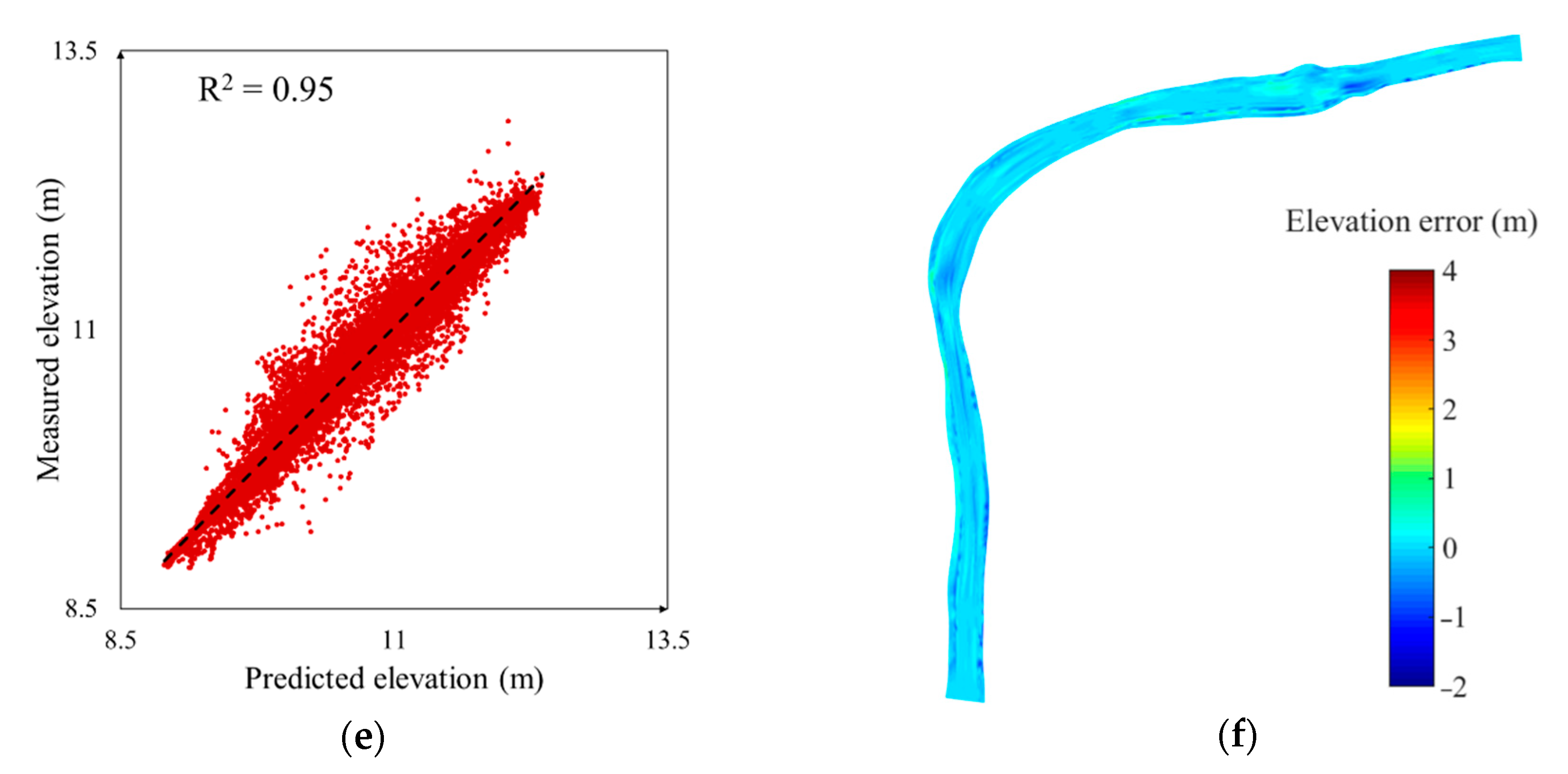
Since the riverbed topography created by different scenarios did not always share the same resolution or boundary with the surveyed point cloud data, validation of the predicted topography cannot be done directly. To make the comparison between the predicted and measured data easier, and more importantly, to avoid the false precision introduced by further interpolation of the measured point cloud, Delaunay triangulation was used for 5623 measured points between the digitized river banks, to generate the mesh in standard format for result demonstration. That means that the riverbed topography created by different scenarios would be interpolated into the standard mesh to form the one-to-one relationship between predicted and measured elevation data. In this context, the predicted versus measured values from different scenarios is regressed with the calculated coefficient of determination (R²) as illustrated in Figure 5a–c; the spatially distributed error in riverbed elevation resulted from different scenarios are depicted in Figure 5d–f.

$$MAE=\frac{1}{N}{\displaystyle \sum }_{i=1}^N\left|z_{i, predicted}-z_{i,measured}\right|$$

(3)

$$RMSE=\sqrt{\frac{1}{N}{\displaystyle \sum }_{i=1}^N{\left(z_{i,predicted}-z_{i,measured}\right)}^2}$$

(4)

The mean absolute error (MAE) and root mean square error (RMSE) of the predicted topography are employed as listed in Equations (3) and (4),$z_{i,predicted}$ and $z_{i, measured}$ are the predicted and measured elevation data at the ith node, respectively, and N is the number of nodes of the standard mesh. The results of MAE and RMSE are listed in

Table 2. Errors of the predicted riverbed elevation for the Baxter River reach.

Scenario	MAE (m)	RMSE (m)
DLI	0.636	1.09
CST	0.173	0.38
CST+DCW	0.106	0.17

.

From Figure 5 and Table 2 it is evident that DLI yields the worst result among the three reconstruction methods, it is noteworthy that although DLI fails to correctly predict the topography in the curved middle reach, it works quite well for the upper reach where the river channel is relatively straighter and there are more surveyed cross-sections, almost parallel to each other, than the middle and lower reach; this indicates that linear interpolation only works when dealing with straight regular river channels with parallel cross-sections. The idea of DCW processing proposed in this paper was also inspired by the result from DLI, that is to reduce all terrain-related irregularity and anisotropy to a minimum before carrying out linear interpolation with sparsely surveyed data.

Compared to DLI, both CST and CST+DCW show the ability to cope with the curved river channel, largely reducing the MAE and RMSE of constructed topography and raising R² at the same time. Nevertheless, CST overestimates the elevation of the area near the left bank in the middle reach for about 4 m, according to Figure 5d. The error caused by traditional CST method has been successfully eliminated by the proposed CST + DCW algorithm as shown in Figure 5f. In addition, the RMSE is reduced from 0.38 m to 0.17 m and R² is increased from 0.82 to 0.95 owing to the DCW processing. The algorithm proposed in this paper was proven to be capable of generating more accurate riverbed topography than traditional methods using surveyed cross-sections, during which the DCW processing plays a significant role in further increasing the interpolation accuracy.

4. Application in 3D Hydrodynamic Modelling

4.1. New DEM Generation

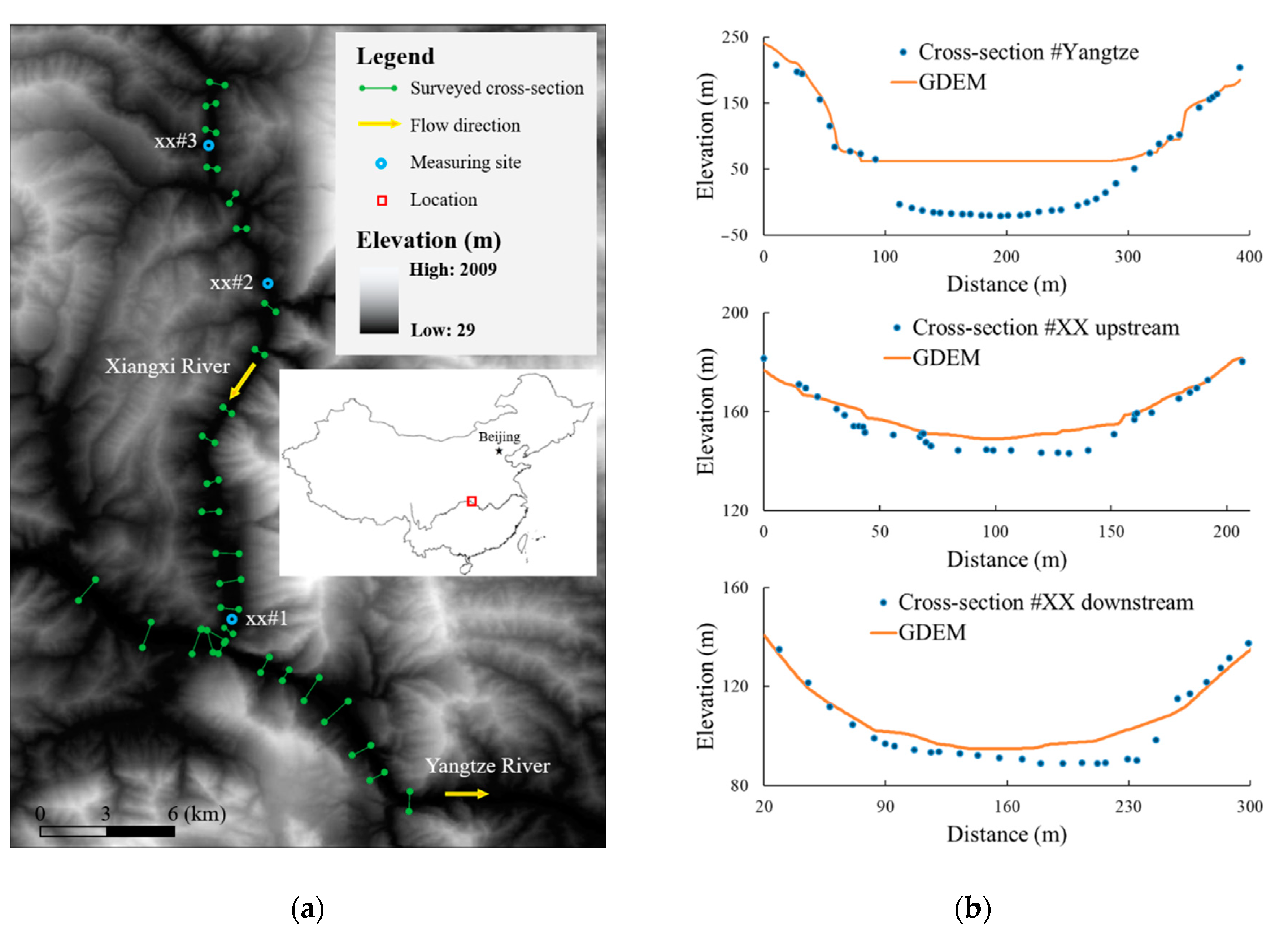
After the validation in the benchmark test, the proposed algorithm was then applied to the three-dimensional hydrodynamic modelling in the Three Gorges Reservoir (TGR) area in China, where the submerged topography required for computational mesh establishment was absent. Data available for topography reconstruction is demonstrated in Figure 6a; there are 29 field surveyed cross-sections distributed along the Yangtze River and its southward flowing tributary, the Xiangxi River, while the background DEM with 1 arc-second (about 30 m) resolution is freely accessible from the Advanced Spaceborne Thermal Emission and Reflection Radiometer Global DEM (ASTER GDEM) website [26]. To better understand the differences between the two data sets, three cross-sections were selected to compare the elevations as shown in Figure 6b. The upper figure demonstrates the comparison at one of the cross-sections on the Yangtze River and it is clear that the DEM derived by radar-based technology, as expected, results in a flat bottom characterizing the water surface in the middle of the river channel. The absent topographic information under the water surface can then be complemented by the surveyed cross-sections. The other two cross-sections from the upstream and downstream Xiangxi River display the similar phenomenon, with smaller elevation differences in the channel due to the much smaller flow discharge and water depth compared to the main stream. Despite the fact that the two data sets are coming from different sources, the surveyed cross-sections and GDEM have shown acceptable consistency of elevation in the dry area, indicating the smooth merging of reconstructed riverbed and DEM data.

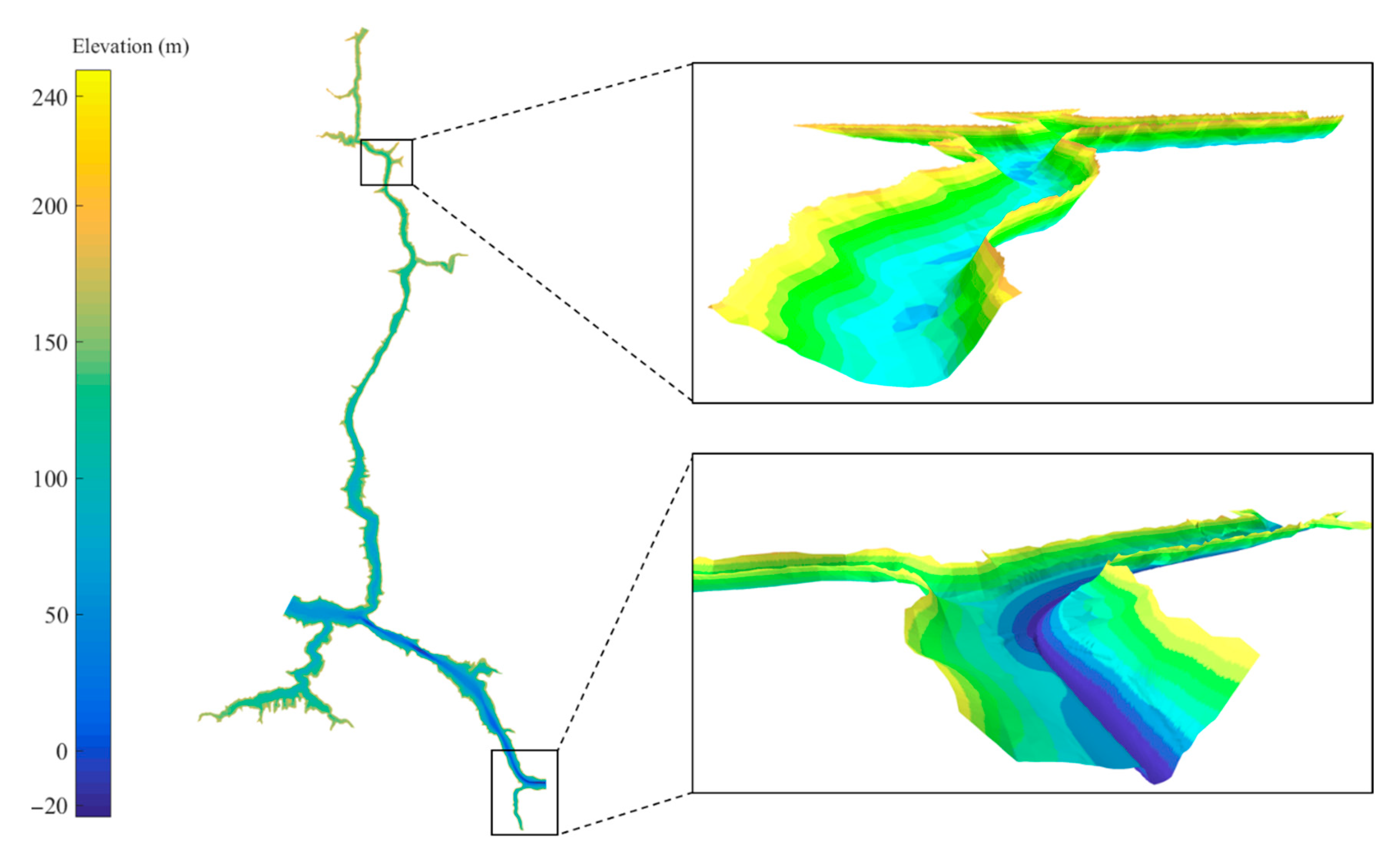
Since the TGR area consists of two river reaches, the riverbed topography of the Xiangxi River and Yangtze River were constructed separately by the proposed algorithm, then a new DEM covering the whole computational domain was created by merging the riverbed topography data with the DEM, as shown in Figure 7. Two insets of the new DEM display the upstream view of the Yangtze River and the downstream view of the meandering Xiangxi River; from the details it can be seen that the reconstructed river channels smoothly and accurately fit within the surrounding DEM.

4.2. Model Description

Based on the new DEM in the real-world Cartesian coordinate system, an unstructured triangular finite element mesh was generated to represent the computational domain. The open-source three-dimensional hydrodynamic model, TELEMAC-3D, was used to simulate the unique flow pattern observed along the Xiangxi River, a typical tributary subject to the impoundment and operation of Three Gorges Dam (TGD). It is located in the Hubei Province of China and flows across an area between 110.74° to 110.81° E and 30.96° to 31.25° N. As one of the Yangtze River tributaries, the Xiangxi River is about 36 km long with an annual average discharge around 57.4 m³/s. Since its confluence with the Yangtze River is only about 30 km away from the TGD upstream, the water level of Xiangxi River is almost synchronous with the operational water level before the TGD, varying between 145 to 175 m.

During the impounding period the water level before the TGD keeps rising, leading to the main stream flowing back into the tributary, moreover, as shown in Figure 7, the angle between the main stream and the tributary at the confluence also simplifies this backward current movement from a topographic perspective. Liu [27,28,29,30] and his research group attributed the occurrence of density currents to the water temperature difference between the Yangtze River and its tributary, as the water temperature of the Xiangxi River rising into the northern mountains is often lower than that of the Yangtze River. The character of this unique flow regime and its impact on river dynamics, water quality and aquatic ecosystem of the Xiangxi River has drawn significant interest from numerous researchers [31,32,33].

Details on the model, an introduction and governing equations for TELEMAC-3D can be found in Hervouet [34] or the theory guide for the model [35]. Boundary conditions of the simulation period from 6 January 2010 through 18 January 2010 are presented in Figure 8. Both inlets of the upstream Yangtze River and the Xiangxi River were set as the upper boundaries with inflow hydrographs and water temperature variations provided in Figure 8a,b, respectively. Air temperature variations of the area are shown in Figure 8b as well. The model takes the heat exchange between the air and water interface into account because water temperature is one of the key factors that determines the flow pattern of the density currents [27,29]. The outlet of the computational domain was set as the lower boundary, with the water elevation hydrograph shown in Figure 8c. All the data were obtained either from the local hydrological and meteorological station or from the historical data of the TGD operation on the China Three Gorges Corporation’s website [36]. The simulated 3D velocity field on 16 January 2010 was extracted from the model output to compare with field data, which was collected by an acoustic doppler velocimeter (ADV) from the water surface to the bottom at sufficiently fine intervals. On 16 January 2010 measurements were carried out at three different spots denoted as xx#1, xx#2 and xx#3 along the Xiangxi River to obtain vertical velocity profiles for the lower reach, middle reach and upper reach, respectively; the measuring sites are shown in Figure 6a. The model went through a warm-up time of 30 days (time in the model) to establish the initial hydrodynamic and temperature fields prior to actual simulation.

4.3. Results Validation

To validate the TELEMAC-3D model based on the generated DEM of the TGR area, the modelled velocity profiles at the downstream site xx#1, middle reach site xx#2 and upstream site xx#3 were compared against the field ADV data. Due to the complexity of displaying the 3D velocity field, the velocity components U, V and W along the Cartesian X, Y and Z directions were extracted and used for comparison at each site, as displayed in Figure 9.

Since the Xiangxi River basically flows north to south, whether the model could reproduce the velocity profile of component V is of importance. As shown in Figure 9b, the TELEMAC-3D model successfully captures the special flow pattern of site xx#1 near the confluence area of the Xiangxi River, where the river flows vertically, stratified into two layers with opposite flow directions. The upper layer flows downstream with its velocity component V gradually decreasing along water depth from 0.1 m/s at the surface, to zero at depth of about 42 m, which is the critical depth separating the two layers. The velocity component V of the bottom layer flowing upstream increases steadily along the depth from zero at the critical depth, to about 0.1 m/s at the depth of 90 m. Although the V magnitude of the bottom layer is somewhat overestimated according to Figure 9b, the modelling result appears quite satisfying. The velocity component U of site xx#1, depicted in Figure 9a, does not show any regularity in the upper 30 m, while from 30 m deep to the bottom the model succeeds in predicting the U velocity with direction changing from west to east.

For xx#2 in the middle reach, the TELEMAC-3D model basically captures the velocity profile of component V as shown in Figure 9e, but results in a poor fitting with the observed U velocity without any regularity as shown in Figure 9d. For xx#3 in the upper reach, the model is capable of characterizing the bidirectional flow pattern of velocity components U and V, similar to xx#1 from a qualitative perspective, according to Figure 9g,h.

From the data demonstrated in Figure 9c,f,i we see that the simulated velocity component W in the vertical Z direction basically matches the field data. It is noticeable that the average magnitude of the observed velocity W is only around 0.005 m/s, remarkably smaller than the other two velocity components, indicating that water hardly flows vertically from one layer into another.

In short, the TELEMAC-3D model developed using the DEM of TGR area generated by the algorithm proposed in this paper is able to simulate the vertically stratified bidirectional density currents observed in the Xiangxi River, showing a rather good agreement between the modelling results and the measured velocity field data, despite some local mismatch. Good consistency between the observed and modelled water depth is also obtained, as displayed in Figure 9, adding another important evidence for the validation of the proposed algorithm for DEM creation.

5. Conclusions

An improved algorithm based on the traditional coordinate system transformation (CST) method is presented in this work to generate a desirable riverbed topography using sparsely surveyed cross-sections. The riverbed topography can then be merged with its surrounding floodplain DEM acquired from LiDAR surveying or an online global DEM database, to create a new DEM essential for 2D or 3D numerical modelling. During the riverbed reconstruction the dimensionless channel width (DCW) processing proposed in this paper rearranges all the cross-sections into a regular rectangular channel under a curvilinear orthogonal (S-N) coordinate system, facilitating the channel topography interpolation by minimizing all the terrain-related irregularity and anisotropy. Benchmark test results indicate that the proposed algorithm successfully predicts the riverbed topography with an RMSE equal to 0.17 m, which is a 55% improvement of accuracy compared to the traditional CST method.

After getting through the benchmark test, the algorithm was further applied in a 3D hydrodynamic modelling case to evaluate whether it is able to provide a sufficiently accurate DEM for the model to yield desirable and realistic results. Based on the DEM generated by the proposed algorithm, a 3D hydrodynamic simulation using the TELEMAC-3D modelling framework was carried out to simulate the vertically stratified multidirectional density currents observed in the Xiangxi River, a typical tributary subject to the TGD operation. Results indicate that in spite of some local mismatch, a rather good consistency between the simulated velocity profiles and measured field data along the Xiangxi River is obtained, as well as the modelled and observed water depth. It can be concluded that the improved algorithm with DCW processing in this paper substantially outperforms the traditional CST method for reconstructing riverbed topography using cross-sections. Furthermore, the improved algorithm can provide indispensable DEM data for 3D hydrodynamic modelling of rivers and reservoirs to yield satisfying simulation results.

References

1. Dutta, D.; Alam, J.; Umeda, K.; Hayashi, M.; Hironaka, S. A two-dimensional hydrodynamic model for flood inundation simulation: A case study in the lower Mekong river basin. Hydrol. Process. 2007, 21, 1223–1237. [Google Scholar] [CrossRef]
2. Shen, X.; Lee, B.J.; Fettweis, M.; Toorman, E.A. A tri-modal flocculation model coupled with TELEMAC for estuarine muds both in the laboratory and in the field. Water Res. 2018, 145, 473–486. [Google Scholar] [CrossRef]
3. James, S.C.; Boriah, V. Modeling Algae Growth in an Open-Channel Raceway. J. Comput. Biol. 2010, 17, 895–906. [Google Scholar] [CrossRef] [PubMed]
4. Chung, S.W.; Hipsey, M.R.; Imberger, J. Modelling the propagation of turbid density inflows into a stratified lake: Daecheong Reservoir, Korea. Environ. Modell. Softw. 2009, 24, 1467–1482. [Google Scholar] [CrossRef]
5. Tu, T.; Carr, K.J.; Ercan, A.; Trinh, T.; Kavvas, M.L.; Nosacka, J. Assessment of the effects of multiple extreme floods on flow and transport processes under competing flood protection and environmental management strategies. Sci. Total Environ. 2017, 607, 613–622. [Google Scholar] [CrossRef] [PubMed]
6. Legleiter, C.J.; Kyriakidis, P.C.; McDonald, R.R.; Nelson, J.M. Effects of uncertain topographic input data on two-dimensional flow modeling in a gravel-bed river. Water Resour. Res. 2011, 47. [Google Scholar] [CrossRef]
7. Papaioannou, G.; Loukas, A.; Vasiliades, L.; Aronica, G.T. Flood inundation mapping sensitivity to riverine spatial resolution and modelling approach. Nat. Hazards 2016, 831, S117–S132. [Google Scholar] [CrossRef]
8. Rabus, B.; Eineder, M.; Roth, A.; Bamler, R. The shuttle radar topography mission—A new class of digital elevation models acquired by spaceborne radar. ISPRS J. Photogramm. Remote. Sens. 2003, 57, 241–262. [Google Scholar] [CrossRef]
9. Liu, X. Airborne LiDAR for DEM generation: Some critical issues. Prog. Phys. Geogr. Earth Environ. 2008, 32, 31–49. [Google Scholar]
10. Ostrowski, P.; Falkowski, T. Application of Remote Sensing Methods to Study the Relief of Lowland River Valleys with a Complex Geological Structure—A Case Study of the Bug River. Water 2020, 12, 487. [Google Scholar] [CrossRef] [Green Version]
11. Walicka, A.; Jóźków, G.; Kasprzak, M.; Borkowski, A. Terrestrial Laser Scanning for the Detection of Coarse Grain Size Movement in a Mountain Riverbed. Water 2019, 11, 2199. [Google Scholar] [CrossRef] [Green Version]
12. Glenn, J.; Tonina, D.; Morehead, M.D.; Fiedler, F.; Benjankar, R. Effect of transect location, transect spacing and interpolation methods on river bathymetry accuracy. Earth Surf. Proc. Land. 2016, 41, 1185–1198. [Google Scholar] [CrossRef]
13. Sanders, B.F. Evaluation of on-line DEMs for flood inundation modeling. Adv. Water. Resour. 2007, 30, 1831–1843. [Google Scholar] [CrossRef]
14. Wang, C.; Philpot, W.D. Using airborne bathymetric lidar to detect bottom type variation in shallow waters. Remote Sens. Environ. 2007, 106, 123–135. [Google Scholar] [CrossRef]
15. Heritage, G.L.; Milan, D.J.; Large, A.R.G.; Fuller, I.C. Influence of survey strategy and interpolation model on DEM quality. Geomorphology 2009, 112, 334–344. [Google Scholar] [CrossRef]
16. Merwade, V.M.; Maidment, D.R.; Hodges, B.R. Geospatial Representation of River Channels. J. Hydrol. Eng. 2005, 10, 243–251. [Google Scholar] [CrossRef] [Green Version]
17. Merwade, V.M.; Maidment, D.R.; Goff, J.A. Anisotropic considerations while interpolating river channel bathymetry. J. Hydrol. 2006, 331, 731–741. [Google Scholar] [CrossRef]
18. Dysarz, T. Development of RiverBox—An ArcGIS Toolbox for River Bathymetry Reconstruction. Water 2018, 10, 1266. [Google Scholar] [CrossRef] [Green Version]
19. Legleiter, C.J.; Kyriakidis, P.C. Forward and Inverse Transformations between Cartesian and Channel-fitted Coordinate Systems for Meandering Rivers. Math. Geol. 2007, 38, 927–958. [Google Scholar] [CrossRef]
20. Caviedes-Voullième, D.; Morales-Hernández, M.; López-Marijuan, I.; García-Navarro, P. Reconstruction of 2D river beds by appropriate interpolation of 1D cross-sectional information for flood simulation. Environ. Model. Softw. 2014, 61, 206–228. [Google Scholar] [CrossRef]
21. Falcão, A.P.; Matias, M.P.; Pestana, R.; Gonçalves, A.B.; Heleno, S. Methodology to Combine Topography and Bathymetry Data Sets for Hydrodynamic Simulations: Case of Tagus River. J. Surv. Eng. 2016, 142, 5016005. [Google Scholar] [CrossRef]
22. Schaeppi, B.; Perona, P.; Schneider, P.; Burlando, P. Integrating river cross section measurements with digital terrain models for improved flow modelling applications. Comput. Geosci. 2010, 36, 707–716. [Google Scholar] [CrossRef]
23. Smith, J.D.; Mclean, S.R. A Model for Flow in Meandering Streams. Water Resour. Res. 1984, 20, 1301–1315. [Google Scholar] [CrossRef]
24. >FLOODS, GEYSERS & SMART/GREEN SYSTEM | Research Group. Available online: https://web.eng.fiu.edu/arleon/Teaching_unsteady_rivers.html (accessed on 14 October 2020).
25. Schafer, R.W. What Is a Savitzky-Golay Filter? IEEE Signal Process. Mag. 2011, 28, 111–117. [Google Scholar] [CrossRef]
26. ASTER Global Digital Elevation Model. Available online: https://gdemdl.aster.jspacesystems.or.jp/index_en.html (accessed on 11 November 2020).
27. Jin, J.; Wells, S.A.; Liu, D.; Yang, G.; Zhu, S.; Ma, J.; Yang, Z. Effects of water level fluctuation on thermal stratification in a typical tributary bay of Three Gorges Reservoir, China. PeerJ 2019, 7, e6925. [Google Scholar] [CrossRef] [Green Version]
28. Long, L.; Xu, H.; Ji, D.; Cui, Y.; Liu, D.; Song, L. Characteristic of the water temperature lag in Three Gorges Reservoir and its effect on the water temperature structure of tributaries. Environ. Earth Sci. 2016, 75, 1459. [Google Scholar] [CrossRef]
29. Ma, J.; Liu, D.; Wells, S.A.; Tang, H.; Ji, D.; Yang, Z. Modeling density currents in a typical tributary of the Three Gorges Reservoir, China. Ecol. Model. 2015, 296, 113–125. [Google Scholar] [CrossRef]
30. Liu, L.; Liu, D.; Johnson, D.M.; Yi, Z.; Huang, Y. Effects of vertical mixing on phytoplankton blooms in Xiangxi Bay of Three Gorges Reservoir: Implications for management. Water Res. 2012, 46, 2121–2130. [Google Scholar] [CrossRef]
31. Yang, Z.; Cheng, B.; Xu, Y.; Liu, D.; Ma, J.; Ji, D. Stable isotopes in water indicate sources of nutrients that drive algal blooms in the tributary bay of a subtropical reservoir. Sci. Total Environ. 2018, 634, 205–213. [Google Scholar] [CrossRef]
32. Ji, D.; Wells, S.A.; Yang, Z.; Liu, D.; Huang, Y.; Ma, J.; Berger, C.J. Impacts of water level rise on algal bloom prevention in the tributary of Three Gorges Reservoir, China. Ecol. Eng. 2017, 98, 70–81. [Google Scholar] [CrossRef]
33. Mao, J.; Jiang, D.; Dai, H. Spatial–temporal hydrodynamic and algal bloom modelling analysis of a reservoir tributary embayment. J. Hydro-Environ. Res. 2015, 9, 200–215. [Google Scholar] [CrossRef]
34. Hervouet, J.M. Equations of free surface hydrodynamics. In Hydrodynamics of Free Surface Flows: Modelling with the Finite Element Method; John Wiley & Sons, Ltd.: London, UK, 2007; pp. 7–18. [Google Scholar]
35. Open TELEMAC-MASCARET. Available online: http://opentelemac.org/ (accessed on 11 November 2020).
36. China Three Gorges Corporation. Available online: https://www.ctg.com.cn/en/ (accessed on 11 November 2020).
Figure 1. (a) Schematic display of the coordinates transformation from Cartesian X-Y coordinates to the curvilinear orthogonal S-N coordinate system with dimensionless channel width (DCW) processing; (b) Inset for coordinates transformation of an arbitrary point P 2 in (a), with digitized and resampled thalweg and river bank line. It should be noted that the bank line in this paper is specified as the edge of the water body; (c) River channel with dimensionless width after the coordinates transformation.
Water 12 03539 g001aWater 12 03539 g001b
Figure 2. Flow chart of the integrated digital elevation model (DEM) reconstruction process.
Water 12 03539 g002
Figure 3. Baxter River reach selected for benchmark test: (a) distribution of surveyed cross-sections and (b) point cloud data of both the river channel and the floodplain.
Water 12 03539 g003
Figure 4. Application of the riverbed topography reconstruction to the reach of Baxter River shown in Figure 3. (a) Cross-sections with the initially identified thalweg and river bank points; (b) Thalweg and river banks digitized by resampled cubic spline, with resampled cross-sections (resampling resolution adapted to clear demonstration); (c) Cross-sections displayed in S-N coordinate system after transformation—all the cross-sections were slightly adjusted perpendicular to the S axis; (d) Cross-sections in (c) after DCW processing; (e) Raster generated under the S-N system by linear interpolation using cross-sections in (d); (f) Reconstructed river channel topography under the real-world Cartesian system, created by backward coordinates transformation of the raster in (e).
Water 12 03539 g004
Figure 5. Validation of the generated Baxter River channel topography by three kinds of scenarios. The scatter plot of predicted versus measured values for (a) direct linear interpolation (DLI), (c) coordinate system transformation (CST) and (e) the proposed CST+DCW algorithm. The spatially distributed riverbed elevation error map resulted from (b) DLI, (d) CST and (f) the proposed CST+DCW algorithm.
Water 12 03539 g005aWater 12 03539 g005b
Figure 6. (a) Surveyed cross-sections and floodplain DEM used in topography reconstruction of the Three Gorges Reservoir (TGR) area for the 3D computational domain and (b) comparison between surveyed data and DEM elevation along three selected cross-sections.
Water 12 03539 g006
Figure 7. A new DEM generated by the proposed algorithm for the TGR computational domain. The upper inset above displays the downstream view of the meandering Xiangxi River, and the lower one shows the upstream view at the end of the Yangtze River.
Water 12 03539 g007
Figure 8. Boundary conditions of the TELEMAC-3D model: (a) flow discharge hydrographs of the Yangtze River and the Xiangxi River, (b) air temperature and inflow water temperature variation of the Yangtze River and the Xiangxi River, and (c) water elevation variation hydrograph for the outlet of the domain.
Water 12 03539 g008
Figure 9. Simulated 3D velocity field versus observed field data by acoustic doppler velocimeter (ADV) along the Xiangxi River. (a) Comparison of the velocity component U along the X direction at the downstream measuring site xx#1; (b) Comparison of the velocity component V along the Y direction at xx#1; (c) Comparison of the velocity component W along the Z direction at xx#1. Similar for the U, V and W velocity components at the middle reach measuring site xx#2 as displayed in (df), respectively. The U, V and W velocity components at the upper reach measuring site xx#3 are as displayed in (gi), respectively. The legend shown for xx#1 is the same for xx#2 and xx#3.
Water 12 03539 g009aWater 12 03539 g009b