4.1. The Origin of Runoff in the Estero Morales
As in previous recent attempts (e.g., [
29]), we used the electrical conductivity as a proxy to investigate hydrological processes in a mountain basin. Evidence from the temporal trends of EC and water discharge and from the snow cover maps shows that, in the virtual absence of any direct rainfall during spring and summer, the ablation season can be roughly split in four periods characterized by different origin of runoff, namely snowmelt, snow–glacier transition, glacier melt, and late glacier melt (
Table 1).
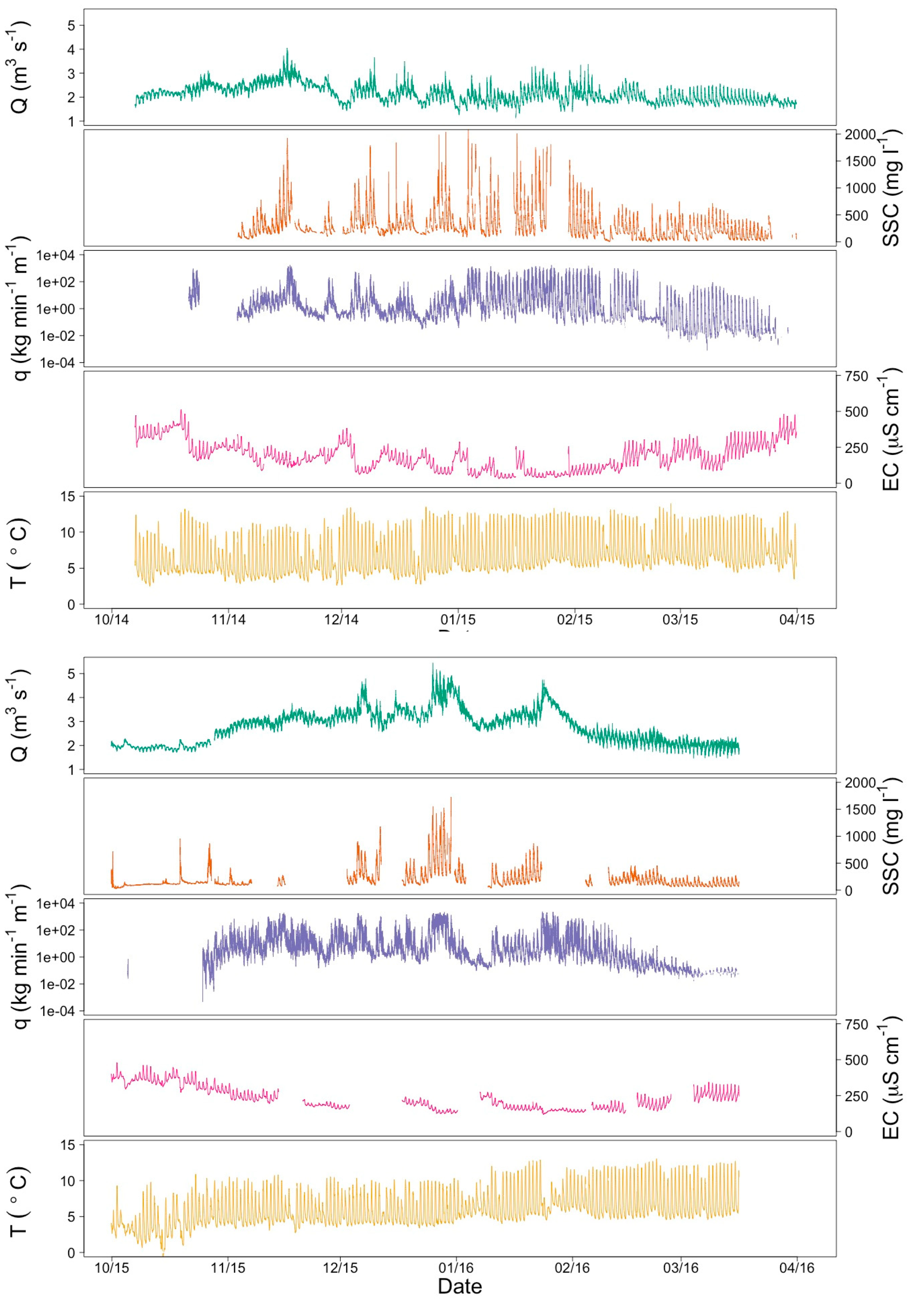
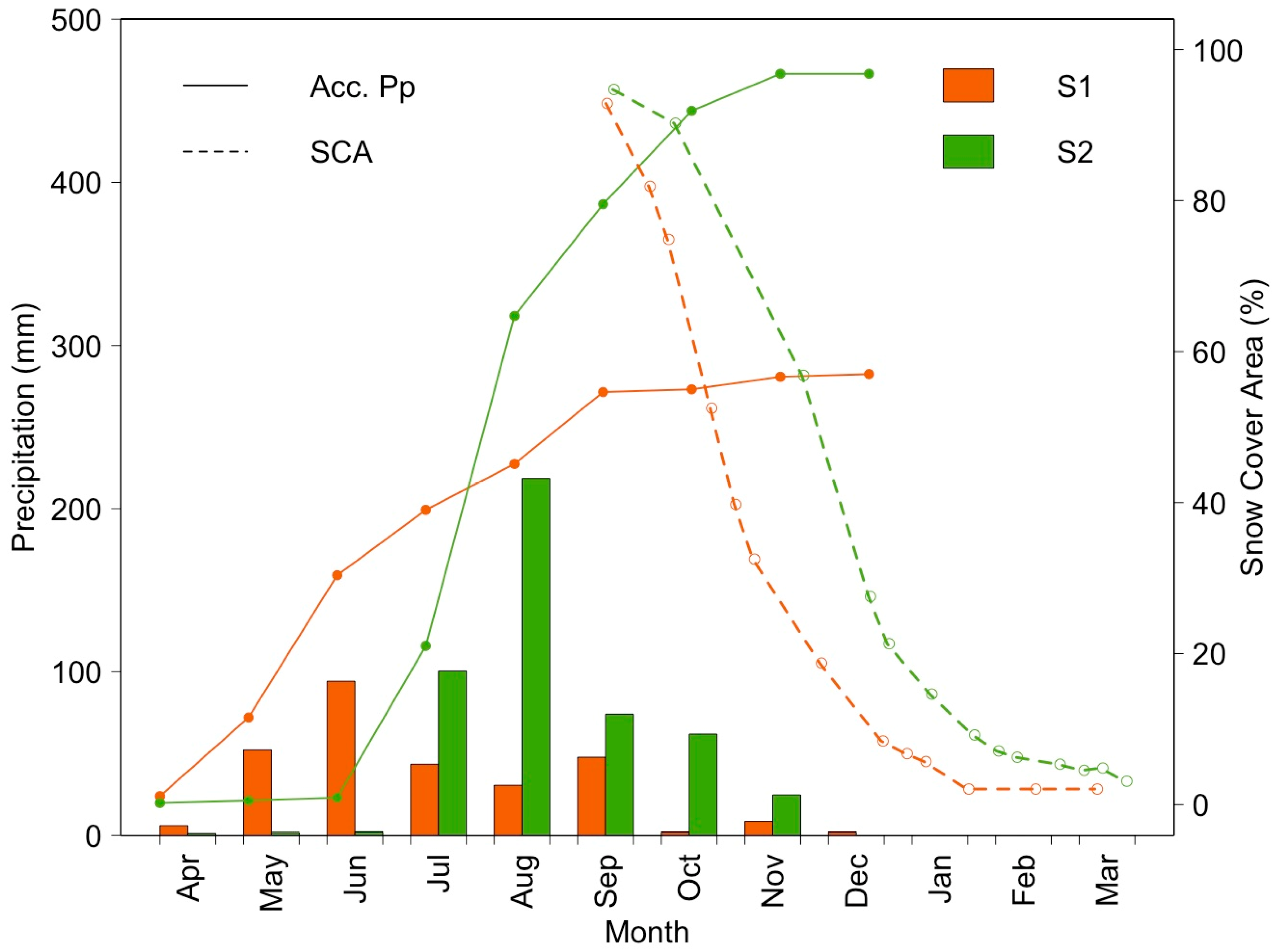
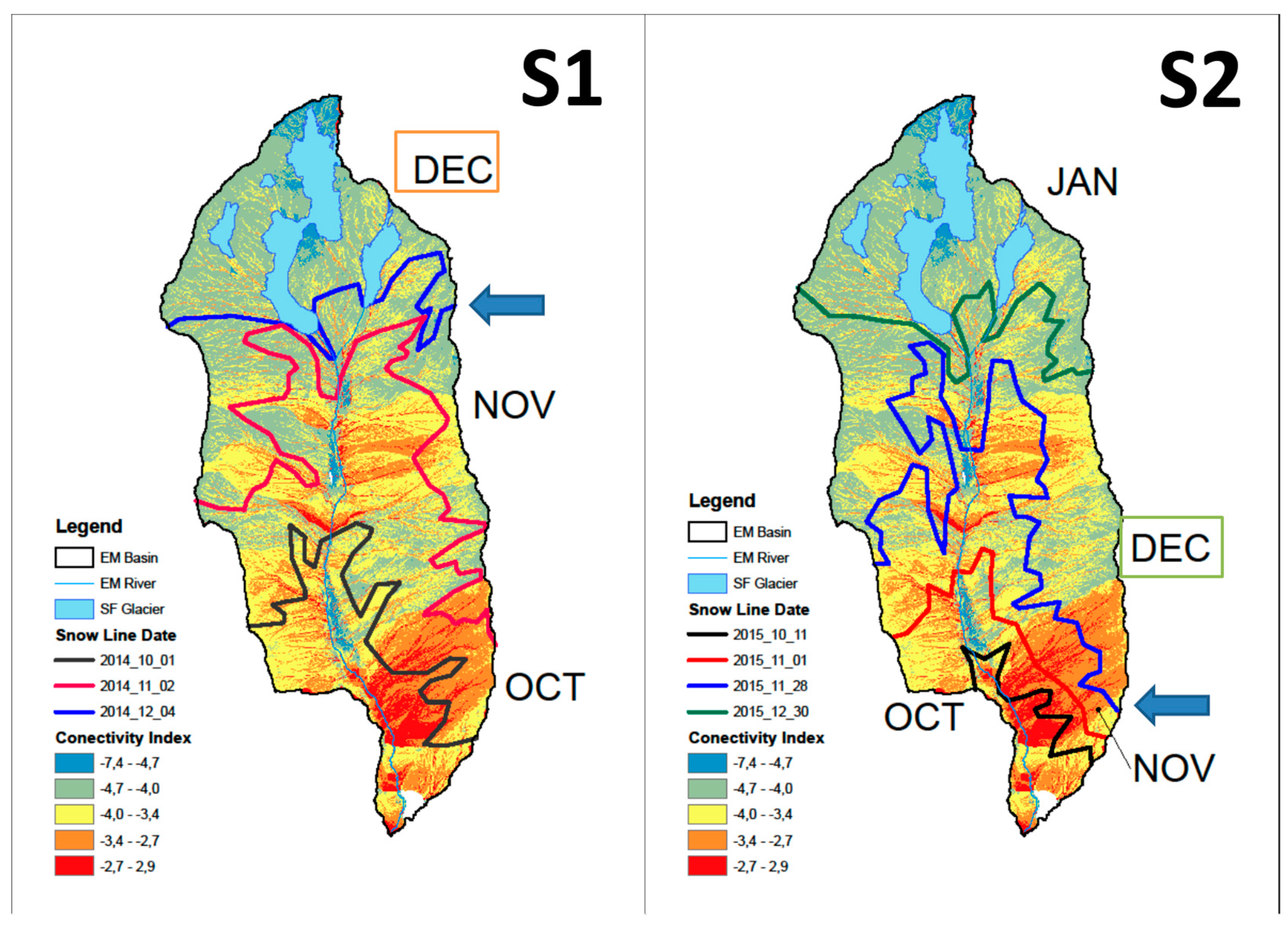
Snowmelt is arguably the main source of runoff in the period in which the percentage of snow cover area is reduced in the basin (
Figure 13), which is matched by the beginning of daily fluctuations of discharge (
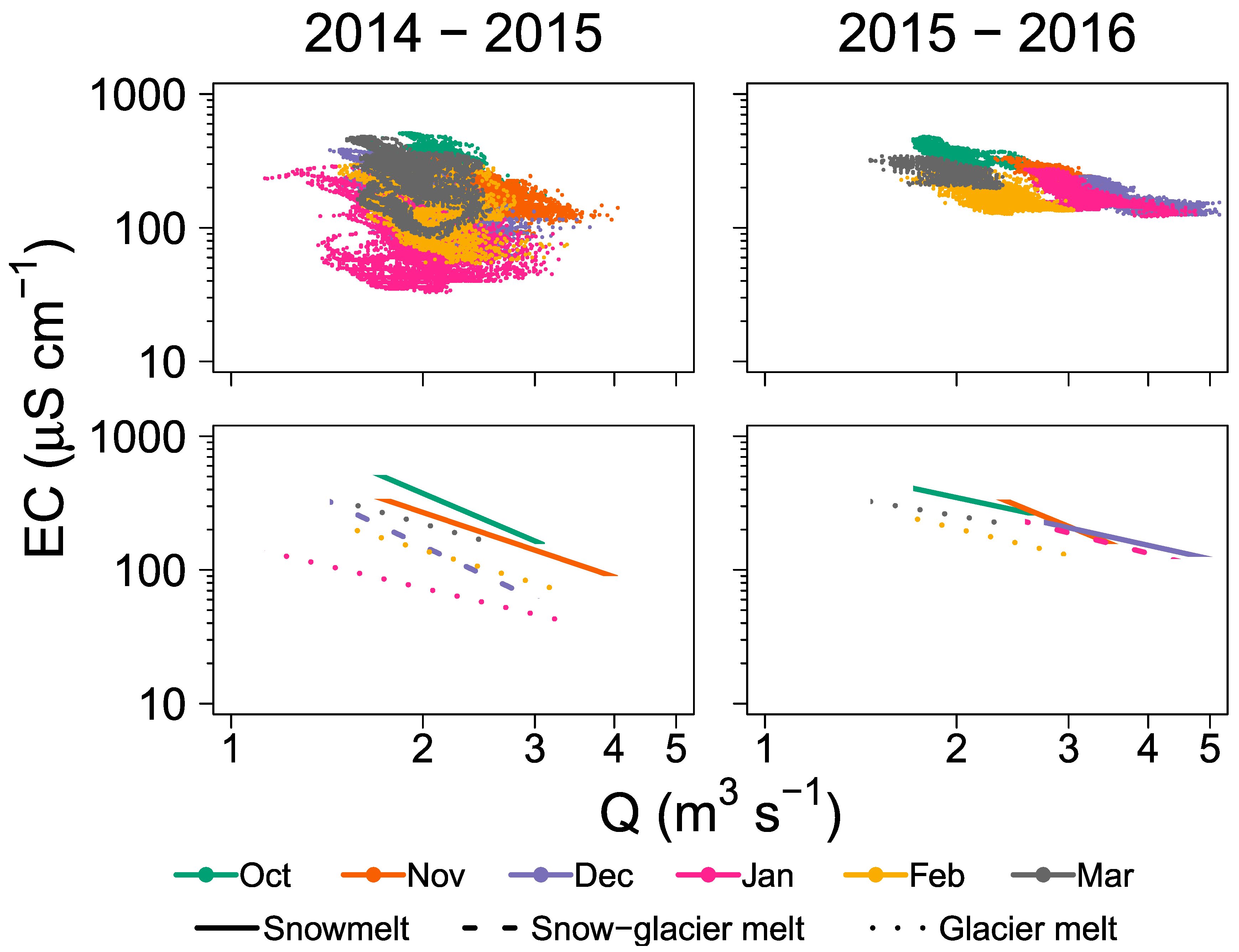
Figure 3). For the S1 and S2 ablation seasons, snowmelt dominates in October to November and October to December, respectively. The temporal variation on the relationship between Q–EC matched what was observed previously in other basins (e.g., [
14,
30]), with high EC at the snowmelt period and a continuous decrease of conductivity until the glacier melt period. In the Estero Morales, it is thus likely that January and February are characterized by pure glacier melting for the first and second year, respectively, given that the Q–EC regression lines plot the lowest (see
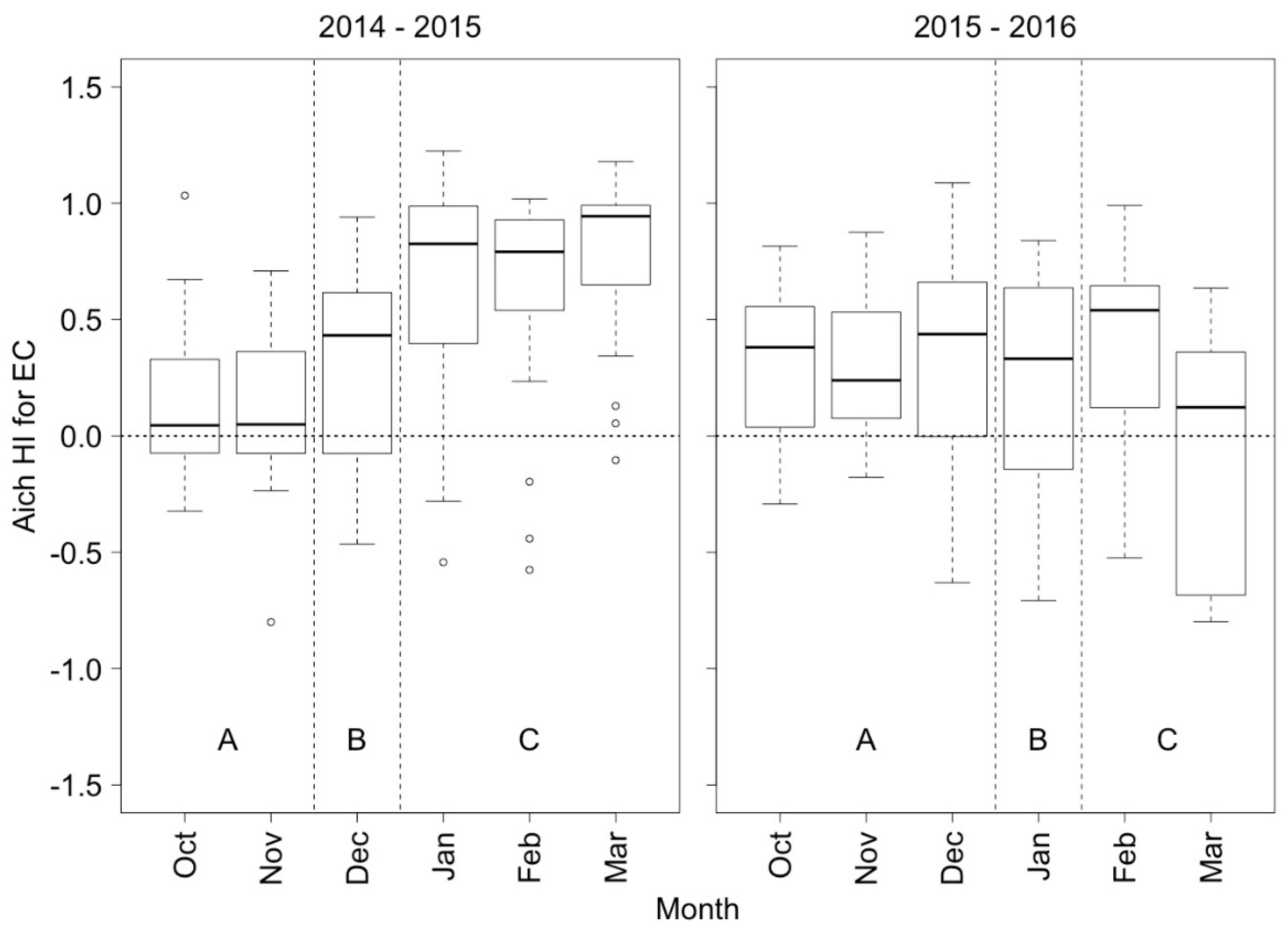
Figure 5) and the lack of snow cover in the basin. For the S1 ablation season, the hysteresis index for EC changes from a stronger to a weaker clockwise pattern, with an abrupt change in December (
Figure 6), which could be interpreted as the transition from the snowmelt (October and November) to glacier melt period (since January). Similarly, Collins [
31] found clockwise hysteresis during a glacier melt period due to the dilution of low-mineral glacier meltwater.
Differences in snow accumulation during winter and snow permanency in spring clearly affect the runoff, snowmelt infiltration, and groundwater contribution to streamflow. Limited snow accumulation (as for S1) leads to higher infiltration than runoff, and this is likely reflected in a weaker hysteresis between Q and EC. On the other hand, higher snow accumulation (as for S2) caused a relatively higher contribution to direct runoff rather than snowmelt infiltration, and also a larger hysteresis loop pattern due to a higher contribution of diluted water from snowmelt than mineral-enriched groundwater during falling limbs of daily hydrographs.
When snow cover becomes negligible, glacier melting becomes the dominant source of runoff in the Estero Morales. This transition happens in January and February for the S1 and S2 ablation seasons, respectively, when the Q–EC relationship begins to increase. This was also reported by Richards and Moore [
14] for the autumn recession limb in the Place Creek basin (Canada), due to the increase of groundwater contribution. Hysteresis features a clockwise trend from early glacier melt to the end of the glacier melting season for the first year, suggesting that glacier melt continued contributing meltwater to the system, diluting the small groundwater contribution during the falling limb of the daily hydrographs. On the other hand, the shorter glacier melt period due to higher snow accumulation in the second year, triggered higher rates of infiltrated snowmelt water during the entire ablation season. This could have affected the recession limbs in March, causing both clockwise and counterclockwise hysteresis, due to poor dilution of glacier meltwater on the falling limb during some days (clockwise) and high groundwater contribution on the falling limb (counterclockwise) on other days. Additionally, change in water storage on the hydrological glacier system affects the hydrochemistry of the water, where snow differences lead to differences in the glacier hydrological system and could also be responsible for the difference between ablation years.
4.2. Dynamics of Suspended Sediment Transport
In the Estero Morales, the SS transport dynamics was analyzed by using the Q–SSC relationship, SS yield, and the trends of hysteresis index, showing strong dependency to the melting seasons. The Q–SSC and HI are used to infer sediment availability and sources, due to differences in SSC for a given Q depending for each month and during a single flood (hysteresis, rising and falling limb; [
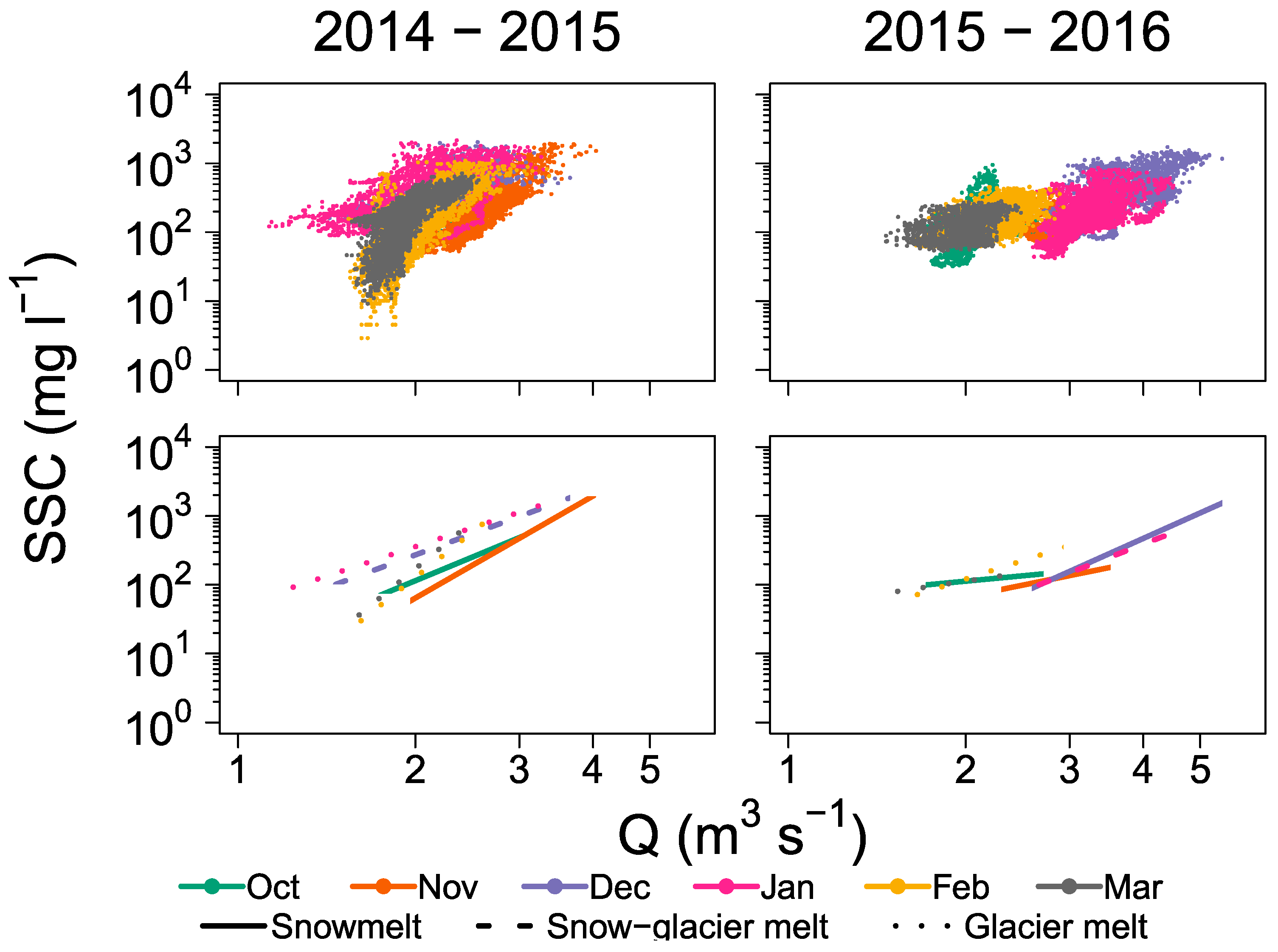
2]). During the first ablation year, the origin of runoff relates well with the Q–SSC relationship (
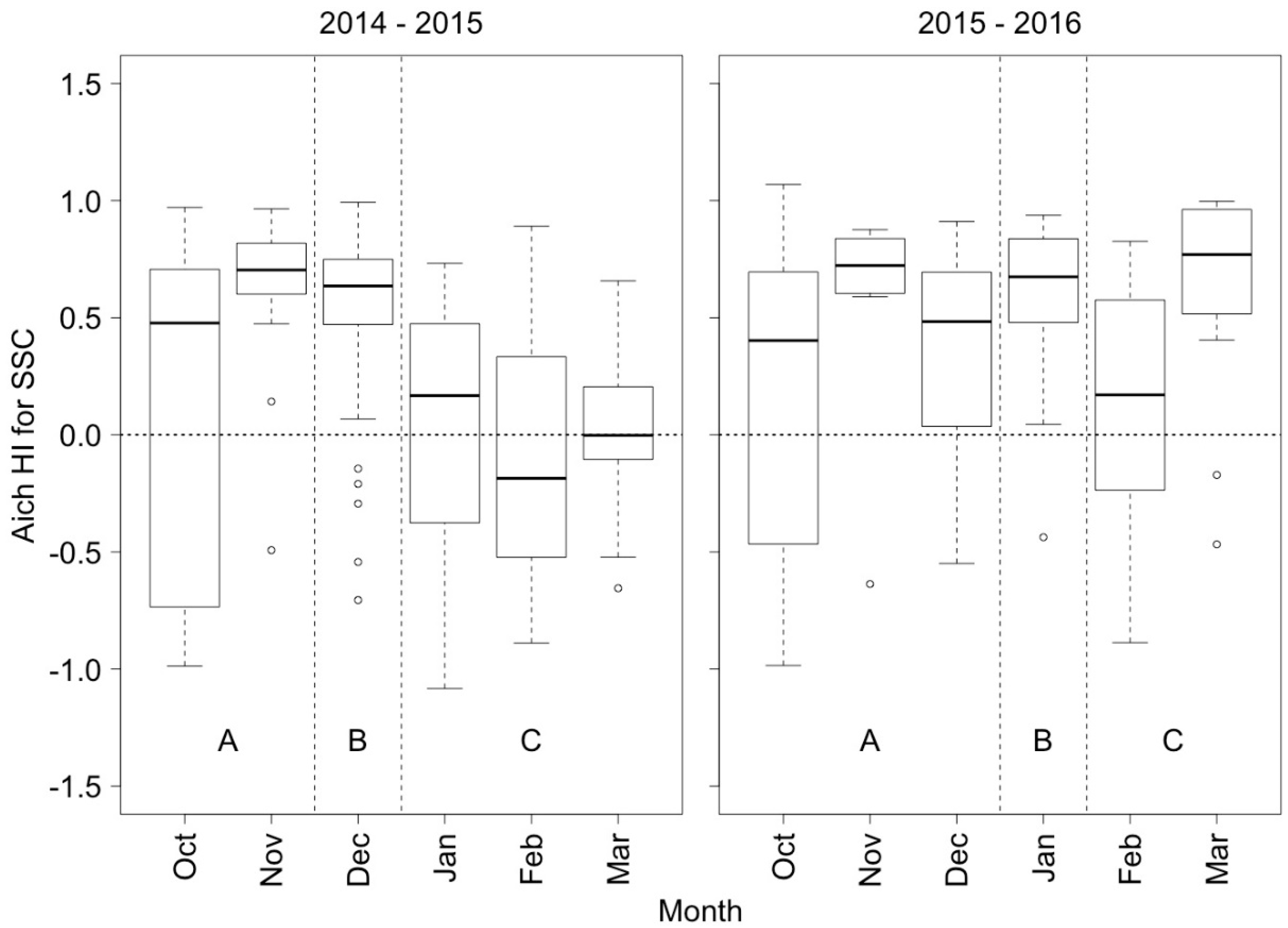
Figure 7). During snowmelt, fine sediments are likely not available in large quantities and are transported in low concentration at a given discharge. Despite the low availability of fine sediments during snowmelt, the HI index reveals a marked clockwise hysteresis (
Figure 8; S1). This is probably due to the proximity of sediment sources to the monitoring station (sediment sources during snowmelt being closer to the outlet of the basin if compared to the glacier melting period), fine sediment stored in the channel during previous ablation season [
14], bank failure, and slope wash by the runoff from melted snow [
32], creating readily available fine sediments for transport, especially during the rising limb of hydrographs [
2]. Sediment availability then appears to increase in the snow–glacier melt mix period (December), as fine sediments stored in great amounts in the proglacial area begin to be connected to the network by the origin of snowmelt runoff in the upper part of the basin. The hysteresis remains clockwise, supporting the interpretation of the presence of abundant and readily available fine sediments in the proglacier area [
19,
33]. Suspended sediment yield during snowmelt and snow–glacier melting transition were rather low, meaning that hillslopes and the proglacier area were only partially coupled to the channel, yielding a low quantity of sediment to the outlet. Later in the season, glacier melt reaches the maximum sediment availability of the season, but it is progressively decreasing towards the end of the season, suggesting a depletion of fine sediment coming from the glacier area. Likewise, hysteresis progressively shifts from clockwise to counterclockwise, supporting the interpretation of a progressive depletion of sediment sources in the glacierized area from early glacier melt to the end of the ablation season [
2,
20,
34]. Furthermore, the difference in the SSC peak during glacier melt could be interpreted as a change in sediment sources under or over the glacier, from the snout of the glacier in early glacier melt to the upper part of the glacier in late glacier melt. The dynamics of sediment connectivity due to glacier movements can be complex, and the reworking of sediments in the paraglacial area can indeed alter the local lateral and vertical connectivity (e.g., [
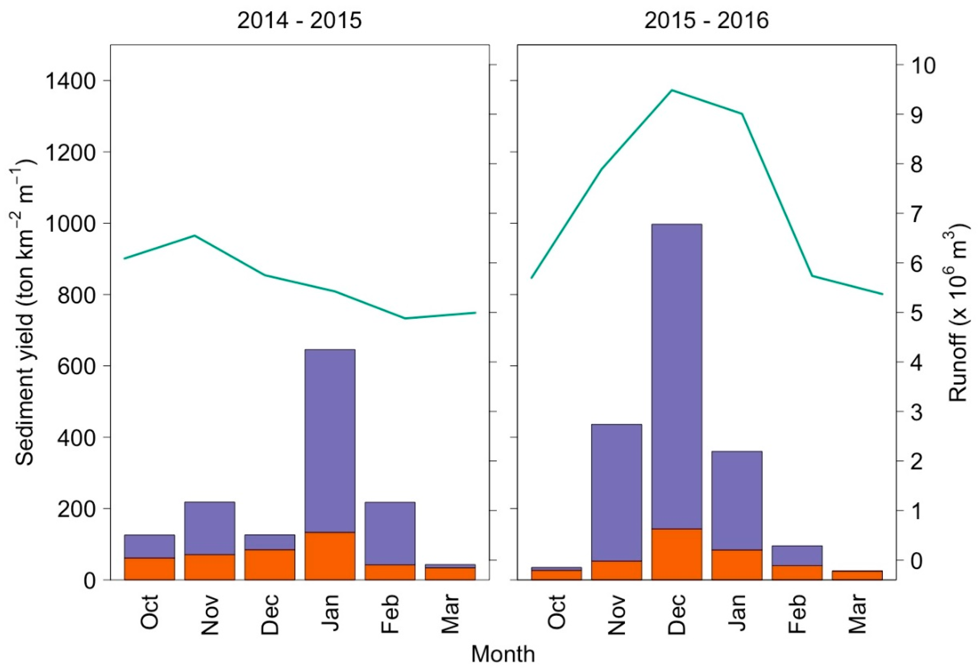
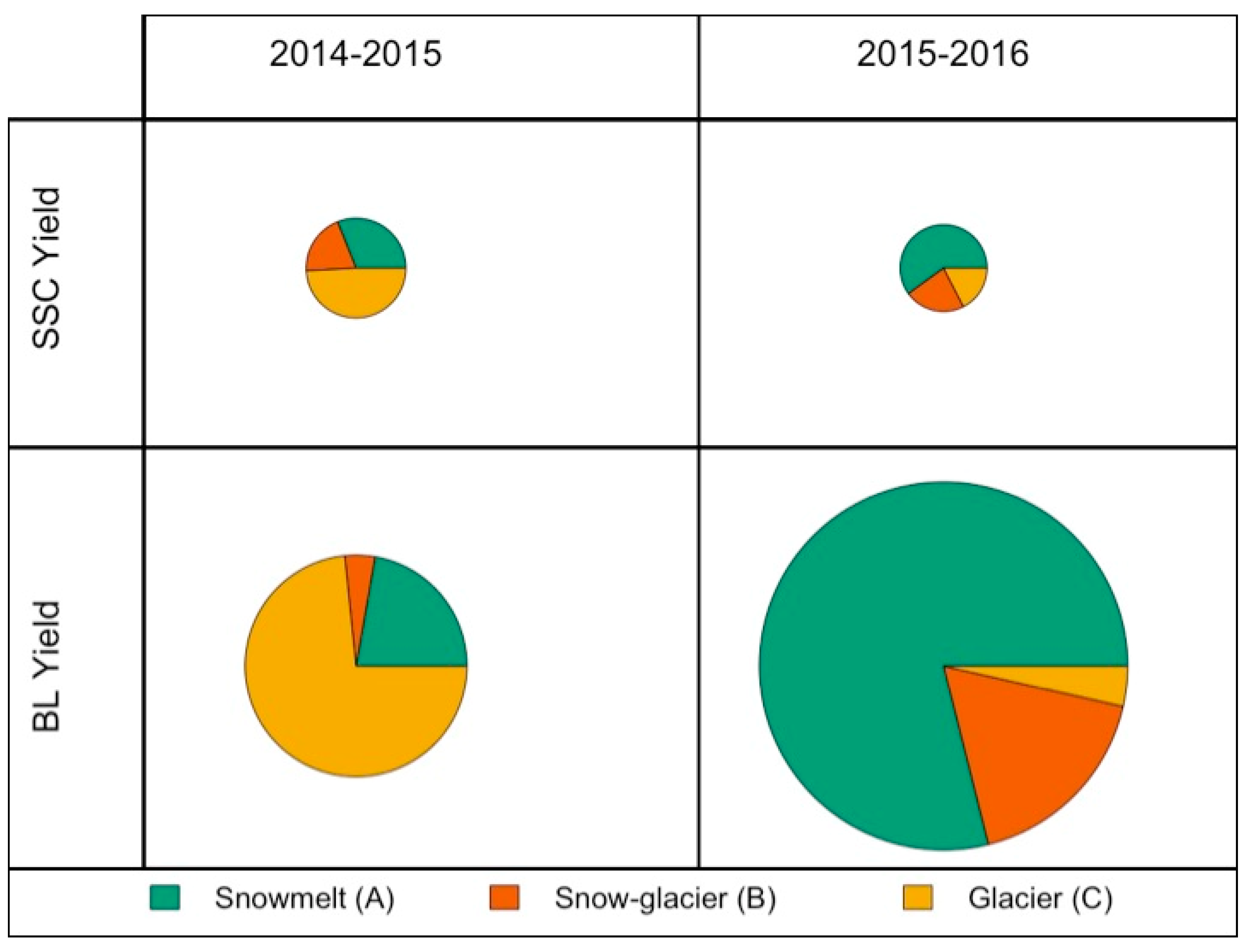
35]), changing sediment transport dynamics in the downstream river. Sediment yield also reaches the maximum during the early glacier melt period, coinciding with the high availability of SS in January. Additionally, half of the total SS yield of the S1 ablation season was produced by the glacier melt period (
Figure 14), highlighting the importance of the proglacial area in the SS production. At the end of the season, SS availability and yield decrease towards zero as the runoff reaches the baseflow and daily fluctuations of discharge become negligible. Interestingly, despite the very small transport of sediments, the HI shifts from counterclockwise to no hysteresis, suggesting a final change of the main source of sediments, from the proglacial area to remains of fine sediments stored in the lower portion of the main channel.
For the second year of observation, the Q–SSC relationship shows no trend in availability during the ablation season (
Figure 7). Overall, for the S2 ablation season, SSC appears to be more related to water discharge than water sources, showing less seasonal dependence than the year before. From the beginning of the season to the end of the snowmelt period, SS yield constantly increases (
Figure 7), probably due to the increase in water discharge caused by the increase in temperature. Indeed, sediment yielded by snowmelt represents more than half of the total transport for the year (
Figure 14). The HI shows clockwise hysteresis for the snowmelt period, but the small decrease in the HI from November to October reveals the change in fine sediment sources from closer sources to a farther sources [
19], driven by change in snow cover areas on the basin. However, this HI pattern could also suggest readily available sediments from slopes and channel sources [
2]. During the snow–glacier melt transition, fine sediments collected from the proglacier area are produced and transported downstream, yielding almost a quarter of the total SS for this season (
Figure 14). The HI reveals the high availability of fine sediments, as the hysteresis pattern is markedly clockwise. Finally, the pure glacier melt period in February and late glacier melt period in March represent the lowest SSC and yield for the ablation seasons (
Figure 12). Sediments coming from the glacier represent only less than a quarter of the total sediment yield (
Figure 14). Additionally, sediments are likely provided only from the glacier snout or the lowest part of it, due to the clockwise hysteresis in February (
Figure 8) and the lack of counterclockwise hysteresis that reveals activation of distant sediment sources. As in the previous year, late glacier melt is able to transport sediment stored in the main channel (near the measuring section, no hysteresis) but in small quantities (low yield;
Figure 12).
4.3. Dynamics of Bedload Transport
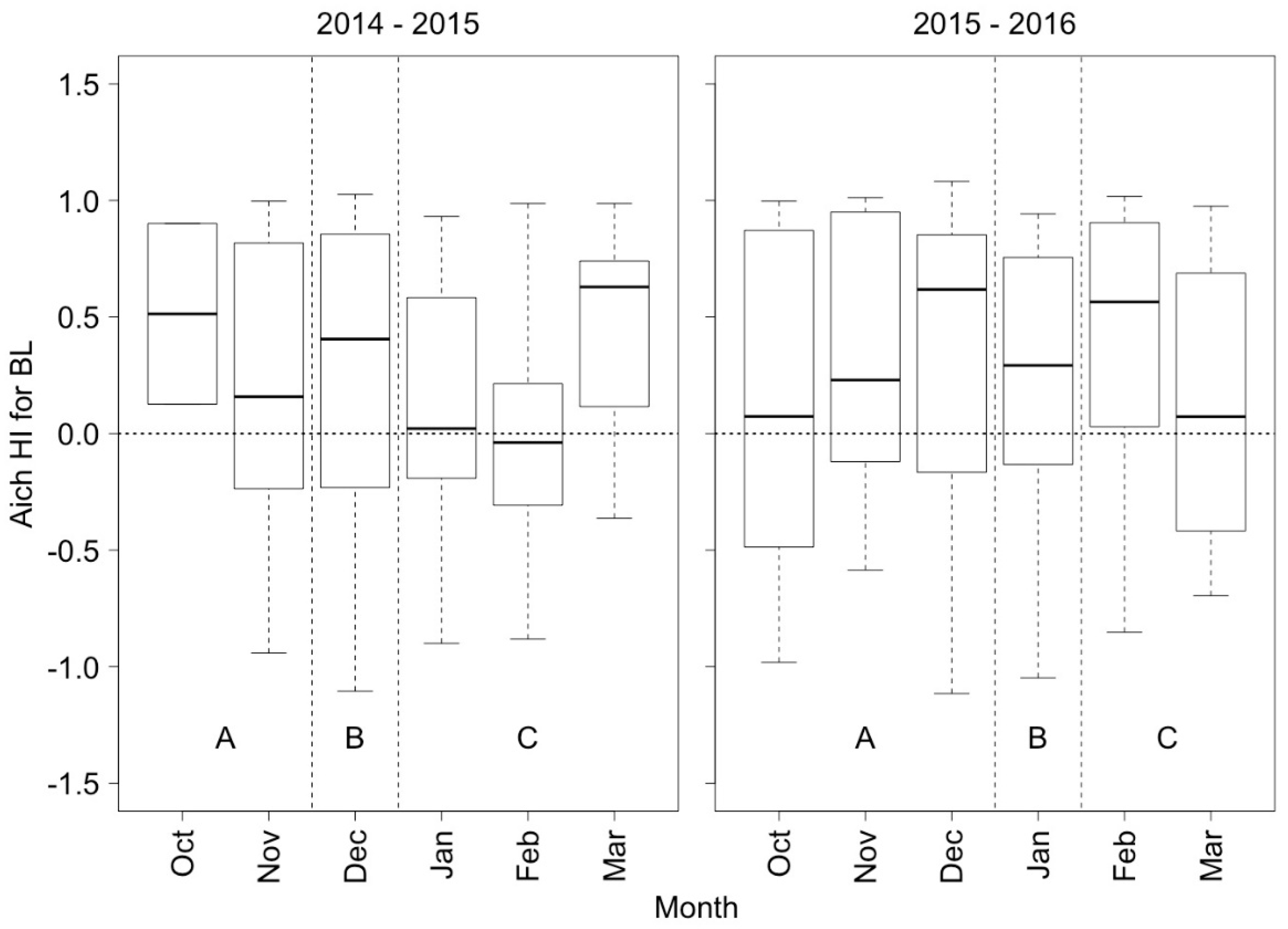
As for suspended sediment transport, bedload yield and availability are clearly dependent on the origin of runoff. In the first ablation season (2014–2015) the Q–BL relationship shows how the early glacier melt period features higher sediment availability than the snowmelt period. Furthermore, BL yield is also higher during glacier melt, representing almost three quarters of the total BL yield of the season (
Figure 9). Bedload efficiency also reaches its maximum during the early glacier melt period, decreasing to the end of the ablation season. Furthermore, hysteresis index reveals that coarse sediments are mainly provided from the proglacial area rather than other sources, due the constant decrease from clockwise to counterclockwise hysteresis, from snow–glacier transition to glacier melt, respectively (as in [
23]). As for the SS hysteresis, this change implies a likely change in the location of the main sediment sources, from the proglacier area to the glacier snout and finally more distant sources beneath the glacier. This highlights the crucial importance of the proglacial areas in supplying sediments to the system. By analyzing the morphological changes in the Haut Glacier d’Arolla (Switzerland), Perolo et al. [
36] revealed that the hydraulic efficiency of subglacial channels improves through the melting season, likely affecting bedload production due to phases of sediment clogging and flushing from subglacial channels to the downstream river. For the San Francisco Glacier, we cannot speculate on the existence or degree of importance of this process, and a more focused investigation on the temporal trend of glacier uplift and sediment transport dynamics immediately downstream could shed further light on the existence of such a process.
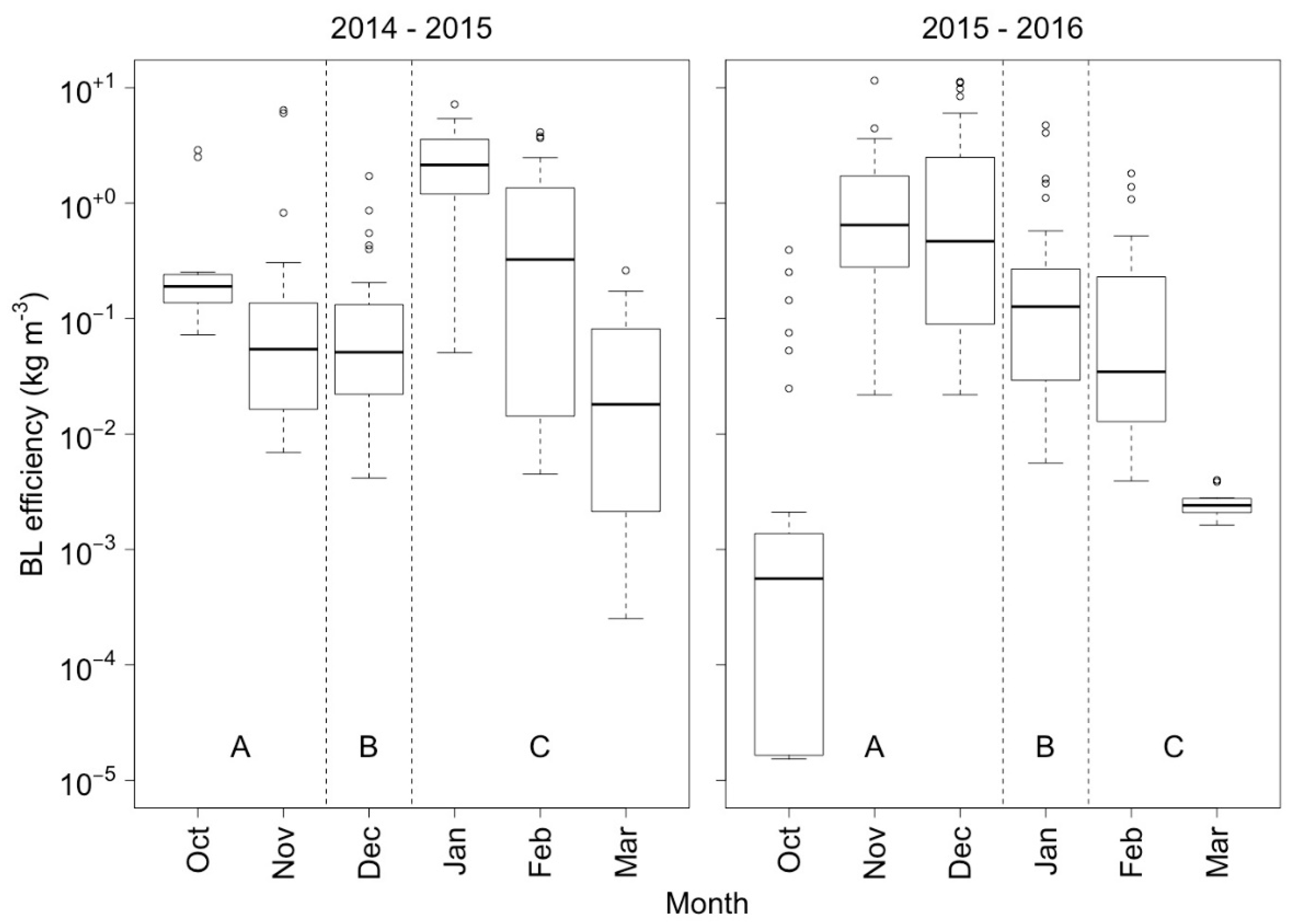
If compared with the snowmelt season, sediment availability (
Figure 9) and also sediment yield (
Figure 12) are lower, yielding low bedload transport efficiency during this period (
Figure 11). However, October features an average efficiency and high availability, but a rather low yield. Indeed, hysteresis reveals a high-magnitude clockwise pattern, which can be interpreted as that the sediment source is closer to the station, for instance, due to the breakout of the armor layer on the early snowmelt period and sediment supplied by highly connected slopes. Coarse sediment transport dynamics during the second ablation season were also determined by water sources. Snowmelt shows higher sediment availability (
Figure 9) and yield (
Figure 14), and bedload efficiency also remains higher for almost all the season (
Figure 11). The early snowmelt period contributes only partially to the annual bedload yield due to the late initiation of snowmelt on the ablation season, with very low bedload efficiency (
Figure 11). Further during the ablation season, snowmelt appears to couple the slopes throughout small tributaries, in addition to the release of sediments stored in the channel and from bank failures due to high water discharge [
11]. This process is also revealed by the nonhysteresis or low-magnitude clockwise patterns in November (middle snowmelt period), likely due to the wetness and saturated banks in high stage and the failure during and afterward [
32]. The ready availability of coarse sediments is inferred from the clockwise hysteresis in the final stage of snowmelt, probably due to the coupling of the slopes in highly connected places within the basin. This stage in the ablation season is critical, due the high availability and yield, supporting the idea that multiple sediment sources are well-coupled to the channel network due high spatial contribution of snowmelt and high water discharge. This complete snowmelt period contributes to more than three quarters of the total bedload yield on this ablation season. Snow–glacier melt transition presents the lowest sediment availability of the season and lower sediment yield and efficiency than during the snowmelt period. At the same time, the HI decreases, suggesting the dominance of farther sediment sources as main sediment suppliers, which are mainly in the proglacial area [
23]. During the first month of the glacier melt period, coarse sediment availability increases, sediments are transported at the same rate then as in the snow–glacier transition with less water discharge, and bedload efficiency partially decrease, but sediment yield is very low. At the same time, the HI is distinctly clockwise, hinting at the activation of sediment sources located near the glacier. This suggests that sediment sources near the glacier, which increase and have a completely different behavior compared to the rest of the season. However, and despite the high availability and activation of this source, water discharge is not effective at transporting large amounts of coarse sediments, making the early glacier melt a low-yield season, yielding only less than one quarter of the total yield. Finally, the quantity yielded by late glacier melt is negligible, with no variation on sediment rate with an increase of water discharge (
Figure 14).
4.4. Sediment Transport Dynamics on Both Ablation Seasons, and the Role of Coupled Sediment Sources
The interannual variability of sediment yield during the S1 and S2 ablation seasons can be related with differences in coupling mechanism on the sediment cascade, due to progressive changes for the type and location of the main sources of runoff and sediments in this glacierized basin. In terms of snowmelt, the most important difference between the ablation seasons is the timing of melting, which is retarded by a month in the second year (
Figure 13). Sediment dynamics during the snow ablation season is likely influenced by the depth of the snowpack and timing of the snow cover area on the basin. Indeed, snow avalanches could occur with high frequency and magnitude [
37], representing an important process of sediment displacement and a coupling factor between hillslopes and the main channel. Several studies (e.g., [
11,
12,
38]) demonstrated that snow depth directly influence the sediment transported by the avalanche. Sediments detached from the hillslopes and transported by avalanches in the main channel of the Estero Morales are likely to be higher in the second ablation season, as more snow accumulated over the winter (
Figure 13). Sediments transported by avalanches are finally coupled to the channel and released when the snow is melting and disappearing over it. Indeed, the highest sediment transport on S2 occurred during November and December (
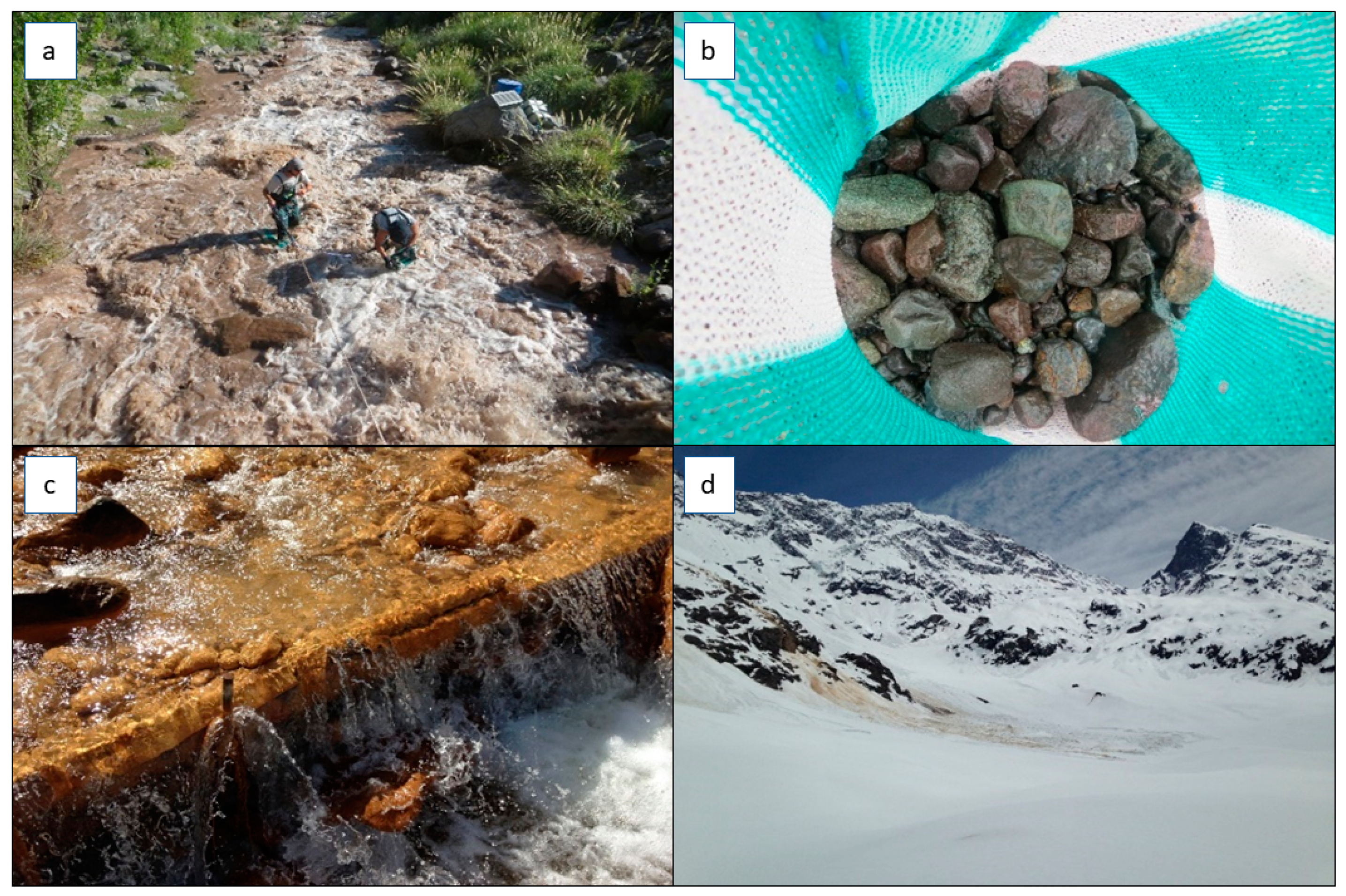
Figure 12), when sediments could be released from avalanche cones in highly connected zones over the channel, as shown in
Figure 2 for November and December. This process coupled the slopes on the S2, a process that does not appear to have happened in the previous ablation season, when snow accumulation was low and mainly in the early winter, and avalanches were probably less important in transporting sediments to the main channel. Indeed, sediment yield on the snowmelt season was substantially smaller than the second year.
Apart from the role of avalanches, the higher amount of snow in the second year and the later melting affected sediment yield. Higher water infiltration at the basin scale increases soil wetness [
39], thus making channel banks more saturated and more likely to collapse, supplying sediment to the system [
32]. The occurrence of this process is also suggested by Iida [
32], who related bank collapse to counterclockwise hysteresis—almost the same pattern observed in November of the second year in the Estero Morales, but for bedload transport. Despite SS yield leading by snowmelt was higher in the second year, comparing October and November between years, higher values were found during the first year. This was due to the higher snowmelt rate that was present during those months for the first year than the second, represented by the slope of snow cover area in
Figure 13, while December was the higher slope for the second year. Proglacial areas have been recognized as an important source of sediments [
35,
40]. Despite the high quantity of unconsolidated material in this zone, the BL export in the Estero Morales changed from one year to another. Higher snow accumulation probably leads to higher likelihood of avalanches and more runoff that mobilizes sediments to the network, as occurred during the second ablation season. When the snow accumulation is lower, as in the first year in the Estero Morale, snow is less effective as a coupling factor for the proglacier area, leading to a lower sediment yield. In contrast, SS yield was similar for both years, suggesting that the proglacier area is a source of unlimited supply of fine sediment. The high-magnitude clockwise hysteresis seems to support this interpretation, suggesting readily available sediments during this period.
4.5. Insights on Likely Future Trends of Sediment Transport Dynamics on the Estero Morales
Protected as a natural reserve and lacking major anthropogenic influences (apart from limited horse grazing in summer), the Estero Morales basin is an important site to study changes in climate and the response in terms of glacier dynamics and associated geomorphological processes, including sediment transport. Due to the generalized increase of temperature and increase of elevation of the 0 °C isotherm in the region, associated as well with reduced precipitation and “extremization” of rainfall events, the San Francisco Glacier experienced a retreat over the past years [
41]. The nearby El Morado Glacier, which is located in a basin immediately to the west of the study basin, experienced an areal loss of 40% between 1955 and 2019, with an increased retreat and thinning during the last decade, which coincided with a severe drought in the region [
42]. The Estero Morales and the numerous other glacierized Andean basins in the region will thus suffer unpredictable changes in terms of sediment yield and dynamics due to a general lack of knowledge and understanding on the long-term effects of glacier recession on sediment production and legacy in terms of river morphological evolution [
43]. In its recent contribution, the IPCC report on high mountain areas [
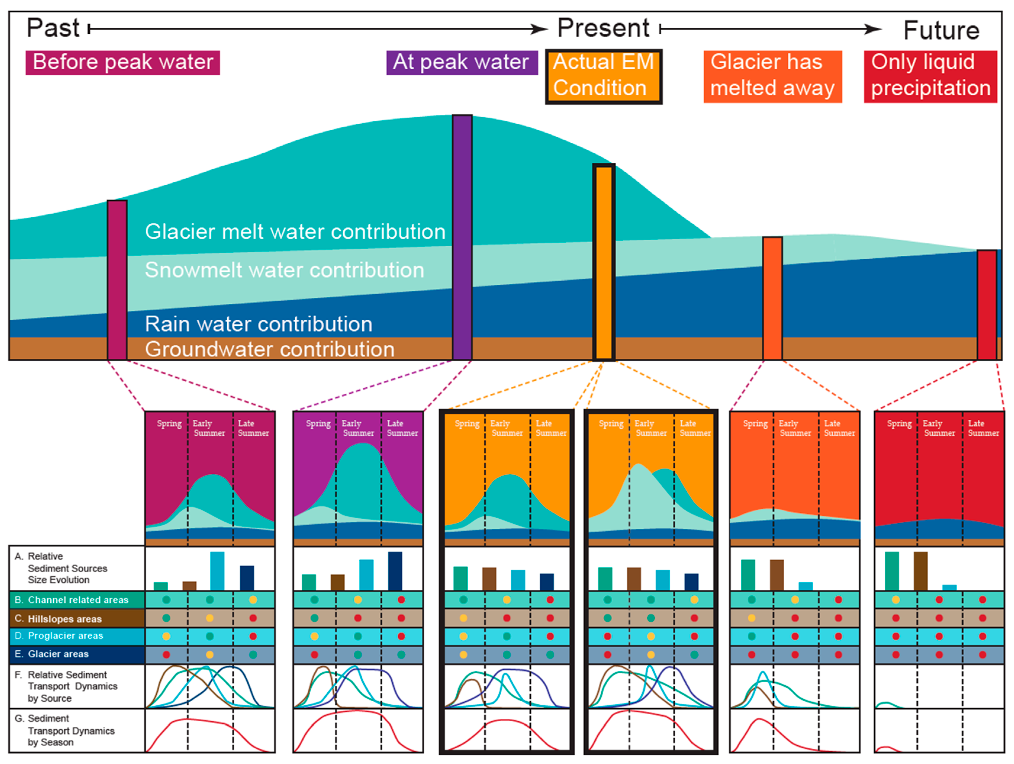
44] presented a conceptual model on the water discharge contribution between glacier, snow, and rain that occurs in a glacierized and changing basin at different temporal scales.
Figure 15 is based on that conceptual figure and extends to longer term periods. We included in the conceptual figure the sediment transport dynamics component and associated factors according to the water contribution for each stage at seasonal scale. This includes the relative importance of sediment sources (in-channel, hillslopes, proglacial, and glacial), the elative sediment transport dynamics by sources for each ablation condition, and the sediment transport dynamic by season. Stage (i) is typically characterized by a constant increase of water discharge because of increased glacier melting, due to the increase of air temperature and a decreasing snow-to-rain ratio. At peak water discharge (stage (ii)), the glacier is large enough to melt the maximum water discharge coming from ice melting in the history of the glacier, due to the constant increase in temperature. After the peak discharge, due to the decreasing glacier volume and despite the increase in temperature, water melted from the glacier starts to decrease until the glacier is melted away (stage (iv)). The total water discharge decreases and is totally due to rainstorms and a progressively reduced amount of snowfall.
In its actual conditions (stage iii), the Estero Morales basin is possibly between stages ii and iv, where water discharge is decreasing due the shrinking San Francisco Glacier, and the peak of water discharge leading by glacier melting is already reducing. The lack of long-term monitoring of discharge makes it difficult to demonstrate, but the qualitative testimonials of locals and park guards would suggest it. A regional study on the regional glacier retreat over the last 100 years shows a rapid decrease rate on frontal variation of the glaciers, with a more recent reduced rate [
42,
45], which suggests that the peak discharge of those basins might have been reached during the maximum ice retreat around 1980, approximately. Dussaillant et al. [
46] analyzed the water discharge variations and the contributions from the glaciers in the last 18 years on the Maipo basin in El Manzano (a gauging station in the Maipo basin). They found a reduction of 32% in the annual mean river runoff by comparing 2000–2009 and 2009–2018 study periods, suggesting that glaciers within the basin, including the San Francisco Glacier, are probably between stages ii and iv. Likewise, the snow cover extent for each winter season in the entire region has been decreasing in recent years, as demonstrated by Malmros et al. [
47] for the years 2000–2016. This is also supported by the fact that the elevation on the 0 °C isotherm in the region has increased around 150 m between 1975 and 2001 [
48]. All of these regional observations support the belief that the Estero Morales is already experiencing a decrease of water discharge provided by the glacier, and it is likely that the melted ice supply to the total discharge will be decreasing continuously until the glacier is entirely melted.
Figure 15 provides a conceptual interpretation of the past and future changes in terms of hydrological functioning and sediment yield in the Estero Morales.
Stage i: When the San Francisco Glacier extended farther into the basin in the past (similar to the nearby El Morado Glacier; Farias-Barahona et al. (2020)), the water discharge was likely dominated by a mix of snowmelt and glacier melt, and the main source of sediment was the small proglacial area progressively left exposed by the retreat of the glacier. Despite the glacier covering a large part of the basin, most of the subglacier sources were inactive, due to low temperatures, leading to short ablation seasons. The small proglacial areas sourcing sediments were well-coupled in spring and summer, whereas subglacier sources would start to be coupled from midsummer until the end of the season. Furthermore, the glacier was not coupled at the beginning of the season to the high snow accumulation on the glacier surface and the surroundings.
Stage ii: At this stage, water runoff was dominated by glacier melt rather than snowmelt due to the increase in temperature, despite that the glacier was smaller than at stage i. In this stage, the sediment source from the glacier itself became more relevant because the ablation season started earlier than during stage i, due to the reduction in snow accumulation and the increase of air temperature. This made the subglacial hydrology more developed and able to reach more extended sediment sources under the glacier. Hillslopes and channel became larger sources of sediments because these were uncovered by the glacier and snow accumulation, and sufficient to couple this sediment source in spring, but the coupling likely decreased throughout the season. On the other hand, the proglacial area was higher in altitude so it became completely coupled at the beginning of the summer and uncoupled when the snow melted away. Glacier sediment sources became active and sediments were transported downstream during the entire summer, starting before and longer than during stage i. At the end of the season, only glacier sources were coupled to the channel network.
Stage iii: In the present conditions, the Estero Morales could face winters with high or low (and early or late) accumulation of snow in winter. This leads to different conditions for coupling of sediment sources and sediment yield, reflected by the evidence presented and discussed in the previous sections.
Stage iv: In a condition in which the glacier disappears completely due to reduced replenishment (high temperature, limited snowfall in winter), the snowmelt and rainfall will be the only components of runoff (apart from the groundwater contribution). The sources of sediments in the proglacial sediment area will be activated only by rainfall and snowmelt. Because the coupling of channel and hillslope sources will be modulated by snow processes, the high reduction of snow accumulation will lead to only midcoupling of hillslope, channel, and proglacier sources, and concentrated only in spring. Summer periods will be characterized by low discharge and sediment transport, supplied by channel processes until midsummer, leading to an end of the summer with no important sediment transport, albeit during late autumn intense rainfall events.
Stage v: In this scenario, the rise of the isotherm would reduce the snowfall to zero. This will leave the same sediment source areas as in stage iv, but with less or no proglacier area. Under these circumstances, it is possible to imagine a denser cover of vegetation at the basin scale, too, which will reduce even more the delivery of sediments to the hydrological network. Sediment sources will be represented only by channel processes (and sediment sources well-connected to the network), with only groundwater runoff and some summer storms.


